


Preface
The following set of papers describe in detail the science goals of the future Space Infrared telescope for Cosmology and Astrophysics (SPICA). The SPICA satellite will employ a 2.5-m telescope, actively cooled to around 6 K, and a suite of mid- to far-IR spectrometers and photometric cameras, equipped with state of the art detectors. In particular, the SPICA Far Infrared Instrument (SAFARI) will be a grating spectrograph with low (R = 300) and medium (R ≃ 3000–11 000) resolution observing modes instantaneously covering the 35–230 μm wavelength range. The SPICA Mid-Infrared Instrument (SMI) will have three operating modes: a large field of view (12 arcmin × 10 arcmin) low-resolution 17–36 μm spectroscopic (R ~ 50–120) and photometric camera at 34 μm, a medium resolution (R ≃ 2000) grating spectrometer covering wavelengths of 18–36 μm and a high-resolution echelle module (R ≃ 28000) for the 12–18 μm domain. A large field of view (80 arcsec × 80 arcsec), three channel, (110, 220, and 350 μm) polarimetric camera will also be part of the instrument complement. These papers will focus on some of the major scientific questions that the SPICA mission aims to address, more details about the mission and instruments can be found in Roelfsema et al. (Reference Roelfsema2017).
1 Introduction
One of the biggest questions in current astrophysical research is how star formation and black hole accretion activities evolved throughout cosmic history. In order to answer the question, we need efficient methods to study the spectral properties of a large sample of galaxies in a systematic way, and thereby trace not only those activities over cosmic time, but also the profound relationship between the two phenomena through spectral diagnostics of the physical conditions of the interstellar/circumnuclear media in galaxies. It is particularly important to cover the peak phases of the two phenomena, which occur in the redshift range of z = 1–3 (Madau & Dickinson Reference Madau and Dickinson2014), and that redshift range corresponds to the cosmic time where dust extinction is most severe, making any UV, optical, and near-infrared (IR) observations prone to large systematic errors which render the results highly unreliable. X-rays are useful for detecting an active galactic nucleus (AGN), but can miss the population of Compton-thick AGN. The mid- to far-IR spectral range contains an enormous number of ionic, atomic, and molecular lines and dust features as spectral diagnostic tools (e.g., Spinoglio & Malkan Reference Spinoglio and Malkan1992). Hence, IR spectroscopic surveys from space are crucial.
More specifically, in the mid-IR range, there are many important spectral bands of dust particles and very large molecules such as silicates, carbonaceous grains, and ices. Among them, emission features due to polycyclic aromatic hydrocarbons (PAHs) are ubiquitously observed from photo-dissociation regions (PDRs), which are widely distributed around star-forming regions in a galaxy (e.g., Hollenbach & Tielens Reference Hollenbach and Tielens1999). The PAH emission is also detected from the diffuse interstellar medium. Their emission features are detected not only from many nearby galaxies (e.g., Smith et al. Reference Smith2007), but also from distant galaxies up to redshift z ~ 4 (Yan et al. Reference Yan2007; Sajina et al. Reference Sajina, Yan, Fadda, Dasyra and Huynh2012; Riechers et al. Reference Riechers2014; Kirkpatrick et al. Reference Kirkpatrick2015). PAHs are believed to be the most important heating agents of gas in PDRs (e.g., Weingartner & Draine Reference Weingartner and Draine2001), and thus their emissions are crucial probes to study the interstellar media associated with star-formation activity. In particular, PAH spectral features at 3.3, 6.2, 7.7, 8.6, 11.3, 12.7, and 17 μm, which are attributed to C–C stretching and C–H bending modes, are notably strong compared to fine-structure gas lines for star-forming galaxies, though PAH spectral features are relatively broad. Hence, they are powerful tools to determine the redshifts of faint distant galaxies, and can also trace star-formation activity since PAH features are characteristic of PDRs (e.g., Lutz et al. Reference Lutz2008; Teplitz et al. Reference Teplitz2007; Takagi et al. Reference Takagi2010; Bonato et al. Reference Bonato2015; Shipley et al. Reference Shipley, Papovich, Rieke, Brown and Moustakas2016).
The PAH features are also useful to estimate the relative contribution of an AGN and the star-formation component to the total IR luminosity L IR of a galaxy; the emission from PAHs is expected to be suppressed by photo-dissociation of PAHs due to the hard UV and X-ray radiation field from the AGN, while the mid-IR continuum emission is enhanced because of heating of circumnuclear dust by the same radiation (Oyabu et al. Reference Oyabu2011; Lacy et al. Reference Lacy2013). Therefore, the equivalent widths of the PAH features enable us to roughly estimate the star-formation contribution to the total L IR of a galaxy (Moorwood Reference Moorwood1986; Roche et al. Reference Roche, Aitken, Smith and Ward1991; Genzel et al. Reference Genzel1998; Armus et al. Reference Armus2007; Imanishi et al. Reference Imanishi2007, Reference Imanishi2008, Reference Imanishi, Nakagawa, Shirahata, Ohyama and Onaka2010; Veilleux et al. Reference Veilleux2009; Nardini et al. Reference Nardini2008, Reference Nardini2009, Reference Nardini, Risaliti, Watabe, Salvati and Sani2010; Pope et al. Reference Pope2008; Menéndez-Delmestre et al. Reference Menéndez-Delmestre2009; Coppin et al. Reference Coppin2010; Stierwalt et al. Reference Stierwalt2013, Reference Stierwalt2014), and more reliably estimate it when they are normalised with other spectral indicators (such as H2 or [Ne ii] 12.8 μm line fluxes) or the slope of the IR continuum (Tommasin et al. Reference Tommasin, Spinoglio, Malkan and Fazio2010). This approach is complementary to the one that uses spectral energy distribution (SED) fitting (e.g., Gruppioni et al. Reference Gruppioni2016; Delvecchio et al. Reference Delvecchio2014). Although the PAH features are bright and readily identified, it is also known that their interband ratios can vary from galaxy to galaxy to some extent, mainly depending on their ionisation states and/or size distributions which reflect the interstellar conditions (e.g., Allamandola, Tielens, & Barker Reference Allamandola, Tielens and Barker1989; Joblin et al. Reference Joblin, Hendecourt, Leger and Defourneau1994). Typical examples in the nearby universe are PAHs in early-type galaxies, where the PAH 6.2 and 7.7 μm features are significantly weaker than the PAH 11.3 μm feature (Kaneda, Onaka, & Sakon Reference Kaneda, Onaka and Sakon2005; Kaneda et al. Reference Kaneda2008; Panuzzo et al. Reference Panuzzo2011). The profiles of the PAH features, such as peak positions, widths, and relative strengths of plateau components, might also vary (e.g., Tielens Reference Tielens2008), providing us with information on the properties of the interstellar medium in a galaxy (e.g., aromatic/aliphatic ratios). In addition to the variations of the PAH features, complications from metallicity may be a serious issue, especially when we discuss galaxies at high redshift; the abundance of PAHs relative to dust is known to decrease significantly at low metallicities (Engelbracht et al. Reference Engelbracht2008).
The strong silicate features at 9.7 and 18 μm are often detected from a galaxy as either absorption or emission features. Similarly to the PAH features, the silicate bands provide us with information not only on the amount of silicate dust, but also on its properties such as size distributions, crystallinity, and the degree of processing (e.g., porosity, Fe/Mg, olivine/pyroxene; Henning Reference Henning2010; Xie, Li, & Hao Reference Xie, Li and Hao2017). In particular, the silicate features are the cornerstone of the AGN torus paradigm. Their profiles range from moderate emission, usually but not exclusively, in type 1 AGN, to deep absorption in the most dust-obscured AGN. The strength of the silicate feature is indicative of the optical depth of the hot dust heated by the active nucleus, and the relative strength between the features at 9.7 and 18 μm provides information on the distribution of the dust, as a smooth or clumpy medium (Hatziminaoglou et al. Reference Hatziminaoglou, Hernán-Caballero, Feltre and Piñol Ferrer2015). Furthermore, the combined information provided by the PAH and silicate features allows for an almost unbiased classification of objects into starburst- and AGN-dominated in the mid-IR (Spoon et al. Reference Spoon2007; Hernán-Caballero & Hatziminaoglou Reference Hernán-Caballero and Hatziminaoglou2011). Above all, both PAH and silicate features in the mid-IR are not mere tools to estimate star-formation rates and AGN contribution in a galaxy, but also important probes to study the physics governing the interstellar/circumnuclear media in a galaxy. The potential of those dust features as spectral diagnostics, however, is still not completely developed even in the nearby universe, much less at high redshift.
SPICA (SPace Infrared Telescope for Cosmology and Astrophysics), a 2.5-m large cryogenic telescope in space, will provide unprecedented high spectroscopic sensitivities with continuous wavelength coverage from the mid- to the far-IR (Roelfsema et al. Reference Roelfsema2017; Nakagawa et al. Reference Nakagawa2014). In particular, an extremely low-IR background achieved thanks to its primary mirror cooled down to below 8 K, is essential to study broad spectral features such as dust bands from faint objects. SMI (SPICA Mid-infrared Instrument; Kaneda et al. Reference Kaneda2016) is one of the two focal-plane scientific instruments planned for SPICA. SMI is the Japanese-led instrument proposed and managed by a university consortium, designed to provide a longer wavelength coverage and higher spectral mapping efficiency (i.e., higher spectral survey speed) compared to JWST (James Webb Space Telescope), in addition to high-resolution (HR) spectroscopic capability. In this paper, we focus on the scientific potential of unbiased large spectroscopic surveys with SMI. On the other hand, Gruppioni et al. (Reference Gruppioni2017) highlight the potential of large photometric surveys with SMI, they also describe the general scientific values of SPICA mid-IR survey datasets to reveal the evolution of the dust-obscured star-formation and AGN activity in galaxies since the re-ionisation epoch at z ~ 7. We plan to perform follow-up spectroscopy with the SPICA far-IR instrument, SAFARI, based on the results of the SMI surveys, which is essential to complete our IR spectroscopic studies of the evolutions of galaxies and materials therein.
Throughout this paper, we adopt the flat universe with the following cosmological parameters: Hubble constant, H 0 = 70kms−1Mpc−1, density parameter, ΩM = 0.3, and cosmological constant, ΩΛ = 0.7.
2 SPICA Mid-infrared Instrument (SMI) for large surveys
SMI has the following four channels in the mid-IR: spectroscopic functions for low-resolution (LR), mid-resolution (MR), and HR spectroscopy, and a photometric function for broad-band imaging (CAM). The main design driver for SMI/LR and /CAM is the ability to carry out large surveys, especially of PAH spectra (Wada et al. Reference Wada2017); a pioneering PAH spectral survey was performed by Bertincourt et al. (Reference Bertincourt2009) with Spitzer/IRS. SMI/LR is a multi-slit prism spectrometer system with a wide field-of-view covered by four long slits of 10 arcmin in length and 3.7 arcsec in width, thus enabling LR (R = 50–120) spectroscopic surveys with continuous coverage of the wavelength range of 17–36 μm. In the SMI/LR system, a 10 arcmin × 12 arcmin slit viewer camera (SMI/CAM) is implemented to accurately determine the positions of the slits on the sky for pointing reconstruction in creating spectral maps. SMI/CAM adopts an optical bandpass (30–37 μm) filter at a central wavelength of 34 μm and thus provides 34 μm broad-band images with a field of view of 10 arcmin × 12 arcmin excluding the positions of the four slits. The design of the slit viewer in SMI/LR is based on the step-scan mode strategy implemented for large surveys. SMI/LR would produce a spectral map of 10 arcmin × 12 arcmin area as a minimum field unit for a spatial scan with 90 steps (one step length ~2 arcsec, i.e., half a slit width). Figure 1 explains the concept of the SMI/LR spectral mapping method; the multi-slit spectrometer LR and the slit viewer CAM are operated simultaneously, providing multi-object LR spectra at 17–36 μm and broad-band deep images at 34 μm, respectively.
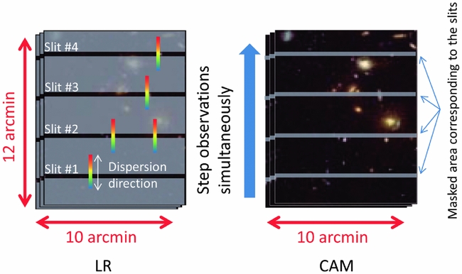
Figure 1. Schematic images of the SMI/LR multi-slit spectroscopic survey with the SMI/CAM slit viewer for pointing reconstruction in creating low-resolution spectral maps. A spatial scan with 90 steps produces a spectral map of 10 arcmin × 12 arcmin area.
3 Survey strategy
As reference surveys, we consider two blind spectroscopic surveys with SMI/LR: (i) a wide survey of a 10 deg2 area aimed at covering various galaxy environments across the cosmic large-scale structure, including (proto-)clusters of galaxies, as well as serendipitously detecting rare luminous galaxies; and (ii) a deep survey of a 1 deg2 area that will cover a wide range of L IR down to those of ordinary star-forming galaxies (i.e., star-formation main-sequence galaxies; Elbaz et al. Reference Elbaz2011) at redshift z ~ 3. Table 1 summarises the parameters of these reference surveys, where the total observation time is assumed to be 600 h in both cases. 600 h is chosen to fit the time allocation plan based on the reference mission scenario for SPICA (Roelfsema et al. Reference Roelfsema2017). The two surveys can be combined by any appropriate ratio, while the total time is kept to be the same. For each pointing of the spatial scan, we take into account a 20-s stabilisation time of SPICA as an overhead. To determine the on-source time, we multiplied the exposure time per step by a factor of 1.5, considering the overlap between each field of view by half a slit width. Most of the popular extragalactic survey fields have enough visibility for the assumed observational time of 600 h (see the sky visibility for SPICA in Figure 2). Hence, the whole areas of 10 and 1 deg2 can be covered either contiguously or separately in principle, but a contiguous mapping would be one of our key advantages over JWST to enhance the ability to perform clustering analyses.
Figure 2. Sky visibility contours of SPICA in units of hours per year. Circles identify popular extragalactic survey fields, NEP (North Ecliptic Pole; Houck, Hacking, & Condon Reference Houck, Hacking and Condon1988; Matsuhara et al. Reference Matsuhara2006), ELAIS-N1 (European Large Area ISO Survey; Oliver et al. Reference Oliver2000), Groth strip (Vogt et al. Reference Vogt2005), GOODS-N/S (Great Observatories Origins Deep Survey; Dickinson, Giavalisco, & GOODS Team Reference Dickinson, Giavalisco, Bender and Renzini2003), COSMOS (Cosmic Evolution Survey; Scoville et al. Reference Scoville2007), UDS (Ultra Deep Survey; Galametz et al. Reference Galametz2013), and AKARI-DFS (AKARI Deep Field South; Matsuura et al. Reference Matsuura2011; Baronchelli et al. Reference Baronchelli2016). Stars indicate the Hubble Space Telescope Frontier Fields (Lotz et al. Reference Lotz2017), which are known to contain high-magnification gravitational lensing clusters of galaxies. We assume that SPICA can observe a ±8° zone along a great circle perpendicular to the solar vector.
Table 1. Survey parameters.
The estimation of the survey spectral sensitivity is based on the latest specifications of SMI/LR, e.g., 5σ; 1-h continuum sensitivities of 25 and 60 μJy at 20 and 30 μm, respectively (Sakon et al. Reference Sakon2016). SMI/CAM has a 5σ; 1-h sensitivity of 13 μJy, the imaging data obtained simultaneously for the wide and deep surveys have the detection limits of 11 and 3 μJy, respectively. Scientifically, SMI/LR spectral data are particularly useful to study star-forming galaxies with the PAH features, while SMI/CAM imaging data are useful to probe dusty AGN by combining other wavelength data as well as the SMI/LR data themselves. As shown below, the SMI/LR surveys will provide so many (~105) PAH spectra of galaxies that we can statistically examine PAH band variations as spectral diagnostics. Technically, given that the absolute flux in the 34 μm band is well calibrated, the spectral data with SMI/LR can be calibrated relative to SMI/CAM at 34 μm as an anchoring point.
The detection limits of the SMI/CAM imaging data are comparable to or less than the confusion limit for SPICA’s 2.5-m diameter telescope (9 μJy at 34 μm; Gruppioni et al. Reference Gruppioni2017). It will be possible to recover fluxes even three times lower than the confusion limit by taking advantage of ancillary data at other wavelengths (preparatory and/or follow-up observations) that will allow us to precisely constrain the position. On the other hand, the SMI/LR spectral data have continuum detection limits of 380 and 110 μJy at 30 μm for the wide and deep surveys, respectively, and thus the confusion makes only very small (<20%) contributions to the underlying continuum in estimating the equivalent widths of dust features. As shown below, in the case of the SMI/LR deep survey, the population density of the detected galaxies reaches 2 × 10⁻² per beam (3.7 arcsec), which indicates that 2% of the galaxies may be blended with another detected galaxy under the assumption that galaxies are uniformly distributed. From the data affected by the blending, it will be possible to extract the PAH spectrum of each galaxy by using the difference in their redshifts, but it will be difficult to recover their continuum components.
It should be noted that, in terms of the limiting flux density for SMI/CAM, the wide and deep surveys are almost equivalent to, and thus consistent with, the Deep Survey and the Ultra-Deep Survey (UDS) described in Gruppioni et al. (Reference Gruppioni2017), respectively. For the 100 deg2 Shallow Survey (SS) proposed in Gruppioni et al. (Reference Gruppioni2017), we plan to conduct additional dedicated photometric surveys using only SMI/CAM, since the spatial step scan for SMI/LR would require an exposure time of ~0.2 s which is too short for the detectors to be operated.
4 Measurement of PAH and dust emission fluxes
We first estimate the limiting fluxes of the PAH features, based on the current specifications of SMI/LR (Kaneda et al. Reference Kaneda2016; Sakon et al. Reference Sakon2016). In the rest frame, we adopt the approximate band widths (Δλ) of 0.08, 0.3, 0.9, 0.4, and 1.4 μm for the PAH features at 3.3, 6.2, 7.7, 11.3, and 17 μm, respectively (Draine & Li Reference Draine and Li2007). In the observed frame, the band widths as well as the central wavelengths of the PAH features change with redshift (Figure 3); from the SMI/LR continuum sensitivities, their limiting fluxes in 1 h (5σ) are calculated to be 8.2 × 10⁻¹⁷, 1.2 × 10⁻¹⁶, 1.8 × 10⁻¹⁶, 1.0 × 10⁻¹⁶, and 1.5 × 10⁻¹⁶ erg s−1 cm−2 at 20 μm, while they are 1.3 × 10⁻¹⁶, 1.9 × 10⁻¹⁶, 2.9 × 10⁻¹⁶, 1.6 × 10⁻¹⁶, and 2.4 × 10⁻¹⁶ erg s−1 cm−2 at 30 μm. Thus, the limiting PAH fluxes vary with redshift by a factor of 1.6 within a range of the redshift where the central wavelength of the corresponding PAH feature is observed at 20 or 30 μm. For simplicity, we adopt the average of the above two fluxes as the 1-h limiting flux f limit for each PAH feature in the following calculation (i.e., f limit = 1.1 × 10⁻¹⁶, 1.5 × 10⁻¹⁶, 2.4 × 10⁻¹⁶, 1.3 × 10⁻¹⁶, and 2.0 × 10⁻¹⁶ erg s−1 cm−2 for the PAH 3.3, 6.2, 7.7, 11.3, and 17 μm features, respectively).
Figure 3. Observed wavelengths of the PAH features as a function of redshift. The striped area indicates the wavelength range covered by SMI/LR.
For pure AGN, we assume that the PAH emission is faint and non-detectable (Moorwood Reference Moorwood1986; Roche et al. Reference Roche, Aitken, Smith and Ward1991); in order to estimate the numbers of the AGN expected to be detected in the SMI spectral surveys, we may be able to utilise the silicate emission features (Hao et al. Reference Hao2005; Sturm et al. Reference Sturm2005). However, unlike PAH, the silicate features can be in either emission or absorption (or both), and also their intrinsic strengths relative to L IR are known to be highly variable from object to object (Hatziminaoglou et al. Reference Hatziminaoglou, Hernán-Caballero, Feltre and Piñol Ferrer2015; Xie et al. Reference Xie, Li and Hao2017). Instead, we use 6 μm continuum emission of hot dust which is typical of AGN just for the purpose of quantitative estimation, the silicate features themselves would be scientifically important to further characterise AGN. To convert the rest-frame 6 μm AGN continuum to that at the observed wavelength, we assume that νF ν is constant. This assumption is reasonable for type 1 AGN because their dust continua are relatively flat around 10–30 μm, exhibiting a broad peak in this range (Shang et al. Reference Shang2011), and still acceptable for type 2 AGN because of similarity in continuum shapes at ~3–30 μm between type 1 and 2 quasars except for the silicate and PAH features (Hiner et al. Reference Hiner2009). Similar to the limiting PAH fluxes, from the SMI/LR and /CAM continuum sensitivities, the 1-h limiting fluxes (5σ) for hot dust emission (νF ν) are 3.7 × 10⁻¹⁵ erg s−1 cm−2 at 20 μm and 6.0 × 10⁻¹⁵ erg s−1 cm−2 at 30 μm for SMI/LR, while they are 1.1 × 10⁻¹⁵ erg s−1 cm−2 for SMI/CAM at 34 μm. For SMI/LR, we again adopt the averages of the two fluxes as the 1-h limiting flux f limit for AGN hot dust emission.
Since pure star-forming galaxies or pure AGN are somewhat extreme cases, we also consider a mixture of them. In the following calculation, we define the three types of galaxies, SF(Star Formation)100%, AGN100% galaxies, and SF50% + AGN50% galaxies. The last type corresponds to a galaxy where a half of L IR is powered by star-formation activity, while the other half is attributed to AGN activity. We consider their detections on the basis of the PAH features or the hot dust continuum emission, when we refer to them as star-forming galaxies (or PAH galaxies as defined below) or AGN, respectively.
For the wide and deep surveys with SMI/LR and /CAM, f limit is scaled with the square root of the on-source exposure time (Table 1), since the SMI/LR sensitivity is limited by background photon noise. To convert f limit to the limiting IR luminosity of a galaxy, L IR, limit, we use the following equation:
 $$\begin{equation}
L_{\rm IR, limit} = 4\pi D_{\rm L}(z)^2\left(\frac{L_{\rm IR}}{L_{\rm PAH\, or\, hot\, dust}}\right)f_{\rm limit},
\end{equation}$$
$$\begin{equation}
L_{\rm IR, limit} = 4\pi D_{\rm L}(z)^2\left(\frac{L_{\rm IR}}{L_{\rm PAH\, or\, hot\, dust}}\right)f_{\rm limit},
\end{equation}$$
where D L(z) is the luminosity distance. To simplify the calculation, we assume that the luminosity of each of the PAH features (L PAH) and the hot dust continuum emission (L hot dust) is proportional to L IR. (In reality, their relative strengths, especially PAH interband ratios, are expected to vary depending on the properties of the interstellar medium in a galaxy, which is also to be studied by SPICA.) The adopted PAH and the monochromatic continuum strengths at 6 μm relative to L IR (i.e., proportionality coefficients) are summarised in Table 2, which are estimated from Spitzer and AKARI near- to mid-IR spectroscopic observations of nearby galaxies (Smith et al. Reference Smith2007; Yamada et al. Reference Yamada2013; Nardini et al. Reference Nardini2009). For the intensities of the PAH 6.2, 7.7, 11.3, and 17 μm features in Smith et al. (Reference Smith2007), we utilised the spline-fitting result but not the result of spectral decomposition (i.e., we excluded the contribution of PAH plateau components), consistently with the above assumption on the widths of the PAH features. For the 6 μm continuum strength, we adopted the value averaged for AGN in nearby ultra-luminous IR galaxies with various geometries of AGN tori (Nardini et al. Reference Nardini2009). For SF50% + AGN50% galaxies, the relative strengths of the PAH features and the hot dust continuum are decreased by a factor of 2 from those of SF100% and AGN100% galaxies, respectively, as shown in Table 2.
Table 2. Strengths of the PAH feature and 6 μm continuum luminosity relative to the total IR luminosity for SF100%, AGN100%, and SF50% + AGN50% galaxies.
a Yamada et al. (Reference Yamada2013).
b Spline-fitting result in Smith et al. (Reference Smith2007).
c Nardini et al. (Reference Nardini2009).
The limiting IR luminosities, L IR, limit, are calculated as a function of redshift, z, for SF100%, SF50% + AGN50%, and AGN100% galaxies. Figure 4 shows the resultant L IR, limit for the wide and deep surveys, where L IR, limit for SF50% + AGN50% galaxies is based on the PAH features. The discontinuity in the plots is caused by appearance or disappearance of the corresponding PAH feature in the SMI/LR spectral range. Here, we consider an edge margin of ±Δλ for inclusion of each PAH feature in the SMI/LR range of 17–36 μm. In the figure, from low to high redshift, the PAH 17, 11.3, 7.7, 6.2 and 3.3 μm features determine the behaviour of L IR, limit as a function of z.
Figure 4. Limiting IR luminosities L IR, limit in Equation (1) for (top) the wide and (bottom) deep surveys, calculated as a function of redshift for the galaxies of SF100% (solid line), SF50% + AGN50% (dot-dashed line), and AGN100% (dashed line), while the horizontal bars show the redshift ranges where multiple major PAH features are available (i.e., their peaks are included).
5 Expected results
5.1. Numbers of galaxies
The luminosity functions used in our calculation are based on those given in Gruppioni et al. (Reference Gruppioni2013) with the Herschel far-IR surveys, where they define the five populations of spiral, starburst, SF-AGN, AGN1, and AGN2, and give the parameters of the luminosity functions for each population. We define the above three types as SF100% = 2/3×(spiral + starburst + SF–AGN), AGN100% = 2/3×(AGN1 + AGN2), and SF50% + AGN50% = 1/2×(SF100% + AGN100%), so that the total numbers are conserved. Note that, by definition, our SF50% + AGN50% is closer to AGN2, while their SF–AGN has the IR luminosity dominated by SF (Gruppioni et al. Reference Gruppioni2013). As a result, we assume significantly more SF–AGN composite systems (i.e., 33% of the total) than suggested in Gruppioni et al. (Reference Gruppioni2013) (e.g., ~15% at z ~ 3), which would give conservative values on the numbers of PAH galaxies in the calculation below. Figure 5 shows the luminosity functions thus derived for different redshift ranges. Above z = 4, we assume the same luminosity functions as those at z = 3–4, since the parameters of the luminosity functions in Gruppioni et al. (Reference Gruppioni2013) are not well constrained in that redshift range.
Figure 5. Luminosity functions for the galaxies of SF100%(solid line), SF50% + AGN50%(dot-dashed line), and AGN100%(dashed line), calculated for the parameters given in Gruppioni et al. (Reference Gruppioni2013).
The number of galaxies at redshifts between z 1 and z 2 with luminosity between L 1 and L 2 is derived as follows:
 $$\begin{equation}
N=\Omega \int _{z_1}^{z_2}\int _{\log L_1}^{\log L_2}\Phi (z,L_{\rm IR})\frac{\text{d}V(z)}{\text{d}z\text{d}\Omega }\text{d}\log L_{\rm IR}\text{d}z,
\end{equation}$$
$$\begin{equation}
N=\Omega \int _{z_1}^{z_2}\int _{\log L_1}^{\log L_2}\Phi (z,L_{\rm IR})\frac{\text{d}V(z)}{\text{d}z\text{d}\Omega }\text{d}\log L_{\rm IR}\text{d}z,
\end{equation}$$
where Ω is the solid angle of the survey area (i.e., Ω = 3.05 × 10⁻³ and 3.05 × 10⁻⁴ sr for the wide and deep surveys, respectively), Φ(z, L IR) is the luminosity function at redshift z and luminosity L IR, and dV(z)/dzdΩ is the comoving volume in a redshift interval dz within a solid angle dΩ. The comoving volume is calculated by adopting the flat universe with the cosmological parameters listed above. If L 1 is fainter than L IR, limit which is estimated in the previous section, we use L IR, limit instead of L 1.
Tables 3 and 4 summarise the numbers of PAH galaxies expected to be detected per bin of the L IR − z plane for the SMI/LR wide and deep surveys, respectively. Here we define the PAH galaxies as a sum of SF100% and SF50% + AGN50% galaxies, and show the contribution of the SF50% + AGN50% galaxies in the parentheses. Considering that typical variations of the PAH feature strengths relative to L IR are ~±30% with 1σ for star-forming galaxies of a near-solar metallicity and in the absence of AGN (Smith et al. Reference Smith2007), we estimate the effect of such variations by changing L IR/L PAH in Equation (1) by ±30%, and find that the total numbers of PAH galaxies in Tables 3 and 4 can vary by ~20% at lower redshift to ~40% at higher redshift. Figure 6 shows the fractions of the PAH galaxies detected with two or three PAH features among those at 6.2, 7.7, 8.6, 11.3, 12.7, and 17 μm. As can be seen in the figure, a majority of the PAH galaxies are detected with multiple PAH features for z ⩽ 3, which is important in order to accurately determine the redshift (see Section 5.2).
Figure 6. Fractions of the galaxies detected with two (stripe) and three PAH features (cross) for the wide survey.
Table 3. Numbers of the PAH galaxies (SF100% and SF50%+AGN50%) expected to be detected in the SMI/LR wide survey. The values in the parentheses are the numbers of SF50%+AGN50% galaxies.
Table 4. Same as Table 3, but for the deep survey.
In Figure 7, we evaluate the effects of systematic changes of the PAH feature strengths relative to L IR. First, we consider the fact that L PAH/L IR decreases with L IR for local ultra-luminous IR galaxies (ULIRGs; Imanishi et al. Reference Imanishi, Nakagawa, Shirahata, Ohyama and Onaka2010; Yamada et al. Reference Yamada2013; Desai et al. Reference Desai2007), while high-z ULIRGs tend to have higer L PAH than local ULIRGs (e.g., Pope et al. Reference Pope2008, Reference Pope2013). Using the L PAH/L IR–L IR relationships at z = 0 and z = 2 given in Shipley et al. (Reference Shipley, Papovich, Rieke, Brown and Moustakas2016), we assume the following three cases for the evolution with redshift, namely that the low-z and high-z relationships change at (1) z = 0.5, (2) 1.0, and (3) 1.5. Figure 7 (top) shows the results for the three cases, from which we find that the systematic changes of L PAH/L IR as a function of L IR and redshift do not significantly affect the numbers of PAH galaxies, most of the galaxies are not that IR-bright. Second, we consider the fact that L PAH/L IR decreases with metallicity (Engelbracht et al. Reference Engelbracht2008). Several works have reported that the metallicities of ULIRGs from the local universe to z ~ 5 are Z = 0.5–1.5 Z⊙ (Rupke, Veilleux, & Baker Reference Rupke, Veilleux and Baker2008; Pereira-Santaella et al. Reference Pereira-Santaella, Rigopoulou, Farrah, Lebouteiller and Li2017; Fadely et al. Reference Fadely2010; Wardlow et al. Reference Wardlow2017; Nagao et al. Reference Nagao2012; Béthermin et al. Reference Béthermin2016). LIRGs at z ~ 2, which have the stellar mass of M⊙ > 109.6M⊙ (Daddi et al. Reference Daddi2007), are expected to have the metallicity of Z > 0.5Z⊙ from the mass-metallicity relation at z = 2 (Maiolino et al. Reference Maiolino2008). Thus, we assume three cases for metallicity, namely Z = 0.8, 0.6, and 0.4 Z⊙. Figure 7 (bottom) shows the result for the effect of the metallicity in these cases, from which we find that the numbers of PAH galaxies can be reduced by a factor of 2–3. There are many other effects that can change L PAH/L IR; for example, it might be harder for PAHs to survive if there is less dust shielding and the radiation field is stronger at high z. Nevertheless, it should be noted that targets that are unique for SPICA are the dusty, obscured populations that are relatively rich with metals and dust.
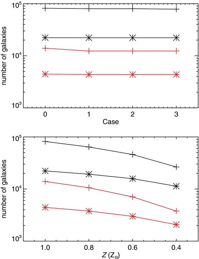
Figure 7. Effects of systematic changes of L PAH/L IR as a function of (top) L IR, redshift, and (bottom) metallicity on the total numbers of PAH galaxies for the wide (black pluses) and deep (black asterisks) surveys. Red symbols are those limited to z > 2. (Top) Cases 1–3 correspond to different assumptions on L PAH/L IR as a function of L IR and redshift (see text for detail), while Case 0 is for the constant L PAH/L IR assumption (i.e., Tables 3 and 4). (Bottom) The changes are calculated based on the metallicity dependence given in Engelbracht et al. (Reference Engelbracht2008).
On the other hand, Tables 5 and 6 summarise the numbers of AGN expected to be detected per bin of the L IR − z plane for the SMI/LR wide and deep surveys, respectively, where we define the AGN as a sum of AGN100% and SF50% + AGN50% galaxies. In the parentheses of the tables, we also show the numbers of the SF50% + AGN50% galaxies as AGN. Note that, to obtain the total numbers of galaxies, we add the values in the tables for the PAH galaxies and AGN, and then subtract the values in parentheses in the tables for the PAH galaxies. Finally, Table 7 lists the numbers of AGN expected to be detected with SMI/CAM in the surveys.
Table 5. Numbers of the AGNs (AGN100% and SF50%+AGN50%) expected to be detected in the SMI/LR wide survey. The values in the parentheses are the numbers of SF50%+AGN50% galaxies.
Table 6. Same as Table 5, but for the deep survey.
Table 7. Numbers of the AGNs (AGN100% and SF50%+AGN50%) expected to be detected with SMI/CAM in the wide survey. The values in the parentheses are those with SMI/CAM in the deep survey.
The tables clearly show that a huge number of galaxies are foreseen to be detected in the SMI surveys. In particular, from Tables 3, 5, and 7, we find that the wide survey would produce ~5 × 10⁴ spectra of PAH galaxies at z > 1, among which ~1.4 × 10⁴ spectra would come from galaxies at z = 2–4, as well as ~2 × 10⁴ spectra of AGN at z > 1, while the slit viewer would detect more than 2 × 10⁵ dusty AGN at z > 1. On the other hand, Tables 4 and 6 show that the deep survey reaches luminosity levels of so-called star-formation main sequence galaxies (e.g., L IR ~ 1 × 10¹² L⊙ at z ~ 3) with a fair margin. Thus, with the sample size and depth in the tables, we will be able not only to establish robust rest-frame mid-IR spectral samples as a function of z and L IR, but also to examine PAH and silicate band variations as spectral diagnostics of the physical conditions in the star-forming regions and the nuclei of galaxies with the help of other wavelength spectral data.
5.2. Characterisation of PAHs
We have created simulated SMI/LR PAH spectra in order to confirm the result obtained in the previous subsection, and also the applicability of the PAH features to determine the redshift and to characterise the PAHs in a galaxy. The model spectrum was taken from that of typical Galactic diffuse PAH emission (Draine & Li Reference Draine and Li2007) plus an M82-like continuum approximated by a power-law component. We assumed galaxies at redshift z = 3 with three levels of total IR luminosities, L IR = 1 × 10¹², 3 × 10¹², and 1 × 10¹³ L⊙. Then L PAH7.7 is determined and fixed according to the relation in Table 2, while L PAH6.2 and L PAH8.6 are allowed to vary by a factor of 3 relative to L PAH7.7. The latter reflects a possible systematic difference in the properties of PAHs in galaxies at high-z when compared to those in the nearby universe as well as their intrinsic variations from galaxy to galaxy.
Figure 8 shows examples of the simulated spectra of SF100% and SF50% + AGN50% galaxies at z = 3 for the SMI/LR deep survey. As for the AGN continuum, we utilised an AGN spectral template (Polletta et al. Reference Polletta2007) and scaled the amplitude so that the IR luminosity integrated from 8 to 1 000 μm reaches a specified value (i.e., 0.5 × L IR). A Nyquist sampling for R = 50 resolution was adopted, adding white noise with amplitude based on the continuum sensitivity expected for the deep survey (~100 μJy, 5σ). In order to fit the spectra, we used PAHFIT (Smith et al. Reference Smith2007), assuming a power-law continuum and an extinction curve with a screen configuration (Kemper, Vriend, & Tielens Reference Kemper, Vriend and Tielens2004). Free parameters are the normalisations of the PAH features, the normalisation, and the index of the power-law continuum, and the extinction. PAHFIT assumes that the PAH 7.7 and 8.6 μm features are the complexes consisting of 7.4, 7.6, and 7.8 μm sub-features and 8.3 and 8.6 μm sub-features, respectively. In both generating and fitting the simulated spectra, we fixed the relative intensity ratios among the sub-features at typical values for each complex (Draine & Li Reference Draine and Li2007), but allowed the PAH 8.6 μm feature to vary with respect to the PAH 7.7 μm feature.
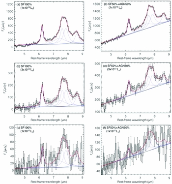
Figure 8. Simulated SMI/LR spectra of a galaxy at z = 3 for the deep survey, SF100% on the left and SF50% + AGN50% on the right-hand side with L IR denoted in each panel. Solid curves indicate best-fit results with PAHFIT.
First, we take results of spectral fitting for SF100% galaxies. We confirm that the redshift is determined with the accuracies of 2, 0.7, and 0.3% for galaxies with L IR of 1 × 10¹², 3 × 10¹², and 1 × 10¹³ L⊙, respectively. Figure 9a shows a correlation plot between the output (measured) and input (simulated) values of L PAH (≡ L PAH6.2 + L PAH7.7 + L PAH8.6). From the figure, we find that L PAH is determined with the accuracies of 13% (bias: 0.8%), 5% (1%), and 3% (0.3%) for galaxies with L IR of 1 × 10¹², 3 × 10¹², and 1 × 10¹³ L⊙, respectively; here and hereafter, the accuracy is defined by the standard deviation of the absolute values of the differences between the input and output divided by the input values, while the bias is the systematic difference between the input and output values. Hence, the SMI/LR surveys can estimate the redshift very precisely, and also measure L PAH of so-called main-sequence galaxies at z = 3 (~1 × 10¹² L⊙). Figures 9b and 9c show correlation plots between the input and output values of L PAH6.2/L PAH7.7 and L PAH8.6/L PAH7.7, respectively. From the figure, we find that L PAH6.2/L PAH7.7 is determined with the accuracies of 31% (bias: −0.8%), 9% (0.2%), and 4% (−0.3%), while L PAH8.6/L PAH7.7 is determined with 47% (4.3%), 13% (1%), and 6% (−1%) for galaxies with L IR of 1 × 10¹², 3 × 10¹², and 1 × 10¹³ L⊙, respectively. Thus, the result also demonstrates applicability of those features to characterise PAHs in galaxies at z ~ 3.
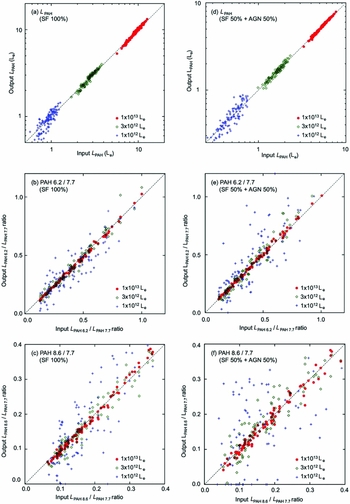
Figure 9. Correlation plots between output (measured) and input (simulated) values of (a), (d) L PAH, (b), (e) L PAH6.2/L PAH7.7 and (c), (f) L PAH8.6/L PAH7.7 of galaxies at z = 3 for the deep survey, SF100% on the left and SF50% + AGN50% on the right-hand side. The dashed line in each panel corresponds to y = x.
For SF50% + AGN50% galaxies, the above accuracies are degraded to 3, 0.8, and 0.6% for the redshift, 19% (bias: 2%), 8% (1%), and 3% (0.5%) for L PAH, 43% (9%), 12% (−2%), and 4% (−0.4%) for L PAH6.2/L PAH7.7, 85% (18%), 24% (8%), and 8% (0.5%) for L PAH8.6/L PAH7.7 for galaxies with L IR of 1 × 10¹², 3 × 10¹², and 1 × 10¹³ L⊙, respectively. The degradation is caused by the decrease in L PAH/L IR for SF50% + AGN50% galaxies by a factor of 2 from that for SF100% galaxies. Figure 10 shows a correlation plot for the PAH equivalent width values used to estimate the star-formation contribution to the total L IR of a galaxy. We find that the accuracies of the equivalent widths are 34% (bias: −4%), 10% (−1%), and 4% (−0.1%) for the PAH 6.2 μm and 21% (1%), 7% (1%), and 3% (0.2%) for the PAH 7.7 μm features. Hence, we can estimate the relative proportions of the AGN and star-formation contributions to L IR in galaxies down to a luminosity level of ~1 × 10¹² L⊙, although we need L IR > 3 × 10¹² L⊙ to characterise the PAH emission bands.
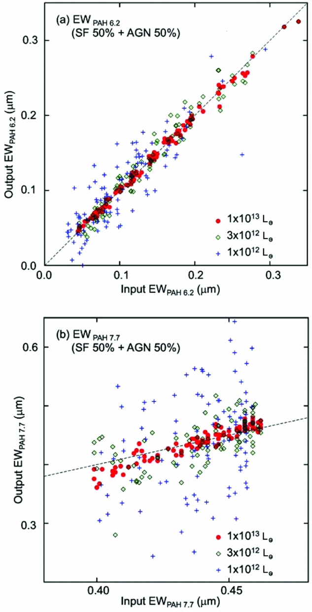
Figure 10. Correlation plots between output (measured) and input (simulated) values of (a) the PAH 6.2 μm and (b) 7.7 μm equivalent widths of SF50% + AGN50% galaxies at z = 3 for the deep survey. The dashed line in each panel corresponds to y = x.
In the above cases, three PAH features are used for the redshift determination. Here we estimate the degradation of their accuracies as the number of PAH features decreases. In the SF100% case, if we use only two features (6.2 and 7.7 μm), the accuracies are degraded to 2, 0.9, and 0.3% for L IR = 1 × 10¹², 3 × 10¹², and 1 × 10¹³ L⊙, respectively. If we use only one feature (6.2 μm), they are 3, 1, and 0.5%. In the SF50% + AGN50% case, the accuracies are degraded to 5, 1, and 0.7% in the case of two features, while they are 10, 2, and 0.8% in the case of one feature. Taking these accuracies and the result in Figure 6 into account, we estimate that the redshifts are determined with an accuracy of ⩽2% for 84% of the SF100% galaxies and 68% of the SF50% + AGN50% galaxies at z = 2–4.
5.3. Synergies with SAFARI and future large facilities
The SMI blind surveys will provide us with unbiased, uniform, and statistically significant numbers of samples for follow-up spectroscopy with the SPICA far-IR instrument, SAFARI (and also SMI/MR or /HR, if necessary). Since the field of view of SAFARI is rather narrow (Pastor et al. Reference Pastor2016), the integrated survey strategy is important for defining unbiased studies. The spectral datasets obtained with SMI/LR will enable us to estimate redshifts, IR luminosities, and fractional AGN luminosities of follow-up candidates, and thus to plan strategic observations with SAFARI. Then SAFARI would provide information on the properties of atomic and ionic gas in a galaxy based on fine-structure line diagnostics (e.g., [S iii] 18, 33 μm, [O iv] 26 μm, [Si ii] 35 μm, [O iii] 52, 88 μm, and [N iii] 57 μm) (Spinoglio et al. Reference Spinoglio2012, Reference Spinoglio2017; Fernández-Ontiveros et al. Reference Fernández-Ontiveros2016), which is complementary to the information on dust features provided by SMI (e.g., PAHs, silicates).
Beyond z = 1, some of the PAH 6.2, 7.7, 11.3, and 17 μm features fall outside of the SMI range, but will be covered by SAFARI. Figures 11 a–d visualise such complementarity between SMI and SAFARI in detecting the PAH 6.2, 7.7, 11.3, and 17 μm features, respectively. The contour maps show the number densities of the PAH galaxies expected to be detected by the SMI/LR deep survey, while the colour maps show those detectable with a SAFARI 1-h pointing spectroscopy. From the figure, we can confirm that the SMI and SAFARI domains are connected smoothly to each other. Hence, the integrated SAFARI and SMI observations allow us not only to detect the discrete PAH features but also to characterise the PAH emission in distant galaxies for the first time.
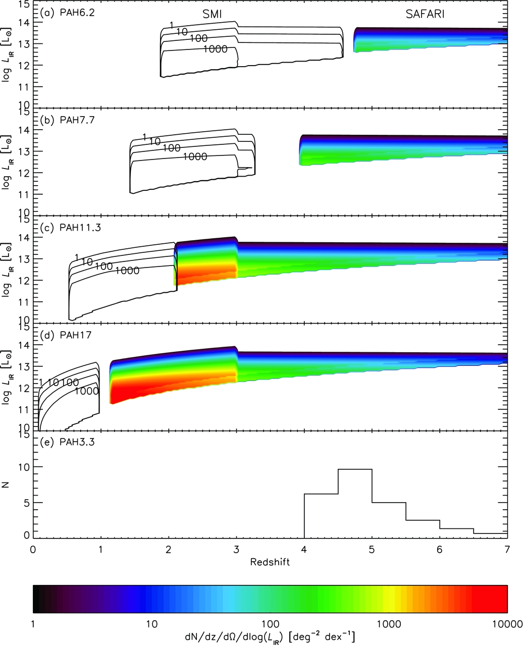
Figure 11. Number densities of PAH galaxies per unit redshift, per deg2, and per unit dlog(L IR) detectable with SAFARI (colours) in 1-h exposure using (a) the PAH 6.2, (b) 7.7, (c) 11.3, and (d) 17 μm features. The result of the SMI/LR deep survey is shown together with contours of four levels (1, 10, 100, 1 000 per unit redshift, unit deg2, and unit dlog(L IR)). (e) Number of galaxies expected to be detected in the PAH 3.3 μm feature with SMI/LR in the deep survey.
SMI provides high-redshift samples beyond z = 4 where the PAH 3.3 and 6.2 μm features are available at z > 4.3 and z = 4–4.6, respectively, within the wavelength range of SMI/LR. For example, the expected number of galaxies beyond z = 4 is ~170 for the deep survey (see Table 4), most of which may be important targets to perform follow-up observations with SAFARI. In particular, the PAH 3.3 μm feature (and possibly aliphatic sub-features at 3.4–3.6 μm) could be a very powerful probe of high-redshift dusty galaxies, because there are no upper limits on the coverage of redshift practically, and its intrinsic bandwidth matches very well the instrumental spectral resolution (R = 50–120) of SMI/LR. It should be noted that, at z > 5, where the observed wavelength of the PAH 3.3 μm feature exceeds 20 μm, the R = 50 continuum sensitivity of SMI/LR surpasses that of JWST/MIRI [e.g., 3 and 10 times higher at 20 and 28 μm, respectively, according to Glasse et al. (Reference Glasse2015)]. However, the PAH 3.3 μm feature is relatively weak as compared to the other PAH features (see Table 2), and therefore galaxies must be sufficiently IR bright. Nevertheless, as shown in Figure 11e, our calculation indicates that we can expect to detect ~30 galaxies at z = 4–7 in the PAH 3.3 μm feature, and even more if we consider gravitational-lensing effects (Egami et al. in preparation). Although the PAH 3.3 μm feature is relatively narrow, its profile is still resolved with SMI/LR, and thus even detecting a single feature may enable us to estimate the redshift (with the help of the comparably bright hydrogen recombination line Brα at 4.05 μm and possibly the sub-features at 3.4–3.6 μm and the H2O ice feature at 3 μm.) Since SAFARI can measure rest-frame mid-IR PAH features while ALMA (Atacama Large Millimeter/submillimeter Array) can measure dust continuum emission, follow-up observations of those targets with SAFARI and ALMA are of particular importance to study organic matter chemistry and dust physics in the early universe.
In the context of a study of PAHs, we can expect a strong synergy between JWST and SPICA: JWST can detect all near- and mid-IR features of PAHs in the nearby universe, while SPICA can access those except the 17 μm feature only at z > 1. JWST will be able to reveal detailed physics and chemistry of PAHs in the nearby universe and to establish the PAH features as spectral tools. Then, that knowledge can be applied to studies of galaxies at high-z with SPICA. Hence, the roles of JWST and SPICA are complementary to each other in studying PAHs in the near and far universe. On the other hand, in terms of dusty AGN, we can expect a strong synergy between Athena (Advanced Telescope for High ENergy Astrophysics) and SPICA. The wide field-of-view of Athena enables efficient surveys of classical AGN, including both types 1 and 2. There is compelling evidence that the fraction of buried AGN increases with L IR (Lee et al. Reference Lee, Hwang, Lee, Kim and Lee2012), and the SMI surveys are very sensitive to the buried AGN which Athena cannot easily detect due to heavy absorption (Gruppioni et al. Reference Gruppioni2017). The strategy of deep X-ray follow-up observations of SMI-selected AGN at high redshift will work very efficiently, because X-ray spectra above rest-frame 10 keV will provide crucial information on the poorly studied nuclear environments of obscured AGN (Stern et al. Reference Stern2014; Piconcelli et al. Reference Piconcelli2015). Hence, SPICA and Athena play roles complementary to each other in revealing contribution of both classical and buried AGN to L IR.
6 Additional science
It should be noted that future cosmological surveys with SMI/LR would simultaneously provide an unbiased, statistically significant view on nearby objects like foreground stars and galaxies as well. Among them, the LR spectra of debris disks in main-sequence stars will be one of the most important by-products to take advantage of the high spectral survey speed of SMI/LR. We estimate below the number of the debris disks expected to be detected by the SMI/LR wide survey.
First, based on the AKARI all-sky survey at 18 μm (Ishihara et al. Reference Ishihara2010), we estimate that a total number of 1.1 × 10⁴ F, G, and K-type main-sequence stars would be detected at 20 μm by the SMI/LR wide survey, considering the improvement in the sensitivity from AKARI to SPICA. Here, we assume an isotropic distribution of stars with 400 pc in the height of the Galactic disk in the solar neighbourhood (Siebert, Bienaymé, & Soubiran Reference Siebert, Bienaymé and Soubiran2003). AKARI detected debris disks of luminosity levels ~1 × 10³ times higher than that of our zodiacal cloud (L Zodi ≃ 1 × 10⁻⁷ L⊙; Nesvorný et al. Reference Nesvorný2010) in an unbiased manner, and revealed that ~10% of the stars possess debris disks at that luminosity threshold (Ishihara et al. Reference Ishihara2017). Then we estimate what fraction of the main-sequence stars detected in the SMI survey possess detectable debris disks, assuming a luminosity function of debris disks, which is unknown for faint disks and thus could be determined by SPICA.
Estimating the limiting flux density of dust emission from debris disks is not straightforward, because we have to consider the underlying photospheric continua of the central stars. As a rough estimation, we adopt the limiting flux density of 200 μJy at 20 μm, which is 10 times worse than the 5σ continuum sensitivity of SMI/LR in a low background, this flux density corresponds to the luminosity of a debris disk with L Zodi at a distance of 10 pc for a 200 K blackbody continuum emission. Figure 12 shows the numbers of the debris disks estimated with the above limiting flux density under the assumption that the (cumulative) existence probability of debris disks with >1 × 10³ L Zodi and >1 L Zodi are 10% (based on the AKARI results), and 100%, respectively. We interpolated the existence probability function between 1 L Zodi and 1 × 10³ L Zodi by two types of curves as shown in the lower panel of Figure 12, and counted the numbers of debris disks in the luminosity range of 1 L Zodi to 1 × 10⁴ L Zodi. As a result, the total number is in the 1 800–2 600 range, depending on the types of the existence probability curves. The probability of signal blending with galaxies is very low, the number of galaxies expected to be detected with the above limiting flux density is calculated to be about 2 × 10⁻⁴ per beam (3.7 arcsec) of SMI/LR in the wide survey.
Figure 12. Numbers of the debris disks of F, G, and K-type main-sequence stars expected to be detected by the SMI/LR wide survey, which are estimated based on the result of the AKARI all-sky survey as a function of the disk luminosity. The Spitzer summary result is also shown for comparison (Chen et al. Reference Chen2014). The lower panel shows the assumed existence probability curves of debris disks as a function of the disk luminosity, the solid one of which is used to obtain the result of the upper panel. The dashed curve is also considered to estimate the uncertainty of the result.
Our simple calculation suggests that we can detect faint debris disks of 5–10 L Zodi levels in principle. It is a significant step forward to statistically understanding the evolution of debris disks towards our zodiacal cloud analogues, with fainter and presumably more common disks than those in the previous studies (e.g., Chen et al. Reference Chen2014). However, in order to detect such faint debris disks, we must determine the underlying stellar continuum with 0.1–1% calibration accuracy and stability, which is in practice rather difficult. One possibility is to use different spectral shapes between the Rayleigh–Jeans stellar continuum and thermal dust emission, especially dust bands if present (e.g., silicate features; Fujiwara et al. Reference Fujiwara2010; Olofsson et al. Reference Olofsson2012). Hence, the SMI/LR wide survey could characterise the properties of many debris disks and potentially detect faint debris disks similar to our zodiacal cloud.
7 Summary
We have evaluated the capability of LR mid-IR spectroscopic surveys of galaxies with SMI onboard SPICA. For instance, a wide survey of 10 deg2 area in 600 h would provide ~5 × 10⁴ PAH spectra from galaxies at z > 1, would detect more than 2 × 10⁵ dusty AGN at 34 μm with the slit viewer, and at the same time, is expected to obtain more than 1 × 10⁴ spectra from main-sequence stars of F, G, and K types in the foreground and at least 1 × 10³ debris disks among them. Thus, the SMI/LR-CAM surveys are capable to efficiently provide us with unprecedented large spectral and photometric samples that would cover very nearby planet-forming stars to distant star-forming galaxies and AGN especially in the unexplored 30–40 μm wavelength regime. These samples would be crucial as follow-up candidates to be further studied with SPICA on such major science topics as described in a series of the relevant papers in this volume (Spinoglio et al. Reference Spinoglio2017; Gonzalez-Alfonso et al. Reference González-Alfonso2017; Fernández-Ontiveros et al. Reference Fernández-Ontiveros2017; Gruppioni et al. Reference Gruppioni2017; van der Tak et al. Reference van der Tak2017).
ACKNOWLEDGEMENTS
This paper is dedicated to the memory of Bruce Swinyard, who unfortunately passed away on 2015 May 22 at the age of 52. He initiated the SPICA project in Europe as first European PI of SPICA and first design lead of SAFARI.
We thank all the members of SPICA Science Working Group and the SMI consortium for their continuous discussions on science case and requirements for SMI. We are especially grateful to the board members of SPICA Science Case International Preview (Michael Rowan-Robinson, Martin Bureau, David Elbaz, Peter Barthel, Anthony Peter Jones, Martin Harwit, George Helou, Kazuhisa Mitsuda) and JAXA’s SPICA International Science Advisory Board (Philippe Andre, Andrew Blain, Michael Barlow, David Elbaz, Yuri Aikawa, Ewine van Dishoeck, Reinhard Genzel, George Helou, Roberto Maiolino, Margaret Meixner, Tsutomu Takeuchi) for giving us invaluable comments and advice. The optical/mechanical designing activities of SMI to fulfill the science requirements are funded by JAXA within the framework of the SPICA preproject in Phase A1.


