


Introduction
Shape grammars have been used successfully to explore design spaces in various design contexts (Strobbe et al., Reference Strobbe, Pauwels, Verstraeten, De Meyer and Van Campenhout2015). They are used to both analyze existing styles and generate new designs. Generative capability and shape emergence are two aspects of shape grammars that make them appealing to designers, and many implementations have illustrated how designers might take advantage of this generative capability (Chase, Reference Chase2010). However, there is a range of shape emergence capabilities in these implementations and shape emergence is generally restricted, in each implementation, to particular kinds of shape. This paper demonstrates the potential of lattice structures to improve the shape emergence capabilities of U 13 shape grammar implementations. Shape emergence algorithms in current implementations are complex, in part, because computational geometry and shape computation are considered simultaneously. This paper provides a mechanism where lattices are used to reduce this complexity by decoupling computational geometry (needed for the geometrical operations associated with specific grammars used in the generation of new shapes) and shape computation (needed for sub-shape detection and the application of rules). A prototype implementation of an interpreter kernel has been built and applied to two well-known shape grammars: Stiny's triangles grammar (Stiny, Reference Stiny1994) and Jowers and Earl's trefoil grammar (Jowers & Earl, Reference Jowers and Earl2010). Early results are promising with more applications, for wider evaluation, and integration with suitable user interfaces as important next steps.
Background and related works
Existing shape grammar implementations that support emergence
Computer implementation of shape grammars with shape emergence is challenging (Chase, Reference Chase2010; McKay et al., Reference McKay, Chase, Shea and Chau2012; Yue & Krishnamurti, Reference Yue and Krishnamurti2013). Five shape grammar implementations that support shape emergence are considered here (Table 1). They were selected because technical details on their use of basic elements and how they support shape emergence are readily available in the literature. The first three implementations (Krishnamurti, Reference Krishnamurti1981; Chase, Reference Chase1989; Tapia, Reference Tapia1999) use two endpoints to describe straight lines in two dimensions (U 12). The other two (Li et al., Reference Li, Chau, Chen, Wang, Chang, Champion, Chien and Chiou2009; Jowers & Earl, Reference Jowers and Earl2010) use circular arcs and curves, respectively, with the latter using parametric Bézier curves or their variations to describe curves.
Table 1. Basic elements of selected shape grammar implementations that support emergence
The goal of this research is to provide a shape grammar implementation method that is extensible to a wide range of curves (any that can be represented as a rational Bézier curve) and dimensionalities. Such implementations are needed if shape grammars are to be used as generative design tools in product development processes. For this reason, implementations that support emergence in parametric grammars using rectilinear shapes, for example, Grasl and Economou (Reference Grasl and Economou2013) are not included. Other implementations that allow emergence, such as those based on bitmap representations (Jowers et al., Reference Jowers, Hogg, McKay, Chau and de Pennington2010), are not included because they represent shapes using discrete pixels, essentially U 02 which, again, limits their extensibility.
Shape grammar interpreter (Krishnamurti, Reference Krishnamurti1981), uses straight lines as basic elements, but lines parallel with the y-axis are treated differently to lines that are not. Chase (Reference Chase1989) reports further progress on the consideration of automatic subshape recognition of shapes consisting of straight lines in any orientation and GEdit (Tapia, Reference Tapia1999) presents users with a visualization of choices of how shape rules based on straight lines can be applied. Shape grammar synthesizer (Chau et al., Reference Chau, Chen, McKay, de Pennington and Gero2004; Li et al., Reference Li, Chau, Chen, Wang, Chang, Champion, Chien and Chiou2009) uses straight line segments and circular arcs in three dimensions and Jowers and Earl (Reference Jowers and Earl2011) used quadratic Bézier curve segments as basic elements in two dimensions. Each of these implementations considers computational geometry and shape computation simultaneously with special cases used to cater for the different geometric combinations in the shape computation process. As a result, extending any of these [five] implementations to cover more shapes and/or dimensionalities would be challenging because of the growth in the number of special cases needed, which is in the order of an n 2 problem. The approach proposed in this paper explores the potential of lattice structures to decouple steps in a shape computation from the geometrical operations associated with specific grammars. This removes the need for the treatment of special cases and so makes the method more extensible because it transforms it into the order of an n problem. A fuller description of the proposed approach and a detailed comparison with Jowers and Earl's method are included in later sections of this paper.
In the 1999 NSF/MIT Workshop on Shape Computation, one of the four sessions was devoted to computer implementations of shape grammars (Gips, Reference Gips1999). One discussion area considered whether a single implementation could support both shape emergence and parametric grammars. It was acknowledged that significant research challenges needed to be resolved before both could be achieved. Nearly two decades later, we can find the most substantial grammars, especially in architectural design, are parametric and can be used to both describe styles and generate new designs. On the other hand, Grasl and Economou (Reference Grasl and Economou2013) made significant headway to support shape emergence in parametric grammars using straight lines.
Graph grammar implementations for spatial grammars
Graph grammars are a popular approach for the analysis of styles in architectural and other kinds of design (Rudolph, Reference Rudolph and Gero2006; Grasl, Reference Grasl2012). Grasl and Economou (Reference Grasl and Economou2013) used graphs and a meta-level abstraction in the form of a hypergraph. Graph grammars also offer tractable implementations of shape grammars, in that they make use of established algorithms for graph operations and rules. The graphs describe shapes in terms of the incidence of shape elements. A range of incidence structures are used in implementations. Each depends on the underlying parts chosen to represent a shape. These range from elements corresponding to the polygons of edges in the shape to incidence between line elements. Substructures in these incidence structures can correspond to emergent shapes. Graph type incidence structures represent binary relations among elements. Higher dimensional relations, where several elements may be mutually related, can be represented by hypergraphs (Berge, Reference Berge1973). This correspondence is used to good effect by Grasl and Economou (Reference Grasl and Economou2013) in their application of graphs and hypergraphs to enable shape emergence in straight line shapes in U 13. The graph grammar implementations allow recognition of substructures which may correspond to emergent shapes.
Terminology and the application of lattice theory
The approach proposed in this paper is used for each rule application in a given shape computation process where the rule is applied under affine transformations except shears. For this reason, there are two inputs: a shape rule and an initial shape. Lattice structures are used because of their ability to represent all possible combinations of the collection of shape elements that form the initial shape and could result from the application of the rule. Each node in the lattice represents either a shape element that is a maximal shape (and so not divisible in the shape computation step) or an aggregation of such elements including both sub-shapes that are parts of the initial shape description and emergent shapes.
Terminology
A partially ordered set (poset) has a binary ordering relation that is reflexive, anti-symmetric, and transitive conditions. The binary relation ≤ can be read as “is contained in”, “is a part of,” or “is less than or equal to” according to its particular application (Szász, Reference Szász1963). When Hasse diagrams (Figs. 8, 12) are used to represent posets, the ordering relation is represented by a line adjoining two nodes that have different vertical positions, where the lower node is a part of the upper one. Their horizontal positions are immaterial. Visual representations of lattices, in the form of Hasse diagrams are used in this paper to illustrate how the use of lattices can decouple computational geometry and shape computation aspects. Hasse diagrams are not required in actual use where it is sufficient to store and relate all elements of a lattice symbolically.
A lattice, in our case, is a poset of shapes. Each node is a shape in algebra U ij, which is a subshape of the initial shape for the given rule and has a set of basic elements (Stiny, Reference Stiny1991). Each basic element is a shape in its maximal representation (Krishnamurti, Reference Krishnamurti1992) and can be divided into its relatively maximal parts. These relatively maximal parts are a segmentation of non-overlapping parts based on the element's intersections with other basic elements in the initial shape. Any two relatively maximal parts of a basic element have no common parts. However, these relatively maximal parts are not in maximal representation and can be recombined to form the original basic element.
Lattice theory
Ganter and Wille (Reference Ganter and Wille1999) use lattices as a basis for formal concept analysis which enables the definition of ontologies (Simons, Reference Simons1987) induced on sets of objects through their attributes. Numerous applications are reported in the literature especially in the Concept Lattice and Their Applications conference series (Ben Yahia & Konecny, Reference Ben Yahia and Konecny2015; Huchard & Kuznetsov, Reference Huchard and Kuznetsov2016) which ranges across architecture, engineering and healthcare, and in The Shape of Things workshop series (Rovetto, Reference Rovetto, Kutz, Hastings, Bhatt and Borgo2011; Ruiz-Montiel et al., Reference Ruiz-Montiel, Mandow, Pérez-de-la-Cruz, Gavilanes, Kutz, Hastings, Bhatt and Borgo2011). Aggregations of objects in a formal concept lattice [an ontology] allow parts of the aggregation, the objects, to be recategorized using their attributes. For example, cats, dogs, and snails may be the objects that are initially grouped as family pets; defining them in a formal concept lattice could allow them to be recategorized as mammals and mollusks for a different purpose. In this paper, we use lattices in a different way: to provide a symbolic representation of an initial shape in the context of a shape rule in terms of their common parts. The use of lattices in shape applications is less common but there are examples in the literature. For example, March (Reference March1983, Reference March1996) used lattices to describe geometric shapes, Stiny (Reference Stiny1994, Reference Stiny2006) used a lattice of parts to describe continuity in a sequence of shape rule applications and Krstic (Reference Krstic2010, Reference Krstic and Gero2016) used lattices in shape decompositions.
A lattice (Szász, Reference Szász1963; Grätzer, Reference Grätzer1971) is a poset such that the least upper bound and the greatest lower bound are unique for any pair of nodes. As a result, for any pair of shapes (represented as nodes) in the lattice, there exists a unique least upper bound and a unique greatest lower bound. This property is exploited in the detail of the implementation when calculating, for a given shape, its parents, children, and siblings. A lattice satisfies idempotent, commutative, associative, and absorption laws and is one of the fundamental abstract algebra constructs. In this paper, the nodes in a lattice are used to represent shapes in algebra U 13, and the binary ordering relation ≤ is the subshape relation. In essence, we use the lattice to create a temporary set grammar based on the initial shape and the rule that is to be applied.
The lattices we use are complemented distributive lattices because, for any complemented lattice, the complement of any node always exists and is unique, and for any distributive lattice, the join of any two nodes always exists and is unique. A complemented distributive lattice is a Boolean algebra and these properties allow shape difference and sum operations to be defined in terms of complements and joins. We exploit this as a basis for set grammar computation of the initial shape and the shape rule represented by the lattice.
Proposed method
The crux of the proposed method is to reduce a shape grammar to a set grammar for each application of a rule, A → B, by decomposing an initial shape, C, into a finite number of shape atoms in the context of the left-hand side of the rule, A. Each atom is a combination of relatively maximal [shape] parts of C. Since shape C has a finite number of atoms, a corresponding temporary set grammar can be used to compute the shape difference operations needed to calculate the complements C − t(A) symbolically without considering the actual geometry of either C or A. For any given lattice node that is a t(A), its complement C − t(A) can be derived from the lattice.
For the purpose of describing one step of a shape computation, which involves the application of a shape grammar rule, a temporary set grammar (represented as a lattice) is derived from the rule and the initial shape. This set grammar is only valid for one step of a shape computation. [Shape] atoms, which consist of a number of relatively maximal parts, are nodes in the lattice. A node represents a shape which is composed of atoms. An atom is a non-decomposable shape during this step of the shape computation. All possible matching t(A) and their complements C − t(A) are also nodes in the lattice.
A four-step process (Fig. 1) is proposed for applying a shape rule which may have many potential applications to the initial shape. Aspects of computational geometry and shape computation are decoupled. The computational geometry of basic elements is used in steps 1 and 4, and shape computation in the second and the third. Steps 2 and 3 use the shape algebra of the set grammar represented by the lattice without considering actual geometry. This is possible because atoms of the set grammar are relatively maximal to one another.
Fig. 1. Proposed method.
Step 1: divide basic elements into parts
First, basic elements (Fig. 2b) of an initial shape C (Fig. 2a) are divided into relatively maximal parts (Fig. 2c) under transformations using their registration points (Krishnamurti & Earl, Reference Krishnamurti and Earl1992). These parts are regrouped to form atoms (Fig. 2d). These atoms of C are indivisible during an application of a shape rule A → B under any valid transformation t (Fig. 2e–g). The left-hand side A of the rule determines the decomposition of C.
Fig. 2. Dividing shape C into relatively maximal parts and recombine them to form atoms.
Registration points are endpoints, control vertices, and intersection points of basic elements of shapes A and C. Three non-collinear registration points from each shape determine a three-dimensional (3D) local coordinate frame that consists of an origin and three orthogonal unit vectors. Each pair of these coordinate systems determines a candidate transformation. This transformation denotes translation, rotation, mirror, proportional scaling or a combination of them. All valid transformations that satisfy the subshape relation t(A) ≤ C are found by an exhaustive search, provided there are at least three non-collinear registration points.
There are other approaches that require less than three registration points to define a coordinate frame. One example is matching Stiny's (Reference Stiny2006, p. 261) that has two or more intersecting lines. It uses only one registration point but requires a pre-defined scaling factor. There is potentially an infinite number of matches which present problems for automatic shape recognition when one wishes to enumerate all possible matches. Another example is two non-intersecting non-parallel lines in three dimensions (Krishnamurti & Earl, Reference Krishnamurti and Earl1992). Their shortest perpendicular distance gives two registration points and a length for an automatic scaling calculation. Any endpoint on these lines gives the third registration point. Details are expanded in the subsection “Determination of curve-curve intersections”. A logical extension to two more cases of this approach would be the use of the shortest perpendicular distance between a straight line and a circular arc, or two circular arcs. Each case is slightly different in the determination of three registration points. In principle, we could have incorporated the latter approach but did not for the sake of simplicity in demonstrating the core idea of the proposed method.
Each matching t(A) is then used to operate on C iteratively to divide the basic elements of C into its parts unless the two shapes are identical. Since both shapes t(A) and C are in maximal representation, each basic element in t(A) is a subshape of one and only one basic element in C. Since that basic element in t(A) is a proper subshape of the element of C, the element of C is divided into two or three parts: the match and its complement where the complement could be in one part or two discrete parts depending on the spatial relation between that basic element of t(A) and the corresponding element in C. For example, u 2 (Fig. 2c) is a subshape of U (Fig. 2b), and its complement consists of two relatively maximal parts u 1 and u 3 (Fig. 2c).
The next iteration looks for a match of another basic element of t(A). It is similar to the first iteration except that some basic elements of C may be already divided into their relatively maximal parts. Each relatively maximal part of C could be further subdivided if its spatial relation with another basic element in t(A) demands it. The process is repeated until all basic elements in this t(A) are either matched or not. Shape C is then partitioned into a set of relatively maximal parts.
Certain combinations of these relatively maximal parts could be either entirely a subshape of all t(A) or not at all under every valid transformation. Each combination is regrouped as an atom. Putting all atoms together results in a visual equivalent of C but with a different underlying representation. In addition, certain combinations of these atoms could produce visual equivalents of each and every t(A).
Step 2: generate a lattice of shape C
The atoms from step 1 are then used, in step 2, to construct a lattice structure to represent C, where each atom and its complement are nodes. Furthermore, the shape C is the supremum of this lattice, and an empty shape its infimum. More importantly, all matching t(A) and their complements C − t(A) are nodes in the lattice. This lattice structure representation, in effect, converts the shape grammar into a temporary set grammar for one shape rule application. It is important to stress that all t(A) and their complements C − t(A) are represented in their relatively maximal parts but not in maximal representation.
Step 3: select a matching left-hand side t(A)
Using the set grammar, for any given rule in the shape grammar, a shape difference operation is used to produce an intermediate shape, C − t(A). This is achieved by navigating the lattice to find all t(A) under Euclidean transformations. Consequently, a shape addition operation is used to produce a visual equivalent of a resulting shape, [C − t(A)] + t(B). All possible resulting shapes are presented to a user who selects one.
Step 4: compute resulting shape [C − t(A)] + t(B)
Finally, the resulting shape [C − t(A)] + t(B), containing atoms of the intermediate shape C − t(A) plus (by shape addition) the right-hand side shape t(B), is computed. This can then be reorganized using maximal representation (Krishnamurti, Reference Krishnamurti1992) for subsequent computations.
Implementation and results
The software prototype
A software prototype (https://github.com/hhchau/Using_lattice_in_shape_grammars/) was implemented in Perl with PDL, Set::Scalar and Tk modules for matrix operations, set operations, and user interface, respectively. Implementation details and findings are reported below. Two case studies were used to test this implementation. They illustrate the four-step process described in the previous section.
Parametric curves as basic elements
Two types of basic elements in algebra U 13 are used: straight lines and circular arcs in 3D space. Given two endpoints  ${\bf P}_0$ and ${\bf P}_2$, a straight line is represented by a parametric equation ${\bf C}(u) = (1 - u){\bf P}_0 + u{\bf P}_2$ and is defined when the parametric variable u is between 0 and 1.
A circular arc (Fig. 3) is represented by a special case of rational quadratic Bézier curve with control vertices  ${\bf P}_0\comma \,{\bf P}_1\comma \,{\bf P}_2$, and parametric variable u ∈ [0, 1]. The weights of the vertices are w 0, w 1, and w 2, respectively, where w 0 = w 2 = 1 and $w_1 = \cos (\pi /2 - \angle {\bf P}_0{\bf P}_1{\bf P}_2/2)$. An exact representation of a circular arc is given by,
 $${\bf C}(u) = \displaystyle{{{(1 - u)}^2{\bf P}_0 + 2u(1 - u)w_1{\bf P}_1 + u^2{\bf P}_2} \over {{(1 - u)}^2 + 2u(1 - u)w_1 + u^2}}.$$
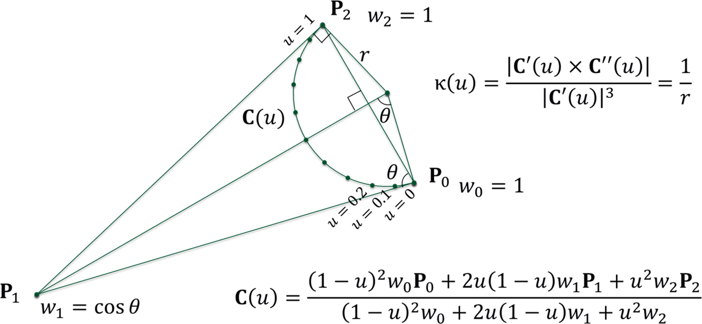
Fig. 3. Circular arc type basic element represented by a parametric curve  ${\bf C}(u)$ with curvature κ(u).
The convex hull property applies. Curvature κ is defined by  $\vert {{\bf C}{\rm^{\prime}} \times {\bf C}^{\rm \prime \prime}} \vert / \vert {{\bf C}^{{\prime}}} \vert ^3$ where ${\bf C}{\rm ^{\prime}}$ and ${\bf C}^{\rm \prime \prime} $ are the first and second derivatives with respect to u. Radius is the reciprocal of curvature and both are constant for a circular arc. The central angle of an arc could be close to π radians in theory but for numerical stability in the computation, it is limited to about 2π/3. An arc with a wider central angle could be represented by a spline with two or three spans. Furthermore, a complete circle could be represented by a rational quadratic periodic Bézier spline with three spans. Straight lines could also be represented as degenerate circular arcs. Straight lines in either representation work equally well in this implementation.
Determination of curve–curve intersections
Point inversion and point projection (Piegl & Tiller, Reference Piegl and Tiller1997, pp. 229–232) are used recursively on two curves to determine the minimum distance between them. If this distance is very small, it indicates an intersection has been found. Multiple seed values are used to ensure both intersections are found if there are two. Virtual intersections beyond the interval 0 ≤ u ≤ 1 are rejected. Given two curves  ${\bf C}(u)$ and ${\bf D}(t)$, and their seed values ${\bf P} = {\bf D}(t_0)$ and ${\bf Q} = {\bf C}(u_0)$, the Newton–Raphson method is applied to a pair of parametric equations.
 $$u_{i + 1} = u_i - \displaystyle{{{\bf C}{\rm ^{\prime}}(u_i) \cdot ({\bf C}(u_i) - {\bf P})} \over {{\bf {C}^{\prime \prime}}(u_i) \cdot ({\bf C}(u_i) - {\bf P}) + {\vert {{\bf C}{\rm^{\prime}}(u_i)} \vert } ^2}}\comma \,$$
 $$t_{i + 1} = t_i - \displaystyle{{{\bf D}{\rm ^{\prime}}(t_i) \cdot ({\bf D}(t_i) - {\bf Q})} \over {{\bf {D}^{\prime \prime}}(t_i) \cdot ({\bf D}(t_i) - {\bf Q}) + {\vert {{\bf D}{\rm^{\prime}}(t_i)} \vert } ^2}}.$$
Iteration continues until both point coincidence and zero cosine are satisfied, unless it is determined that there are no intersections. Two zero tolerances are used, a measure of Euclidean distance ε 1 = 10−8, and a zero cosine measure ε 2 = 10−11. When the base unit of length is a meter, ε 1 denotes that any distance closer than 0.01 µm is considered as coincident. Angle tolerance ε 2 implies that the modeling space is limited to a 1 km cube. No further tolerance analysis is performed. A pragmatic view was taken that there is sufficient precision to support processes like seeing and doing with paper and pencil, product design, and most architectural design purposes. These tolerances are taken from a popular solid modeling kernel, Parasolid. There is no need to differentiate curve–curve intersections from curve–line or line–line intersections.
Transformation matrices
This paper considers an initial shape C and a shape rule A → B. Automatic shape recognition relies on finding a complete list of transformations that satisfy t(A) ≤ C. Each transformation t is represented by a 4 × 4 homogeneous matrix which is defined by two sets of triple registration points (Fig. 4).
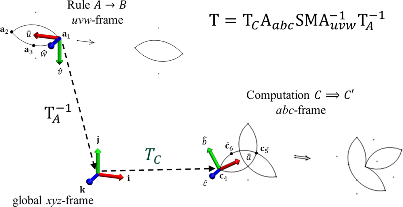
Fig. 4. A transformation t represented by a 4 × 4 homogeneous matrix  ${\bf T}$.
Shape A (and shape B) is defined within a local uvw-frame. Three non-collinear points  ${\bf a}_1\comma \,{\bf a}_2\comma \,{\bf a}_3$ from A are taken at each time. The first point ${\bf a}_1$ is the local origin of shape A. Vector $\overrightarrow {{\bf a}_1{\bf a}_2} $ denotes the u-direction. Vector $\overrightarrow {{\bf a}_1{\bf a}_3} $ is on the uv-plane. Their normalized cross-products are used to derive the orthogonal unit vectors $\hat u\comma \,\hat v\comma \,\hat w$ of their uvw-frames. Each of them is denoted in terms of unit vectors ${\bf i}\comma \,{\bf j}\comma \,{\bf k}$ from the global xyz-frame.
 $$\left\{ {\matrix{ {\hat u = \displaystyle{{\overrightarrow {{\bf a}_1{\bf a}_2}} \over {\vert {\overrightarrow {{\bf a}_1{\bf a}_2}} \vert }}}\hfill \cr {\hat w = \displaystyle{{\hat u \times \overrightarrow {{\bf a}_1{\bf a}_3}} \over {\vert {\hat u \times \overrightarrow {{\bf a}_1{\bf a}_3}} \vert }}} \cr {\hat v = \hat w \times \hat u} \hfill\cr}} \right..$$
 Likewise, shape C is defined in a local abc-frame. Its origin and three orthogonal unit vectors,  $\hat a$, $\hat b$, $\hat c$, are computed from three non-collinear registration points ${\bf c}_4\comma \,{\bf c}_5\comma \,{\bf c}_6$ from C. Translation from the local origin ${\bf a}_1$ of shapes A and B to the global origin is given by ${\bf T}_A^{ - 1} $. Rotation from the local uvw-frame to align with the global xyz-frame is given by ${\bf T}_{uvw}^{ - 1} $. If the mirror of a rule is used, matrix
 $${\bf M} = \left[ {\matrix{ {\matrix{ 1 & 0 \cr 0 & 1 \cr}} & {\matrix{ 0 & 0 \cr 0 & 0 \cr}} \cr {\matrix{ 0 & 0 \cr 0 & 0 \cr}} & {\matrix{ { - 1} & 0 \cr 0 & 1 \cr}} \cr}} \right];$$
otherwise matrix  ${\bf M}$ is an identity matrix. The proportional scaling factor s is used to define a scaling matrix ${\bf S}$, where $\; s = \vert {\overrightarrow {{\bf a}_1{\bf a}_2}} \vert /\vert {\overrightarrow {{\bf c}_4{\bf c}_5}} \vert $. Rotation from the global xyz-frame to align with the local abc-frame is given by ${\bf A}_{abc}$. Translation from the global origin to the local origin of shape C is given by ${\bf T}_C$. Hence, a transformation, t, is represented by the following 4 × 4 homogeneous matrix ${\bf T}$ (Faux & Pratt, Reference Faux and Pratt1979, pp. 70–78).
 $${\bf T} = {\bf T}_C{\bf A}_{abc}{\bf SMA}_{uvw}^{ - 1} {\bf T}_A^{ - 1}. $$
Computational geometry in steps 1 and 4
Step 1 divides an initial shape C into atoms according to matching transformations that satisfy t(A) ≤ C. The input to this step is shape C, which is expected to be in maximal representation. If this condition cannot be ascertained, it is necessary to test and to combine elements if required to ensure all basic elements are maximal to one another (Krishnamurti, Reference Krishnamurti1980). By applying one valid transformation at a time, each basic element is divided into two or three relatively maximal parts or remains unchanged. Each part has the same original carrier curve. The original curve is defined with a parametric variable in the domain [0, 1]. Relatively maximal parts partition this into two or three non-overlapping domains joining end-to-end. Each atom consists of one or more relatively maximal parts. Output to this step is a list of symbolic references, each of which refers to an atom.
Step 4 applies a chosen shape rule under transformation t(A) → t(B). The input to this step is a set grammar with the rule A → B and a chosen transformation t. This results in an intermediate shape C − t(A) in atoms and t(B) in one atom. The shape sum is computed from these two shapes. The resulting shape [C − t(A)] + t(B) is obtained after converting it into a maximal representation using computational geometry techniques such as joining multiple curve spans into a spline and knot insertion (Piegl & Tiller, Reference Piegl and Tiller1997, pp. 141–161). Hence, one shape rule application (Figs. 5b, 9b) of a shape grammar is accomplished. Both steps 1 and 4 are computational geometry operations.
Fig. 5. Triangles grammar (Stiny, Reference Stiny1994).
Shape computation with set grammar in steps 2 and 3
Step 2 generates a lattice (Figs. 8, 12). The input to this step is a set of atoms where each atom is referred to with a symbolic reference and only this symbolic reference is used in this step without any reference to its actual geometry. In this step, shape C is denoted by a set of all atoms, and is the supremum of the lattice.
In step 3, a human user selects one from all valid transformations. There are two possible ways to group and to present all possible transformation to a user. It could be either a list of all possible subshape matches (Figs. 6a, 10a) or a list of visual equivalents of all possible resulting shapes (Figs. 6b, 10b). The output of this step is a chosen transformation that applies to a shape rule. However, the presented shapes are in atomic form and are only visually equivalent to their maximally represented counterparts.

Fig. 6. Different shape computation of the shape grammar of triangles.
Two case studies
Two examples, the triangles grammar (Stiny, Reference Stiny1994) and the trefoil grammar (Jowers & Earl, Reference Jowers and Earl2010), are used to show how steps 2 and 3 are performed in practice.
The triangles grammar
One possible shape rule application (Fig. 5b) of a shape rule (Fig. 5a) is shown. Its U 13 basic elements are straight lines. Five matches (Fig. 6a) produce five different resulting shapes [C − t(A)] + t(B) (Fig. 6b). In fact, each match could be produced from 12 different transformations because of symmetry but, in this grammar, all 12 produce the same resulting shape. In step 2, shape C is decomposed into six atoms (Fig. 7) and a complemented distributive lattice (Fig. 8) is generated that enumerates all possible matches of t(A) and their complements, C − t(A). The triangles lattice (Fig. 8) has a height of 6 and 22 nodes in total.
Fig. 7. Decomposition of the initial shape C of the shape grammar of triangles into six atoms.
Fig. 8. Lattice of the initial shape C of the triangles grammar decomposed by Rule 1.
Because of the symmetries of the left- and right-hand shapes of rule 1, there are multiple transformations that produce the same t(B) but, in general, this is not the case. Here we consider all potential shape rule applications to the same equilateral triangle in the initial shape. Consider rule 2, which has the same left-hand shape as rule 1. Its right-hand shape does not have any symmetry and it is a solid in U 33 (Fig. 13a). The right-hand side of Rule 2 is an extrusion of the right-hand equilateral triangle of rule 1 plus an additional geometry to break the symmetries. Rule 2 could be applied to the initial shape with three different transformations from the front (Fig. 13b). Since the rule operates in a 3D space, three more shape rule applications could be made from the back (Fig. 13c). Since the mirror of a rule is also a valid rule, there are six more potential shape rule applications (Fig. 13d). There are altogether 12 valid transformations since the left-hand shape of rule 2 is identical to that of rule 1. With rule 1, all 12 resulting shapes t(B) are identical. However, with rule 2, all 12 t(B) are different. Hence, all the 12 resulting shapes [C − t(A)] + t(B) are different.
Decomposition of shape C (Fig. 7) in connection with rule 1 is the basis for constructing the lattice (Fig. 8). The way in which this decomposition is made is the same as for the trefoil grammar and described in the next section. In the current implementation, step 3 is carried out by a user who manually selects from the possible rule applications identified in step 2.
Trefoil grammar
A similar sequence is shown for the trefoil grammar (Fig. 9). Its U 13 basic elements are circular arcs. Three matches (Fig. 10a) produce six different resulting shapes [C − t(A)] + t(B) (Fig. 10b). In fact, each match could be produced from eight different transformations. The shape C has six atoms (Fig. 11). The complemented distributive lattice generated in step 2 (Fig. 12) enumerates all possible matches of t(A) and their complements C − t(A). The trefoil lattice (Fig. 12) has a height of 4 and 20 nodes.
Fig. 9. Trefoil grammar.
Fig. 10. Different shape computations of the trefoil grammar.
Fig. 11. Decomposition of the initial shape C of the trefoil grammar into six atoms.
Fig. 12. Lattice of the initial shape C of the trefoil grammar decomposed by rule 3.
The lattice for this grammar differs from the previous one, even though both have six atoms. This is because the left-hand side shapes A of the triangles grammar consist of two atoms in some cases or three atoms in others, whereas, the left-hand side shape A of the trefoil grammar consists of three atoms for each matching t(A). This shows how the generated lattice structure varies according to the initial shape, and the left-hand side of a shape rule.
Similar to rules 1 and 2, the relationship between rules 3 and 4 are used demonstrate the effect of symmetries of the left- and right-hand shapes, or the lack of them. Here we consider all potential shape rule applications to the same leaf in the initial shape. Rule 4 (Fig. 14a) could be applied twice from the front (Fig. 14b) and twice from the back (Fig. 14c). With the mirrored rule, there are four further valid transformations (Fig. 14d). With rule 3, there are eight valid transformations for one leaf of the initial shape and there are two different t(B). However, with rule 4, there are eight different t(B) and, therefore, eight different resulting shapes.
As with the triangles grammar, in the current implementation, step 3 is carried out by a user who manually selects from the possible rule applications identified in step 2.
A note on 2D versus 3D shape rules
Both the triangles grammar and the trefoil grammar were originally defined in U 12 algebra. By translating them into U 13 algebra, we are able to show the effect of symmetries of the left-hand shape A and right-hand shape B. There are more matches in three dimensions that do not exist in two dimensions. Figures 13, 14 show the effect of lack of symmetry of the right-hand shape B. With Rule 1 (Fig. 5a), for every one of the five matched triangles, there is one distinct right-hand shape (Fig. 6b) whereas with rule 2, there are 12 (Fig. 13b–d). With rule 3 (Fig. 9a), for each one of the three matched leaves, there are two distinct right-hand shapes (Fig. 10b) whereas with rule 4, there are eight (Fig. 14b–d).

Fig. 13. Twelve matching transformations t and 12 corresponding resulting shapes t(B) for shape rule 2: A → B.

Fig. 14. Eight matching transformations t and eight corresponding resulting shapes t(B) for shape rule 4: A → B.
From basic elements to relatively maximal parts to atoms
The process of set grammar computation with the triangles grammar and that of the trefoil grammar are similar, but the basic elements used in trefoil grammar are more complex. Details of the trefoil grammar computation are described here as an example. The same general principle of decomposition applies to both grammars.
The initial shape (Fig. 2a) of the trefoil grammar in maximal representation has three basic elements C = {U, T, V} (Fig. 2b). Superimposing each of the three matches of t(A) onto C in turn, each basic element is divided into three relatively maximal parts. Hence, C = {{u 1, u 2, u 3}, {t 4, t 5, t 6}, {v 7, v 8, v 9}} has nine relatively maximal parts (Fig. 2c). The parts of C are relatively maximal to one another but C is not in maximal representation anymore. Each of the three subshape matches can be produced from eight different transformations. Each set of eight transformations produces the same t(A). Some combinations of these relatively maximal parts form partitions. All parts of a partition are either all subshapes of t(A) or C − t(A), but not both and not partially in or out. Each partition of relatively maximal parts is called an atom. The analog of an atom is useful here. An atom could consist of more than one relatively maximal part, but it is the smallest indivisible unit in the context of a set grammar derived from a shape grammar under all possible t(A) matches in an initial shape C. Shape C of this set grammar has six atoms (Fig. 2d), which constitute shape C = {u 2, v 8, t 5, {t 6, v 9}, {u 3, t 4}, {u 1, v 7}}. We can rename these atoms as C = {a, b, c, d, e, f} (Fig. 2d) which correspond to the previous partitions. There are 24 transformations, t 1, t 2, …, t 24, that satisfy t(A) ≤ C. We select three (Fig. 2e–g) transformations that have three different t(A). They are t 3(A) = {b, c, d}, t 7(A) = {a, b, f}, t 11(A) = {a, c, e}.
Among the eight transformations that would produce a t(A) that is the same as t 3(A), four of them would have the same t(B), and the other four have a different t(B). There are altogether six possible t(B) as shown in Figure 10b, which are t 3(B), t 7(B), t 11(B), t 15(B), t 19(B), t 23(B). Among all 24 valid transformations, there are six distinct set grammar computations using symbolic references to relatively maximal parts (Table 2). Three matches of t(A) ≤ C are shown in Figure 10a. The six resulting shapes [C − t(A)] + t(B) are shown in Figure 10b.
Table 2. Shape computation in a set grammar using symbolic references

Relatively maximal parts of C are recombined to form atoms using all matching transformations. These are computed from the algorithm shown below.
ONE partition_of_C ← relatively_maximal_parts_of_C
FOR EACH transformation
basic_elements_of_t(A) ← transformation OF basic_elements_of_A
FOR EACH partition_of_C
set_intersect ← partition_of_C ∩ basic_elements_of_t(A)
set_difference ← partition_of_C \ basic_elements_of_t(A)
THIS partition_of_C ← set_intersect
NEW partition_of_C ← set_difference UNLESS EMPTY SET
END FOR EACH
END FOR EACH
EACH atom_of_C ← EACH partition_of_C
Then, each t(A) is rerepresented using the symbolic references of the atoms of C.
FOR EACH transformation
basic_elements_of_t(A) ← transformation OF basic_elements_of_A
FOR EACH atom_of_C
basic_elements_of_an_atom ← ELEMENTS OF atom_of_C
atoms_of_t(A) ← EMPTY SET
FOREACH basic_elements_of_atom
IF ALL basic_elements_of_an_atom IS IN basic_elements_of_t(A)
atoms_of_t(A) ← atoms_of_t(A) + atom_of_C
END IF
END FOR EACH
END FOR EACH
END FOR EACH
Discussion
Implementation details related to the representation of basic elements, their division into relatively maximal parts, and the use of control vertices to describe circular arcs are considered in the first three parts of this section. The final two sections compare this implementation with that of the quad interpreter (QI) and consider the benefits of using a generalized description of U 13 basic elements.
Representation of basic elements
Two different types of basic element (parametric curve) were used in this implementation: straight line, and circular arc up to a subtending angle of 2π/3. Both are represented by a parametric equation which is defined with its parametric variable for the interval [0,1]. A straight line is a constant speed curve with respect to its parametric variable. A circular arc type basic element is represented by a quadratic rational Bézier curve. If the maximum subtending angle is limited to 2π/3, its speed deviates by 19% at the most. A circular arc type basic element could be degenerated into a straight line type if the middle control vertex is coincident with the line adjoining the first and third vertices, and/or the weight of the second vertex is set to zero. A circular arc with a wider subtending angle is represented by a Bézier spline with two or three spans. In terms of finding intersection(s) of any two basic elements, the type of U 13 basic element is immaterial. Exactly the same routine is used since all of them are in maximal representation and defined when their parametric value is within the interval [0, 1].
Dividing a basic element into its relatively maximal parts
Under transformations and subshape matches, a basic element is divided into a number of relatively maximal parts. With a subshape match under a particular transformation, a breaking point can be found on a basic element (and parametric curve). With repeated application, multiple breaking points can be made on a basic element. Figure 7 shows each of the three outer straight line type basic elements divided into two relatively maximal parts whereas the three inner straight lines remain unchanged. The original straight line basic element is defined with a parametric variable in the interval [0, 1] whereas, the two relatively maximal parts are defined in the intervals of [0, 0.5] and [0.5, 1] using the same carrier curve/line. It is advantageous not to change the carrier curve but simply specifying different ranges of a parametric variable. This is significantly different from previous implementations. It is similar to the use of collinear maximal lines as a descriptor or a carrier line used by Krishnamurti and Earl (Reference Krishnamurti and Earl1992). But instead of spelling out the coordinates of the endpoints of lines/curves, a single value of a parametric variable used. In turn, by applying a parametric value onto curves, the 3D coordinates of the required point can be determined.
Figures 11, 2c shows each of the three circular arcs divided into three relatively maximal parts. The use of parametric curves in this work is essentially the same as that of Jowers and Earl (Reference Jowers and Earl2010). The main difference is that we do not require new control polygons for any new relatively maximal parts; instead, we vary the ranges of the parametric variable on the same carrier line, curve or spline. Figure 2c shows each of the three circular arc type basic elements divided into three relatively maximal parts. The ranges of their parametric variables are [0, 0.41], [0.41, 0.59], and [0.59, 1].
Control vertices of a rational quadratic Bézier curve
A quadratic Bézier curve (Fig. 3) in general has three control vertices,  ${\bf P}_0\comma \,{\bf P}_1\comma \,{\bf P}_2$. In this paper, circular arcs are represented by a special case of a rational quadratic Bézier curve. The middle control vertex lies on the perpendicular divider of the line $\overline {{\bf P}_0{\bf P}_2} $ adjoining the first and last control vertices, where their weights are set to unity, w 0 = w 2 = 1. The weight of the middle vertex is set to a value such that this rational curve is an exact representation of a circular arc, that is, $w_1 = \cos (\pi /2 - \angle {\bf P}_0{\bf P}_1{\bf P}_2/2)$. Degeneration of a circular arc to form a straight line is allowed by positioning the middle vertex to lie on the midpoint of $\overline {{\bf P}_0{\bf P}_2} $ and/or setting the weight of the middle vertex to zero, that is, w 1 = 0. This is effectively degree elevation (Piegl & Tiller, Reference Piegl and Tiller1997, pp. 188–212) that allows algorithms designed for rational quadratic curves to operate correctly on non-rational linear curves.
Comparison between QI and the proposed approach
QI (Jowers & Earl, Reference Jowers and Earl2010) is the most advanced shape grammar implementation that uses curves as basic elements. In this section, we compare and contrast QI and the proposed approach (Table 3), especially by considering the calculation of the intermediate shape C − t(A) and its implications on the ease of implementation. When the subshape relation t(A) ≤ C is satisfied, two ways of embedding could occur between a basic element of t(A) and a corresponding basic element in C. Firstly, if a basic element of t(A) is co-equal to an element of C, it remains unchanged. Secondly, if a basic element of t(A) is a proper subshape of C, it is divided into two or three relatively maximal parts depending exactly how the two basic elements are embedded.
Table 3. Comparison between QI and the proposed approach
When QI divides a basic element into two or three relatively maximal parts, each part is defined by a new control polygon. De Castejljau's algorithm is used to compute the new control vertices. Each relatively maximal part is defined when the parametric variable is within the interval [0, 1]. In this paper, when a basic element is divided into its relatively maximal parts, all parts are represented by the same parametric curve of the original basic element, but they are defined by discrete and complementary intervals, for example, [0, a], [a, b], and [b, 1], where a, b are the parametric values where the basic element splits. There are several implications of these two approaches.
Firstly, in QI a quadratic Bézier curve is represented by a parametric equation,  ${\bf B}_2(t) = t^2{\bf a} + t{\bf b} + {\bf c}$, where ${\bf a}\comma \,{\bf b}\comma \,{\bf c}$ are defined in terms of the control vertices ${\bf b}_0\comma \,{\bf b}_1\comma \,{\bf b}_2$, to represent a curve of a conic section. In this paper, we used the rational form of another parametric equation ${\bf C}(u) = (1 - u)^2{\bf P}_0 + 2u(1 - u){\bf P}_1 + u^2{\bf P}_2$, where ${\bf P}_0\comma \,{\bf P}_1\comma \,{\bf P}_2$ are the control vertices, as an exact representation of a circular arc.
Secondly, in QI, the embedding relation of two basic elements, one from t(A) and the other from C, is determined by intrinsic comparison of curvatures. The curvature of each basic element is represented by an explicit function with four coefficients A, B, C, D for each curve. In turn, these coefficients are defined by non-linear equations in terms of  ${\bf a}\comma \,{\bf b}$ and ultimately ${\bf b}_0\comma \,{\bf b}_1\comma \,{\bf b}_2$. Two curvature functions are related by parameters λ, μ, ν which are defined in terms of coefficients A 1, B 1, C 1, D 1, A 2, B 2, C 2, D 2. In contrast to the proposed approach, the embedding relation is determined by projecting three points from the element of t(A) onto the element of C. If the minimum distances between all three point projections are less than a zero measure ε 1 = 10−8, the embedding relation is deemed to be satisfied With one or both ends of the element from t(A) acting as the splitting points for the element from C. This could result in one, two, or three relatively maximal parts of C. The proposed approach is simpler in terms of dividing a basic element into its part for later use. The original basic elements and its relatively maximal parts share the same carrier curves but with different parameter ranges.
Thirdly, QI considers Bézier curves as distinct from straight lines, so degeneration of a Bézier curve into a straight is not permitted. For this reason, curve–curve, curve–line, and line–line intersections are considered as three different cases. Numerical stability when a curvature is close to zero was not investigated but it is likely to be necessary to impose a minimum curvature limit to avoid division by numbers close to zero. As a result, two different algorithms are required: one for Bézier curves and the other one for straight lines. In this paper, a degenerate straight line can be represented as a Bézier curve (as outlined in the subsection “Control vertices of a rational quadratic Bézier curve”). With the proposed approach, whether a basic element is a true curve or a straight line is immaterial. They can be dealt with by the same algorithm equally well and, whatever the actual geometry, only one algorithm is necessary for intersections between any two basic elements of any type. Fourthly, for a particular embedding relation, QI is required to determine, which one among all eight possible ways, one basic element is embedded within another one. The ordering of the parametric variables of each curve is important. In this paper, a coincidence test of three points on a curve is needed for testing the embedding relation. The order of testing each of the three points is immaterial. The direction of the parametric variable is immaterial too.
Finally, the most important aspect of the proposed implementation is the use of atoms. QI repeats the above operation for each matching transformation while in this work, a set of atoms and shapes derived from them form a lattice. Each matching t(A), among other shapes, is already a node in this lattice.
Benefits of a generalized description of U13 basic elements
In concluding the discussion of implementations for general (Bézier) curves and circular arcs, we note that the example of the trefoil grammar is a special case for the application of the general curve grammar. However, the circular arc implementation concentrates on addressing the specific geometrical elements arising in the trefoil configurations. In design applications of shape grammars, there is a tension between creating tools specific to geometrical elements of interest and more general tools applicable across a wider range of geometric elements. This paper has demonstrated that limiting geometrical elements can focus attention on the details of where and how emergence occurs as well as the necessary shape computations to implement it in a design context. In particular, the paper indicates that a separation between geometric calculation and shape computation assists the development of usable and extensible tools for shape grammar implementation.
Conclusions and future work
The ideas presented in this paper came from research on the use of hypercube lattices to support the configuration of bills of materials (BOMs) in engineering product development processes (Kodama et al., Reference Kodama, Kunii and Seki2016). Important benefits of using lattices for the configuration of BOMs are that they provide: (i) a self-consistent computational space within which BoMs can be manipulated and (ii) connectivity to the source design description that allows users to move back and forth between BOMs and other forms of design description. The type of relationship between parts in a BOM (part–whole relationships) is the same as that between shapes and sub-shapes in shape grammars. This led to us exploring a potential application to shape grammar implementation.
The significance of the proposed approach for software implementation of shape grammars is that computational geometry and shape computation are decoupled. A temporary set grammar is generated using an initial shape and a shape rule and represented as a complemented distributive lattice. All occurrences of the left-hand side of the rule in the initial shape are nodes in the lattice. For this reason, shape computation can be performed without considering the actual geometries of the shapes involved. Decoupling the geometry and grammar has resulted in two desirable outcomes. Firstly, shape algebra operations – shape difference and shape sum – are equivalent to complements and joins of nodes in the lattice. This allows the results of shape algebra operations to be derived from the lattice rather than calculated. Secondly, an extension to include more types of shape element will not change the shape computational aspect of a shape grammar implementation. A new set grammar is generated for each rule application in a given shape computation process.
A medium-term objective of the presented approach is to allow shape grammar to be used in domains that require freeform geometries, for example, consumer products. In a wider context, shape emergence and calculation with shapes have been studied by scholars from different disciplines (Wittgenstein, Reference Wittgenstein1956; Stiny, Reference Stiny1982; Tversky, Reference Tversky, Kutz, Bhatt, Borgo and Santos2013). Minsky's (Reference Minsky1986, p. 209) enquiry on visual ambiguity and Stiny's (Reference Stiny2006; p. 136) different views on the Apple Macintosh logo examples are examples of multiple interpretations. This research brings closer software tools that realize the potential of calculation with shapes for theoretical studies as well as laying a foundation for practical tools in various spatial design contexts.
Acknowledgments
This research is supported by the UK Engineering and Physical Sciences Research Council (EPSRC), under grant number EP/N005694/1, “Embedding design structures in engineering information”. We are also grateful to the anonymous reviewers for their constructive comments.
Hau Hing Chau is a teaching fellow in the School of Mechanical Engineering at the University of Leeds. He obtained his PhD in 2002 from the University of Leeds on the preservation of brand identity in engineering design using a grammatical approach. Since then, his research has focused on shape computation and the implementation of 3D shape grammar-based design systems for use in the consumer product development processes.
Alison McKay is a Professor of Design Systems in the School of Mechanical Engineering at the University of Leeds. Her research focus on three kinds of design system: shape computation and information systems used to create designs and develop products, and the socio-technical systems within which designers work and in which their designs are used. Her research is positioned within the context of stage-gate processes that typify current industry practice and aims to facilitate improved modes of working through the exploitation of digital technology and to establish design methods, and tools to support systematic evaluation of design alternatives at decision gates.
Christopher Earl has been a Professor of Engineering Design at the Open University since 2000. He obtained his PhD in design from the Open University and works closely with a wide range of research groups in design and shape computation worldwide. Prior to 2000, he held positions at Newcastle University, affiliated with the Engineering Design Centre in the Faculty of Engineering, where his research concentrated on the design and manufacture processes for large, complex, engineering to order products, particularly their planning and scheduling under uncertainty. Dr Earl's main research interests are in generative design, models of design processes, and comparisons across design domains.
Amar Kumar Behera holds BTech, MTech, and minor degrees from Indian Institute of Technology, Kharagpur; MS from the University of Illinois, Urbana-Champaign; and PhD from the Katholieke Universiteit Leuven. He joined Mphasis an HP company in 2008 and later worked as an Assistant Professor at Birla Institute of Technology and Science, Pilani, and a research fellow at the University of Nottingham. Since 2015, he has been with the University of Leeds, where he is a research fellow. His main areas of research interest are digital manufacturing and design informatics. Dr Behera is an associate fellow of the UK Higher Education Academy and has published 35 peer-reviewed articles.
Alan de Pennington OBE PhD held the Chair of Computer Aided Engineering at the University of Leeds from 1984 to 2005. When he retired, an Emeritus Professorship was conferred on him. His research interests include modeling in the design process, product data engineering, shape grammars and shape computation, engineering enterprise integration, and business processes. He was the Director of the Keyworth Institute from 1994 to 2004, which was a multidisciplinary research institute which enabled collaboration between the Business School and Engineering. This led to ongoing research in supply chain innovation.


 Open access