


Impact Statement
Environmental data often contain many candidate covariates and unbalanced response variables. For example, when modeling species distributions of rare species, nondetections are often considerably more common than detections. While random forest is robust to situations with many covariates compared to data points, inference and prediction can be negatively affected by data imbalance, especially at the medium to small sample sizes common in environmental data. Using area under the curve (AUC) to calculate variable importances and as a criterion in variable selection improved the identification of true predictor variables when data were unbalanced. Therefore, at least when sample sizes are relatively small, we recommend the use of AUC in variable ranking and selection with random forest to improve inference and prediction.
1. Introduction
Random forest is a machine learning algorithm (Breiman, Reference Breiman2001) used for a variety of purposes, for example in genetics (Díaz-Uriarte and de Andrés, Reference Díaz-Uriarte and de Andrés2006), to predict the occurrence of storms (Ruiz-Gazen and Villa, Reference Ruiz-Gazen and Villa2007), biomass (Adam et al., Reference Adam, Mutanga, Abdel-Rahman and Ismail2014), wetland inundation (Karimi et al., Reference Karimi, Saintilan, Wen and Valavi2019), the distribution of species (Garzón et al., Reference Garzón, Blazek, Neteler, de Dios, Ollero and Furlanello2006; Bradter et al., Reference Bradter, Kunin, Altringham, Thom and Benton2013; Robinson et al., Reference Robinson, Ruiz-Gutierrez and Fink2018; Ryo et al., Reference Ryo, Angelov, Mammola, Kass, Benito and Hartig2021), or to map vegetation from remotely sensed data (Sesnie et al., Reference Sesnie, Gessler, Finegan and Thessler2008; Bradter et al., Reference Bradter, Thom, Altringham, Kunin and Benton2011; O’Connell et al., Reference O’Connell, Bradter and Benton2015; Barrett et al., Reference Barrett, Raab, Cawkwell and Green2016; Bradter et al., Reference Bradter, O’Connell, Kunin, Boffey, Ellis and Benton2020). Advantages of random forest include its often high classification accuracies (Garzón et al., Reference Garzón, Blazek, Neteler, de Dios, Ollero and Furlanello2006; Prasad et al., Reference Prasad, Iverson and Liaw2006; Cutler et al., Reference Cutler, Edwards, Beard, Cutler, Hess, Gibson and Lawler2007; Strobl et al., Reference Strobl, Malley and Tutz2009; Sluiter and Pebesma, Reference Sluiter and Pebesma2010) and its robustness to situations with many covariates relative to data points (Grömping, Reference Grömping2009). However, when one or several classes are much less prevalent than another class (unbalanced data), ranking and selection of covariates and classification with random forest can be problematic (Chen et al., Reference Chen, Liaw and Breiman2004; Lin and Chen, Reference Lin and Chen2012; Janitza et al., Reference Janitza, Strobl and Boulesteix2013).
Random forests use bagging and combine many regression or classification trees in an ensemble (Breiman, Reference Breiman2001). Each of the many trees in the forest is grown on a random selection, typically two-third, of the data. Additional randomization is introduced by restricting the available predictors at each node split to a random selection. This randomness produces a diverse ensemble of trees and can result in more accurate results (Breiman, Reference Breiman2001; Liaw and Wiener, Reference Liaw and Wiener2002; Strobl et al., Reference Strobl, Malley and Tutz2009). Each tree is used to predict the data not used in the construction of the tree, the out-of-bag (OOB) data. For each datapoint, the majority vote of all predictions is used to produce an average prediction in classification. The OOB error is the proportion of datapoints for which this average prediction is not the same as the true class (Liaw and Wiener, Reference Liaw and Wiener2002). For inference with random forest, variable importance measures can be calculated. The permutation importance is calculated by randomly permuting each covariate in turn to destroy a potential association with the response variable. It is calculated as the difference in OOB error from the model with the permuted covariate compared to the OOB error from the model without permutations (Strobl et al., Reference Strobl, Boulesteix, Zeileis and Hothorn2007). For a detailed description of random forest see, for example, Breiman (Reference Breiman2001), Liaw and Wiener (Reference Liaw and Wiener2002), Grömping (Reference Grömping2009), and Strobl et al. (Reference Strobl, Malley and Tutz2009).
Unbalanced data are widespread in ecology and environmental science and can affect variable importance measures and the accuracy of classification results. For example, in remote sensing of vegetation, the rarer vegetation classes tend to be much less prevalent in the data (Bradter et al., Reference Bradter, O’Connell, Kunin, Boffey, Ellis and Benton2020). Species distributions are often mapped using reported detections and non-detections of the species at sample locations collected by survey schemes (Franklin, Reference Franklin2009). For rarer species, it is common to have considerably more non-detections than detections. The majority class (e.g., non-detections) tends to be predicted with a higher accuracy than the minority class (e.g., detections) in random forest (Chen et al., Reference Chen, Liaw and Breiman2004; Lin and Chen, Reference Lin and Chen2012) and permutation importances are biased at higher imbalance levels (Janitza et al., Reference Janitza, Strobl and Boulesteix2013). This can be problematic, for example for conservation and land management, because targeted conservation measures depend on predicting the occurrence of the rare species or vegetation types accurately and on accurate inference of the processes that lead to the observed pattern.
Several adaptations have been proposed to improve the performance of random forest with unbalanced data. However, the adaptations have frequently been evaluated regarding their ability to discriminate between classes and it remains unclear how variable importance measures and therefore the ranking and selection of covariates are affected. Adaptations to improve the performance with unbalanced data include (a) resampling of data to improve class balance, (b) applying weights, (c) applying a tree-splitting criterion that is robust to data imbalance, and (d) changing the threshold for the assignment of predicted classes. Resampling strategies to improve class balance include to sample only a proportion of the data randomly from the majority class for each classification tree in the ensemble (downsampling) or to oversample the minority class (balanced random forest; Chen et al., Reference Chen, Liaw and Breiman2004; Liu et al., Reference Liu, Chawla, Harper, Shriberg and Stolcke2006; Xu-Ying et al., Reference Xu-Ying, Jianxin and Zhi-Hua2009; Lin and Chen, Reference Lin and Chen2012). Both downsampling and upsampling improved the discrimination between unbalanced classes compared to not applying a resampling strategy (Chen et al., Reference Chen, Liaw and Breiman2004). Downsampling outperformed upsampling, but may result in loss of information (Chen et al., Reference Chen, Liaw and Breiman2004; Liu et al., Reference Liu, Chawla, Harper, Shriberg and Stolcke2006). Applying weights at node splits and in majority voting has improved the discrimination of classes when data were imbalanced (Chen et al., Reference Chen, Liaw and Breiman2004; Min et al., Reference Min, Jing, Xiaoqing, Molei, Guolong, Jing and Gangmin2018). In contrast to the tree splitting criteria Gini index and Gain Ratio, the Hellinger distance is not biased toward the majority class and the discrimination between classes can improve when the Hellinger distance is used (Cieslak et al., Reference Cieslak, Hoens, Chawla and Kegelmeyer2012; Aler et al., Reference Aler, Valls and Boström2020). Discrimination between unbalanced classes was also improved when the threshold used to distinguish between classes was optimized (Dahinden, Reference Dahinden, Guyon, Cawley, Dror and Saffari2011; Freeman et al., Reference Freeman, Moisen and Frescino2012). Studies that evaluated several of the adaptations against each other, reported contrasting results. Robinson et al. (Reference Robinson, Ruiz-Gutierrez, Fink, Meese, Holyoak and Cooch2018) used spatially biased and imbalanced data consisting of detection and nondetection data of a bird species. After first reducing the spatial bias in the majority class by filtering data based on location, they found that random forest without adjustment for unbalanced data (default random forest henceforth), weighted random forest, balanced random forest, and a more sophisticated resampling strategy, oversampling using synthetic samples (SMOTE), discriminated accurately between detections and nondetections. However, their sample size was large and despite class imbalance, the number of cases of the minority class was more than 1,000. With smaller sample sizes, Chen et al. (Reference Chen, Liaw and Breiman2004) found little difference between balanced and weighted random forests, but both discriminated better between classes than the default random forest. On presence-background data for 225 species with varying sample size, downsampled random forests and versions that combined the Hellinger splitting criterium with shallower trees were better able to discriminate between classes compared to the default random forest or weighted random forest (Valavi et al., Reference Valavi, Elith, Lahoz-Monfort and Guillera-Arroita2021a). The same study also evaluated random forest based on regression trees applied to binary data. We do not consider this version further as it was among the poorer performers, and because binary response variables are not a good fit for a method designed for continuous response variables. Downsampled random forests were also among the algorithms with the highest discrimination for unbalanced classes when compared to methods other than random forest (Valavi et al., Reference Valavi, Guillera-Arroita, Lahoz-Monfort and Elith2021b).
Adaptations to improve variable ranking or selection with unbalanced data are based on the AUC (area under the receiver operating curve), which is insensitive to unbalanced data (Fawcett, Reference Fawcett2006). AUC has been used for the calculation of permutation importances (Janitza et al., Reference Janitza, Strobl and Boulesteix2013), thus affecting the order in which covariates will be ranked for variable selection. AUC has also been used as a criterion in a backward variable selection, however, the ranking of covariates was based on the default version of random forest (Urrea and Calle, Reference Urrea and Calle2012).
The aim of our study was to evaluate the influence of alternative versions of random forest for unbalanced data on variable ranking and variable selection. Using simulated data, we evaluated (a) how highly true covariates were ranked by alternative random forest versions based on variable importances and (b) how well alternative random forest versions were able to identify true covariates out of a large number of covariates despite data imbalance. Subsequently, we present three case studies from the field of species distribution modeling using data with a varying degree of imbalance. We based our study on small to medium sample sizes with imbalance levels of 20% and higher and with weak, medium, and strong associations between the response variables and covariates. Under these conditions, the biases due to unbalanced data are most evident. The performance of variable importances and class discrimination typically declines with increasing class overlap, increasing imbalance level, and decreasing sample size (Lin and Chen, Reference Lin and Chen2012; Janitza et al., Reference Janitza, Strobl and Boulesteix2013). The default random forest produces good discrimination between classes when class distributions are well separated regardless of the class imbalance (Lin and Chen, Reference Lin and Chen2012; Valavi et al., Reference Valavi, Elith, Lahoz-Monfort and Guillera-Arroita2021a).
2. Methods
Our simulations and case studies were based on data sets with many covariates relative to data points. An advantage of random forest is its robustness to situations with many covariates to data points. Consequently, it is particularly valuable to include such data sets in evaluations.
2.1. Simulation study
Using simulated data, we compared how alternative random forest approaches ranked and were able to identify true covariates despite data imbalance. First, we generated 1,080 simulated data sets varying in size, imbalance level, number of true variables, their effect sizes, and the strength of multicollinearity between true and noise variables (Figure 1a,b). Based on 121 real-world environmental covariates, we generated simulated binary data. We named the minority class presences and the majority class absences, thus simulating data frequently used in the field of species distribution modeling (Franklin, Reference Franklin2009). From the 121 covariates, we chose covariates with either low or high multicollinearity to other covariates as true variables. To estimate multicollinearity, we calculated variance inflation factors (VIFs, Zuur et al., Reference Zuur, Ieno, Walker, Saveliev and Smith2009). The simulated occurrences were generated by drawing from the Bernoulli distribution with probability p, the probability of the simulated occurrence being a presence. p was calculated as the inverse logit of the linear predictor α + β 1 × x 1 + … βn × xn, where x 1-n were either one, two, or four true variables with low VIFs or one, two, or four true variables with high VIFs. For each of the six combinations of true variables, we chose regression coefficients β 1-n , that represented weak (β = 0.4), medium (β = 0.9), or strong (β = 1.4) effects, generating 18 simulated responses in total (Figure 1a). The true variables were standardized to a mean of 0 and a standard deviation of 1. Next, we randomly sampled to create 60 data sets from each of the simulated responses (Figure 1b). The data sets varied in sample size (300, 200, 100 absences) and the level of imbalance (20, 15, 10, 5% presences). For each of the 12 combinations of sample size with imbalance level, we randomly sampled five times, generating 1,080 simulated data sets (Figure 1b: 18 simulated responses × 3 sample sizes × 4 imbalance levels × 5 random samples = 1,080).
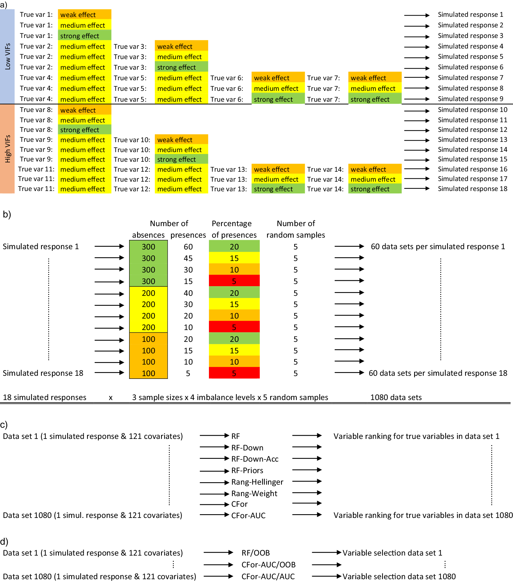
Figure 1. Conceptual diagram of the simulation study: (a) Out of a set of 121 environmental covariates, 14 variables were selected as true variables (true var). Seven of the 14 variables had low variance inflation factors (VIFs) indicating low multicollinearity with other covariates and the other seven variables had high variance inflation factors. True variables were standardized to a mean of 0 and a standard deviation of 1. Eighteen binary, simulated response variables were created based on weak (ß = 0.4), medium (ß = 0.9), and strong (ß = 1.4) effect sizes for true variables and either one, two, or four true variables with either low or high VIFs. (b) From each simulated response variable consisting of presences and absences, 60 datasets were created differing in the sample size (300, 200, or 100 absences) and the imbalance level (20, 15, 10, or 5% presences). Presences and absences were randomly drawn five times for each of the 12 combinations of sample size with imbalance level. In total, 1,080 data sets were created (18 simulated responses × 3 sample sizes × 4 imbalance levels × 5 random samples). (c) For each of the 1,080 datasets consisting of simulated presences and absences and the corresponding 121 environmental covariates, variable importances were calculated for each of the 121 covariates using eight alternative random forest versions: four random forest versions were implemented with R package randomForest (RF, RF-Down, RF-Down-Acc, RF-Priors), two versions were implemented with R package ranger (Rang-Hellinger, Rang-Weight) and two versions with R package party (CFor, CFor-AUC): (1) default RF (RF), (2) the majority class downsampled to the size of the minority class (RF-Down), (3) the majority class downsampled to 64% of the size of the minority class (RF-Down-Acc), (4) weights as class priors (RF-Priors), (5) Hellinger distance as splitting criterion (Rang-Hellinger), (6) weights applied to the splitting rule and majority vote (Rang-Weight), (7) random forest based on conditional inference trees (CFor), (8) random forest based on conditional inference trees with AUC permutation importance (CFor-AUC). After the calculation of variable importances, the covariates were ranked from the covariate with the highest importance to the covariate with the lowest importance and the ranks for true variables were extracted. (d) For each of the 1,080 datasets we carried out variable selection using three alternative versions: (1) Variable ranking based on permutation importances from the default RF, followed by a forward selection with the Out-of-Bag error as selection criterion (RF/OOB), (2) Variable ranking based on AUC permutation importance and forests with conditional inference trees, followed by a forward selection with the Out-of-Bag error as selection criterion (CFor-AUC/OOB), and (3) Variable ranking based on AUC permutation importance and forests with conditional inference trees, followed by a forward selection with the AUC as selection criterion (CFor-AUC/AUC).
2.2. Variable ranking
For each of the 1,080 data sets, we evaluated how highly the true predictors were ranked in comparison to the other covariates by eight alternative algorithm versions (Figure 1c). Four random forest versions were implemented with the R package “randomForest” (Liaw and Wiener, Reference Liaw and Wiener2002). This function implements the original programme by Breiman and Cutler (Liaw and Wiener, Reference Liaw and Wiener2002) and forests are based on CART trees (Breiman, Reference Breiman2001; Strobl et al., Reference Strobl, Malley and Tutz2009). CART trees use the Gini split criterion, which measures the decrease in node impurity, to select the predictor for a node split. Subset sampling for individual trees is with replacement by default (Liaw and Wiener, Reference Liaw and Wiener2002). Two random forest versions were implemented with the R package “ranger,” a fast implementation of random forests (Wright and Ziegler, Reference Wright and Ziegler2017). Two versions were implemented with function cforest from R package “party” (Strobl et al., Reference Strobl, Boulesteix, Zeileis and Hothorn2007; Strobl et al. Reference Strobl, Boulesteix, Kneib, Augustin and Zeileis2008). Random forest with cforest are based on conditional inference trees with predictors for node split selected based on a conditional inference independence test (Strobl et al., Reference Strobl, Boulesteix, Zeileis and Hothorn2007). Variable importances based on cforest optionally allow for the calculation of a conditional version of variable importances (Strobl et al., Reference Strobl, Boulesteix, Kneib, Augustin and Zeileis2008). Although this may be suitable for our data, which contained correlated predictor variables, we did not use it to avoid confounding our comparisons with the previous six algorithm versions. The following eight versions were evaluated:
-
1. RF: Random forest with no adjustment for unbalanced data: function randomForest in package randomForest.
-
2. RF-Down: For each tree in the ensemble, we randomly deselected data from the majority class to match the size of the minority class using option sampsize in function randomForest.
-
3. RF-Down-Acc: Downsampling the majority class to the size of the minority class does not necessarily result in the best performance (Ruiz-Gazen and Villa, Reference Ruiz-Gazen and Villa2007). We downsampled the majority class to 64% of the size of the minority class, which had produced good error rates for the minority class on preliminary simulated data.
-
4. RF-Priors: We provided priors for the classes using the argument classwt of function randomForest (package randomForest). We used the proportion of the absences in the whole data set as the prior for the absence class, and the proportion of presences as the prior for the presence class. To explore the variability in output due to variation in priors, we additionally reversed the order and supplied the proportion of presences as the prior for the absence class and the proportion of absences as the prior for the presence class.
-
5. Rang-Hellinger: We used the Hellinger distance as the splitting rule in function ranger of package ranger.
-
6. Rang-Weight: We used the argument class.weights of function ranger to apply weights for the classes in the splitting rule and in the majority voting. We used the proportion of the absences in the whole data set as the weight for the presence class, and the proportion of presences as the weight for the absence class. To explore the variability in output due to variation in weights, we additionally reversed the order and supplied the proportion of presences as the weight for the presence class and the proportion of absences as the weight for the absence class.
-
7. CFor: We applied random forest based on conditional inference trees with function cforest in package party.
-
8. CFor-AUC: We calculated AUC permutation importance using function varImpAUC in package “varImp” (Probst, Reference Probst2020) in conjunction with function cforest from package party. Function varImpAUC uses AUC instead of OOB in the calculation of permutation importance (Janitza et al., Reference Janitza, Strobl and Boulesteix2013). The permutation importance is calculated as the difference in AUC before and after permutation of each covariate in turn. Permutation importances are therefore expected to be more insensitive to the imbalance level.
For the tuning parameters of random forest, ntree (the number of trees in a forest) and mtry (the number of variables tried at each node split), we used ntree = 2,000 and mtry = p/2 following Genuer et al. (Reference Genuer, Poggi and Tuleau-Malot2010), where p is the number of predictors. Higher ntree settings result in less variability and more stable variable importances and OOB error (Liaw and Wiener, Reference Liaw and Wiener2002; Díaz-Uriarte and de Andrés, Reference Díaz-Uriarte and de Andrés2006; Genuer et al., Reference Genuer, Poggi and Tuleau-Malot2010). The default value in the R package random forest is ntree = 500 (Liaw and Wiener, Reference Liaw and Wiener2002). With higher mtry values, the permutation importance becomes more conditional; with lower mtry values the permutation importance becomes more marginal (Strobl et al., Reference Strobl, Boulesteix, Kneib, Augustin and Zeileis2008; Grömping, Reference Grömping2009). The default value for classification in the R package random forest is mtry = $ \surd p $
(Liaw and Wiener, Reference Liaw and Wiener2002). For each of the 1,080 test sets and each of the eight algorithms, we repeated the calculation of variable importance measures 10 times. We ranked all 121 covariates based on the average variable importances from the 10 repetitions.
$ \surd p $
(Liaw and Wiener, Reference Liaw and Wiener2002). For each of the 1,080 test sets and each of the eight algorithms, we repeated the calculation of variable importance measures 10 times. We ranked all 121 covariates based on the average variable importances from the 10 repetitions.
2.3. Variable selection
We evaluated how well variable selection identified true predictors out of all 121 covariates for three algorithm versions. We implemented the variable selection approach of Genuer et al. (Reference Genuer, Poggi and Tuleau-Malot2010), which consists of a forward selection of variables ranked by their variable importances resulting in a subset of important variables inclusive of some redundant variables. Optionally, the redundant variables can be reduced in an additional step, which we did not implement. The variable selection strategy has been described as a prediction-oriented strategy accepting a higher risk of false negatives, or important covariates that are not in the final selection set (Genuer et al., Reference Genuer, Poggi and Tuleau-Malot2015). The variable selection consisted of the following steps for the default version without adjustments to account for unbalanced data: First, all covariates were ranked by their permutation importance, averaged over 50 repetitions. Second, we calculated OOB error for the model with the highest ranked covariate, averaged over 25 repetitions for each set. We added the second highest ranked covariate, recalculated OOB error and repeated this procedure until all covariates were included. Third, we identified the model with the lowest mean OOB error and added its standard deviation. Then we selected the smallest (fewest covariates) model with an OOB error less than this value. We used the tuning parameters suggested by Genuer et al. (Reference Genuer, Poggi and Tuleau-Malot2010): for the calculation of variable importances, we used ntree = 2,000 and mtry = p/2, where p equals the number of covariates and for the calculation of OOB error we used the default ntree and mtry values of function randomForest. To increase computational efficiency we also followed their recommendation for initial removal of the lowest ranked covariates, based on high standard deviations of permutation importances relative to small mean permutation importance per covariate. For full details of the variable selection strategy, see Genuer et al. (Reference Genuer, Poggi and Tuleau-Malot2010).
We evaluated the following three approaches (Figure 1d):
-
1. RF/OOB: Permutation importances were calculated with the default RF.
-
2. CFor-AUC/OOB: AUC permutation importances were calculated based on the cforest implementation.
-
3. CFor-AUC/AUC: AUC permutation importances were calculated based on the cforest implementation of random forest. Instead of using OOB as the selection criterium in the forward selection, AUC was used. In other words, instead of calculating OOB for each nested model, we calculated AUC. Then, analogue to the selection method based on OOB, we identified the model with the highest mean AUC, subtracted its standard deviation from the mean AUC value, then selected the smallest model with a mean AUC larger than this value as the final model (Figure 2).

Figure 2. Example of model selection using AUC. First, AUC is calculated for all nested models using several repetitions for each nested model. The black curve shows the mean AUC over all repetitions with the gray polygon showing the mean ± standard deviation. Then, the model (vertical black line) with the highest mean AUC (dashed horizontal black line) is identified. The AUC value corresponding to mean–standard deviation for this model (dotted horizontal black line) serves as a threshold accounting for the variation between repetitions. The selected model is the smallest (lowest number of covariates) model with a mean AUC at or above the threshold value (blue lines).
For each selected model, we assessed how well true predictors were identified out of all 121 covariates using sensitivity and specificity. Sensitivity is higher the more true predictors are correctly identified (true positives) and is calculated as:
 $$ \frac{\mathrm{true}\ \mathrm{positives}}{\mathrm{true}\ \mathrm{positives}+\mathrm{false}\ \mathrm{negatives}}, $$
where false negatives are true predictors that were not selected. Specificity is higher the more covariates which are not the true predictors are identified as such (true negatives) and was calculated as:
 $$ \frac{\mathrm{true}\ \mathrm{negatives}}{\mathrm{false}\ \mathrm{positives}+\mathrm{true}\ \mathrm{negatives}}, $$
where false positives are covariates falsely identified as true predictors (Lin and Chen, Reference Lin and Chen2012).
2.4. Case studies
We present studies from the field of species distribution modeling as case studies. Species occurrence data from sample sites are modeled as a function of environmental information in species distribution models. Subsequently, maps of the occurrence of the species can be produced based on the species-environment associations established in the models (Franklin, Reference Franklin2009). Species distribution modelers are often encouraged to carefully select suitable covariates based on ecological knowledge of the species to avoid spurious associations. However, the ecology of many species is poorly studied and understood (Dormann et al., Reference Dormann, Schymanski, Cabral, Chuine, Graham, Hartig, Kearney, Morin, Römermann, Schröder and Singer2012, Urban et al., Reference Urban, Bocedi, Hendry, Mihoub, Pe’er, Singer, Bridle, Crozier, De Meester, Godsoe, Gonzalez, Hellmann, Holt, Huth, Johst, Krug, Leadley, Palmer, Pantel, Schmitz, Zollner and Travis2016), which carries the risk that important processes are inadvertently omitted or misspecified in models. A key consideration in ecology is that each ecological process has an appropriate spatial scale and that appropriate spatial scales are dependent on the organism under consideration (Wiens, Reference Wiens1976; Addicott et al., Reference Addicott, Aho, Antolin, Padilla, Richardson and Soluk1987). This scale of effect is the scale at which the association between a species occurrence and an environmental covariate is strongest (Jackson and Fahrig, Reference Jackson and Fahrig2012). Another key consideration is that ecological processes can act at multiple spatial scales and influence species at individual, group, or population level (Johnson, Reference Johnson1980; Wiens, Reference Wiens1989; Levin, Reference Levin1992; Cunningham and Johnson, Reference Cunningham and Johnson2006; McGarigal et al., Reference McGarigal, Wan, Zeller, Timm and Cushman2016). A covariate influencing a species’ distribution at one scale (e.g., surface water availability within 500 m of a species’ nest site) may exert a different or no influence at a different scale (e.g., within 10 km; Wiens, Reference Wiens1989, Hamer and Hill, Reference Hamer and Hill2000). Including covariates at appropriate spatial scales in ecological models is therefore important. However, if the spatial process scales are unknown, appropriate spatial scales of covariates have to be selected empirically out of a potentially large pool of covariate × scale combinations. Random forest is a candidate algorithm for such problems due to its ability to assess species-environment associations with all covariate × scale combinations simultaneously in one model (Bradter et al., Reference Bradter, Kunin, Altringham, Thom and Benton2013). Such models may generate new hypotheses about the ecological processes determining the distribution of species.
2.5. Study species and data collection
As case studies, we used the wader species (shorebirds in North America) Northern lapwing (Vannellus vanellus), common snipe (Gallinago gallinago), and common redshank (Tringa totanus). We analyzed and mapped their distribution in a part of the Yorkshire Dales, an upland area of the UK. Habitat selection of the three species is well-studied, particularly at finer spatial scales (e.g., Baines, Reference Baines1990; Green et al., Reference Green, Hirons and Cresswell1990; O’Brien, Reference O’Brien2002; Taylor and Grant, Reference Taylor and Grant2004; Smart et al., Reference Smart, Gill, Sutherland and Watkinson2006; Sharps et al., Reference Sharps, Garbutt, Hiddink, Smart and Skov2016). Therefore, species-environment relationships suggested by our models can be assessed against existing knowledge on the species ecology, while at larger spatial scales, there is potential for the generation of new hypotheses. Specifically, at the territory level, all three species are known to be associated with wet conditions (Green et al., Reference Green, Hirons and Cresswell1990; O’Brien, Reference O’Brien2002; Smart et al., Reference Smart, Gill, Sutherland and Watkinson2006). Northern lapwing is also known to preferred gentle over steep slopes and to avoid improved pastures (Henderson et al., Reference Henderson, Wilson, Steele and Vickery2002; Taylor and Grant, Reference Taylor and Grant2004). Northern lapwing is listed as globally near threatened (IUCN, 2022). In the UK, Northern lapwing is listed as red, and common snipe and common redshank as amber conservation status (Woodward et al., Reference Woodward, Massimino, Hammond, Barber, Barimore, Harris, Leech, Noble, Walker, Baillie and Robinson2020). Managing these and other declining species is a major concern to many land managers.
We surveyed Northern lapwing, common redshank and common snipe in 244 observation units (each ca. 300 × 500 m) in the Yorkshire Dales, UK (Supplementary Figure S1). With observation units of this size we aimed to approximate the reported sizes of core areas used during the breeding season (home ranges henceforth): common redshank chicks were found up to 180 ± 68 m from their nests in salt marshes in Germany (Thyen et al., Reference Thyen, Exo, Cervencl, Esser and Oberdiek2008); Northern lapwing chicks up to 202 m (61–386 m) from nests in Swedish farmland (Johansson and Blomqvist, Reference Johansson and Blomqvist1996) and incubating female common snipe foraged 17–390 m from their nests in lowland sites of the UK (Green et al., Reference Green, Hirons and Cresswell1990). We surveyed the observation units from 61 transects (each 2 km long) to minimize traveling time between observation units, where each transect dissected four contiguous observation units. Surveys targeted elevations below 500 m and were carried out during the 2008 breeding season. To reduce the risk of recording false absences each transect was surveyed three times between April 2 and July 1. This covered much of the incubation and chick-rearing periods of the species (Robinson, Reference Robinson2017). Imperfect detection of species can for example be accounted for in occupancy models (MacKenzie et al., Reference MacKenzie, Nichols, Hines, Knutson and Franklin2003). Modeling approaches that retain the flexibility of machine learning approaches while accounting for imperfect detection are an emerging field (see Mohankumar and Hefley, Reference Mohankumar and Hefley2022 for guidance) and we do not apply these methods here. Each observation unit was recorded as having the focal species present when at least one individual (excluding sightings of flocks) was recorded during at least one survey (for Northern lapwing, due to its earlier laying date relative to common snipe and common redshank, exclusive of the last repeat survey). The data were slightly unbalanced for Northern lapwing and highly unbalanced for common snipe and common redshank: with 37% (90) presences in 244 observation units for Northern lapwing, 18% (44) for common snipe and 8% (19) for common redshank. For a full description of the bird surveys, see Supplementary Appendix S1.
2.6. Environmental covariates
We studied environmental variation at the scale of observation units and coarser scales. Bird species distributions are frequently influenced by food availability (Green et al., Reference Green, Hirons and Cresswell1990; Pearce-Higgins and Yalden, Reference Pearce-Higgins and Yalden2004), microclimate (Wiebe and Martin, Reference Wiebe and Martin1998), habitat structure and composition (Pearce-Higgins and Yalden, Reference Pearce-Higgins and Yalden2004; Chalfoun and Martin, Reference Chalfoun and Martin2009), disturbance (Gill et al., Reference Gill, Sutherland and Watkinson1996), or perceived predation risk (Fontaine and Martin, Reference Fontaine and Martin2006; van der Wal and Palmer, Reference van der Wal and Palmer2008). Distribution data of these variables are rarely available for large areas, so we used more widely available Geographical Information System (GIS) data with credible possible relationships to these possible drivers as proxies. For food availability, we used soil characteristics, elevation, slope, aspect, and rainfall; for microclimatic conditions, we used elevation, aspect, and rainfall; for habitat structure and composition we used soil characteristics, livestock numbers, and satellite data; for wet areas, we used satellite data; for disturbance, we used human settlements, roads, paths, and so forth, and the number of walking groups recorded during surveys; for perceived predation risk we used human settlements, field walls, and viewshed. For a description of the covariates and the possible links between our proxies and food availability, microclimate, habitat structure and composition, disturbance and perceived predation risk, see Supplementary Appendix S1.
Several variables were categorical but we did not always have good prior knowledge of the appropriate grouping for categories. For example, we expected that west-facing areas exposed to the stronger winds (Met Office, 2015) would have a more unfavorable microclimate than south-facing areas receiving more solar irradiation, but did not know if south-west-facing areas should be grouped with the former or the latter. Therefore, we initially created a fine division of categories and checked for possible grouping of neighboring categories after variable selection with random forest (see analysis below).
Boyce et al. (Reference Boyce, Mallory, Morehouse, Prokopenko, Scrafford and Warbington2017) argued that covariates should be measured in a way that is relevant to how the study species perceives the environment. We calculated covariates as the amount of a certain habitat (area or length) within circular buffers of varying size. These values correspond, for example, to the area of wet soil within 0.5 km or the length of paths and roads within 1 km. Our rationale was that birds are highly mobile and therefore the area of, for example, wet soil within a certain distance will be more relevant than the number of patches of wet soil or their size or shape. We chose circular buffers with radii of 0.25, 1, 2.5, 5, 7, and 10 km. Some covariates were used at fewer scales or at a single scale only, such as covariates extracted from satellite imagery. The values of each covariate at each spatial scale were extracted for the centroid of the part of each observation unit visible from the transect. The total number of covariates was 288: 216 multi-scale and 72 single-scale.
2.7. Analysis
For each species, we simultaneously evaluated all single and multi-scale covariates with random forest and the cFor-AUC/AUC variable selection approach outlined above. In other words, we used AUC both in the calculation of permutation importances and as the threshold criterion in variable selection. We used the conditional version of permutation importance where permutations of a covariate are carried out such as to preserve the correlation structure with other covariates, which allows a better distinction between true covariates and covariates correlated to true variables (Strobl et al., Reference Strobl, Boulesteix, Kneib, Augustin and Zeileis2008). Additionally, for the selected covariates, we identified clusters of covariates with Spearman rho > |0.7|, a commonly used threshold (Dormann et al., Reference Dormann, Elith, Bacher, Buchmann, Carl, Carré, García Marquéz, Gruber, Lafourcade, Leitão, Münkemüller, McClean, Osborne, Reineking, Schröder, Skidmore, Zurell and Lautenbach2013), and reduced the covariates to the highest ranked of the cluster. We compared the OOB error with this reduced set to the OOB error before omission of the correlated covariates. As the OOB error remained similar, or even improved slightly (common snipe) we simplified the models by accepting the reduced sets to aid model interpretation.
For the covariates thus selected, we reviewed category groupings. We inspected partial dependence plots of retained covariates and additively grouped neighboring categories at the same spatial scale if the shape of the plots suggested a similar relationship with presence–absence of the species. For Northern lapwing, we additively grouped north-east, east, south-east, and south-facing aspects at the 10 km scale. Partial dependence plots were also used to describe the direction of species–habitat relationships in the final models. To generate predicted maps of the species distribution based on the covariates thus selected, we downsampled the majority class to the number of samples in the minority class to better balance prediction error between the classes.
2.8. Software used
The analyses were carried out in R 4.0.3 and R 4.1.2 (R Core Team, 2020). AUC was calculated using package ROCR (Sing et al., Reference Sing, Sander, Beerenwinkel and Lengauer2005). Processing of GIS data was carried out in ArcGIS 9.2 and 10.3 (ESRI, 2010).
3. Results
3.1. Simulation study
For medium effect sizes of 0.9 and a single true variable with low VIFs, all algorithm versions ranked the true variable highly for the data set with the largest sample size and lowest imbalance level (sample size: 300 absences; 20% presences; Figure 3a, left). As sample size decreased and imbalance level increased, all algorithm versions produced low ranks for the true variable eventually. The poorest performers were the version based on the Hellinger distance and downsampling: the ranks of the true variable became highly variable already at an imbalance level of 10% even for the largest sample size (300 absences). For the smallest sample size (100 absences), the true variable was less frequently ranked highly already at an imbalance level of 20%. The default RF, the versions with priors or weights and cforest ranked the true variable still highly in some situations in which the Hellinger and downsampling versions did not, but with a decrease in sample size and an increase in imbalance level, their performance declined also. The only version to consistently rank the true variable highly apart from when imbalance level was highest and sample size lowest (100 absences, 5% presences) was the AUC permutation importance (CFor-AUC; Figure 3).

Figure 3. Boxplots showing ranks of permutation importance for the single true predictor with low VIF and a medium effect size of 0.9. For each of the simulated 60 test sets with a total of 121 covariates, permutation importance was calculated 10 times for each of the eight algorithm versions. The true predictors were ranked by the mean permutation importance averaged over the 10 repetitions. Boxes showing interquartile range and median; whiskers show the maximum of 1.5 × interquartile range. Boxes represent the eight algorithm versions: default RF (RF), two downsampled versions (RF-Down, RF-Down-Acc), priors representing the proportion of class sizes (RF-Priors), Hellinger distance as splitting criterion (Rang-Hellinger), weighted random forest (Rang-Weight), random forest based on conditional inference trees (CFor), AUC permutation importance (CFor-AUC; from left to right). Sample sizes decrease from row a to row c. Imbalance levels increase from left to right.
As the number of true variables increased or the VIFs of true variables increased and correct ranking of true variables became more difficult, the relative order of the eight algorithm versions was preserved (Figure 4 and Supplementary Figure S2). However, for all algorithm versions, the decline in performance occurred at larger sample sizes and lower imbalance levels compared to simulated data with fewer true variables and lower VIFs. For example for four true variables and low VIFs, the versions based on the Hellinger distance and downsampling performed poorly already for the largest data set (300 absences) and lowest imbalance level (20%, Figure 4a). As sample size decreased or imbalance level increased, the AUC permutation importance ranked true predictors still highly when other versions no longer did. (Figure 4 and Supplementary Figure S2).
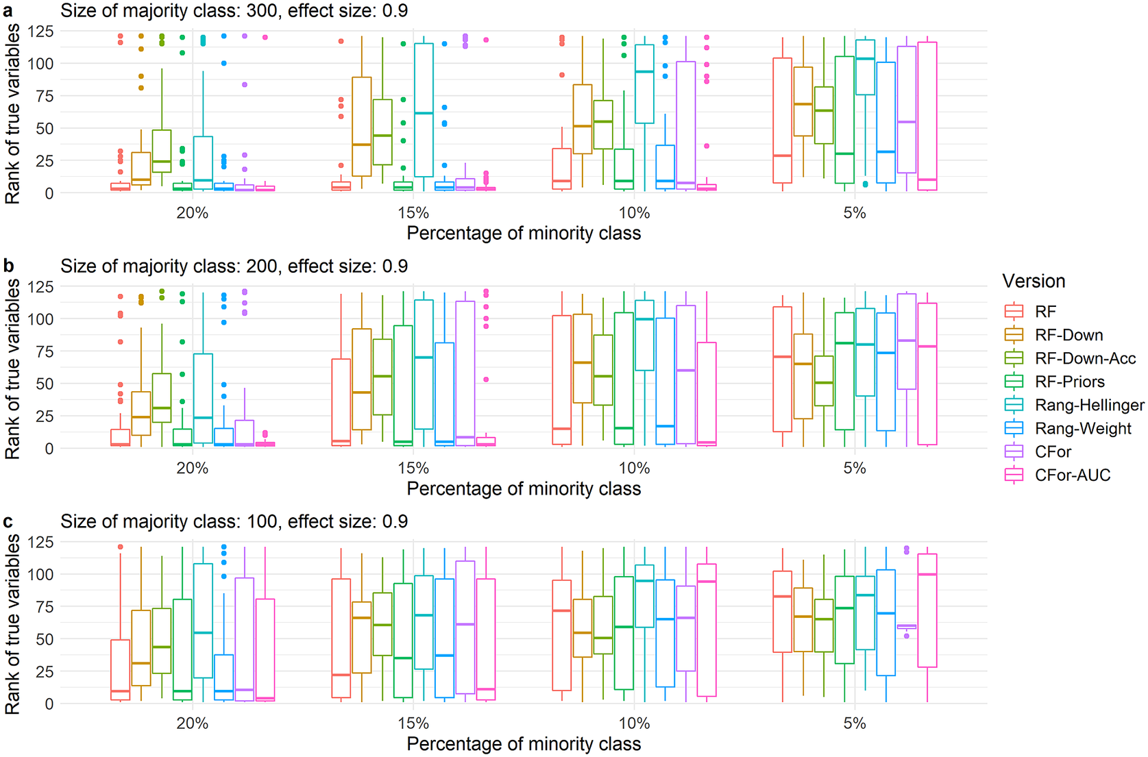
Figure 4. Boxplots showing ranks of permutation importance for four true variables with low VIFs and a medium effect size of 0.9. For each of the 60 simulated test sets with a total of 121 covariates, permutation importance was calculated 10 times for each of the eight algorithm versions. The true predictors were ranked by the mean permutation importance averaged over the 10 repetitions. Boxes showing interquartile range and median; whiskers show the maximum of 1.5 × interquartile range. Boxes represent the eight algorithm versions: default RF (RF), two downsampled versions (RF-Down, RF-Down-Acc), priors representing the proportion of class sizes (RF-Priors), Hellinger distance as splitting criterion (Rang-Hellinger), weighted random forest (Rang-Weight), random forest based on conditional inference trees (CFor), AUC permutation importance (CFor-AUC; from left to right). Sample sizes decrease from row a to row c. Imbalance levels increase from left to right.
Similarly, for high effect sizes of 1.4, the AUC permutation importation importance ranked true variables still highly for smaller sample sizes and higher imbalance levels when the other seven algorithm versions no longer did (Figure 5 and Supplementary Figure S3). The versions based on Hellinger distance and downsampling produced lower ranks for true variables sooner as sample sizes decreased and imbalance levels increased compared to the other five algorithm versions. For all algorithm versions, the performance decreased as the number of true variables increased or the VIFs of true variables increased. Compared to true variables with medium effects sizes, true variables with high effect sizes were often still ranked highly at sample sizes and imbalance levels at which true variables with medium effect sizes no longer were ranked highly (Supplementary Figures S2 and S3). For low effect sizes of 0.4, all algorithm versions produced low ranks for true variables in most situations and only for the highest sample sizes and lowest imbalance levels and with few true variables did the four algorithm versions AUC permutation importance, default RF and the versions based on priors and weights rank true variables relatively highly (Supplementary Figure S4). Reversing the class weights in Rang-Weight had little effect on the ranking of true variables, but ranks of true variables were substantially lower when reversing the class priors in RF-Priors (Supplementary Figure S5).

Figure 5. Boxplots showing ranks of permutation importance for true variables with a high effect size of 1.4. For each of the 360 simulated test sets with a total of 121 covariates, permutation importance was calculated 10 times for each of the eight algorithm versions. The true predictors were ranked by the mean permutation importance averaged over the 10 repetitions. The boxplots summarize the ranking across all true variables with high effect sizes of 1.4 across simulated data with one, two, and four true variables and with low and with high VIFs of the true variables. Boxes showing interquartile range and median; whiskers show the maximum of 1.5 × interquartile range. Boxes represent the eight algorithm versions: default RF (RF), two downsampled versions (RF-Down, RF-Down-Acc), priors representing the proportion of class sizes (RF-Priors), Hellinger distance as splitting criterion (Rang-Hellinger), weighted random forest (Rang-Weight), random forest based on conditional inference trees (CFor), AUC permutation importance (CFor-AUC; from left to right). Sample sizes decrease from row a to row c. Imbalance levels increase from left to right.
At the sample sizes, imbalance levels, number of true variables, VIFs of true variables, and effect sizes at which the AUC permutation importance produced higher ranks than the default RF permutation importance, sensitivity in variable selection increased when the AUC permutation importance was used to rank all covariates. Using AUC instead of OOB as the criterion in variable selection increased sensitivity in variable selection even further at higher sample sizes and imbalance levels. Specificity showed a slight reverse trend among the two versions based on AUC permutation importance, but was relatively high overall (Figure 6).
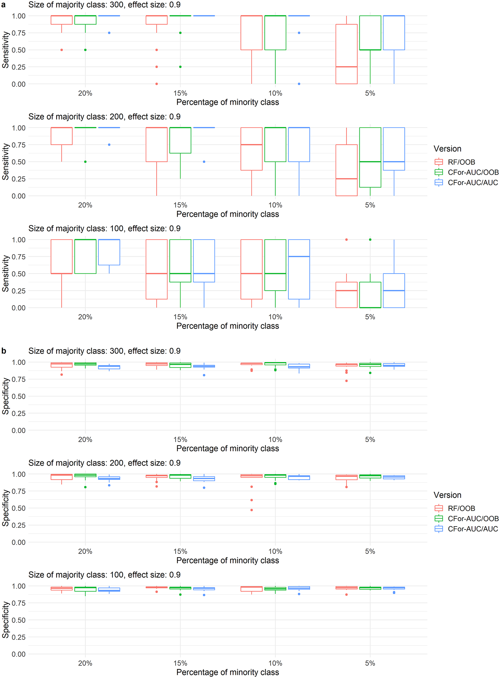
Figure 6. Boxplots of (a) sensitivity and (b) specificity of variable selection for three alternative variable selection approaches with random forest. Variable selections were implemented for simulated data with 121 covariates including one, two, or four covariates with a medium effect size of 0.9 and with low variable inflation factors. Sensitivity represents the rate at which true covariates are identified. Specificity represents the rate at which noise covariates are rejected. Boxes represent from left to right (1) RF/OOB: the default variable selection approach with no adjustments for unbalanced data, (2) CFor-AUC/OOB: covariates are ranked by the AUC permutation importance instead of the default permutation importance, and (3) CFor-AUC/AUC: covariates are ranked by the AUC permutation importance and the threshold criterion in the forward selection is AUC instead of OOB. Boxes showing interquartile range and median, whiskers show the maximum of 1.5 × interquartile range, dots: outliers.
3.2. Case studies
The final models for the distributions of the three breeding waders (Figure 7) contained covariates at scales between 0.25 and 10 km (Table 1). At finer spatial scales the models identified species–habitat relationships we expected to find based on previous knowledge about the species. At fine scales similar to the home ranges of the species (250 m), all species had an association to wetter conditions: for Northern lapwing to moist soils, for common snipe to soils with impeded drainage and for common redshank we found an association to a satellite data vegetation index (IVR) which has been linked to marshes (Table 1). Northern lapwings avoided elevations of 200–300 m, which in the study area are dominated by bottoms of major valleys and intensive spring grazing, hence our model indicated an avoidance of improved pastures. As expected for Northern lapwings, our model also showed that Northern lapwings avoided steep slopes and preferred gentle slopes (Table 1).

Figure 7. Predicted probability of (a) Northern lapwing, (b) common snipe, and (c) common redshank presence in the study area. Only areas below 500 m elevation shown, which were those surveyed. Also shown is whether these species were recorded on the transects. Maps derived: using NATMAP soilscapes Cranfield University (NSRI) and for the Controller of HMSO 2009, Land-Form PANORAMA, OS MasterMap, Strategi data downloaded from the EDINA Digimap OS service. Crown Copyright/ database right 1993, 2007, and 2009. An Ordnance Survey / EDINA supplied service, Landsat Surface Reflectance products courtesy of the U.S. Geological Survey Earth Resources Observation and Science Center.
Table 1. Selected multi-scale covariates in models for Northern lapwing, common snipe, and common redshank in the Yorkshire Dales, UK.

Note. Rank refers to the position of the covariate when ordered by mean permutation importance. Relationship: Directions of the species–habitat relationships were inferred from partial dependence plots of a random forest model. +, Probability of species presence increased with higher values of the covariate. −, Probability of species presence decreased with higher values of the covariate. (), considerable variation in the overall trend. U, Probability of a species presence increased with lower and higher values of the covariate and decreased with intermediate values.
The models suggested several species–habitat relationships for the less well-studied coarser scales. Aspect was frequently selected at scales of 5–10 km (Table 1). Partial dependence plots suggested that relationships of breeding common snipe with west-facing aspect at a scale of 7 km were negative. Relationships of all three species with either north, north-east, east, south-east, or south-facing aspects were positive at scales of 5–10 km. At scales of 5–10 km, all species had a positive relationship to the area of wet soils. Northern lapwing and common redshank had a positive relationship with gently sloping (2–5°) land at the 7–10 km scale.
4. Discussion
With unbalanced data and random forest, the majority class may be predicted with a higher accuracy than the minority class and permutation importances may be biased (Chen et al., Reference Chen, Liaw and Breiman2004; Lin and Chen, Reference Lin and Chen2012; Janitza et al., Reference Janitza, Strobl and Boulesteix2013). For variable rankings based on simulated data we found that the AUC permutation importance was least affected by data imbalance out of eight alternative algorithm versions. All eight algorithm versions ranked true variables lower and more variably as sample size decreased, the imbalance level increased, the number of true variables increased, their effect sizes decreased or their VIFs increased. For the same number of true variables, effect sizes, and VIFs, the AUC permutation importance ranked true variables still highly at sample sizes and imbalance levels at which the other seven algorithms did not. Conversely, the version with the Hellinger distance and the two downsampling versions already ranked true variables lower and more variably at sample sizes and imbalance levels at which the other five algorithms still ranked true variables highly. Higher ranking of true variables with the AUC permutation importance lead to a higher proportion of true variables identified during variable selection compared to the default permutation importance. Sensitivity increased further when the AUC instead of the OOB error was used as the criterion in the forward variable selection. The sample sizes and imbalance levels in our simulated data are typical for some national monitoring programmes of species (Schmid et al., Reference Schmid, Zbinden and Keller2004; Snäll et al., Reference Snäll, Kindvall, Nilsson and Pärt2011). Within the field of species distribution modeling, our results can therefore be relevant for data from national or regional studies (see our case studies) and outside of species distribution modeling for data with similar sample sizes and imbalance levels as in our simulated data.
Even the highest performing algorithm version, the AUC permutation importance failed to rank true variables highly at the lowest sample sizes and highest imbalance levels and consequently failed to achieve a high sensitivity in the identification of true variables during variable selection. When the absolute number of cases of the minority class is very low, the corresponding lack of information cannot be overcome with improvements to the calculation of variable importances (Janitza et al., Reference Janitza, Strobl and Boulesteix2013). Nonetheless, our results for the AUC permutation importance suggest that when VIFs of true variables were low and the classification problems relatively simple (1–2 true variables, medium effect sizes), as few as 10–20 cases for the minority class were sufficient to achieve high ranks of true variables despite data imbalance and despite a large number of covariates relative to sample size. With high effect sizes and 1–2 true variables, even as few as five cases for the minority class were at times sufficient to rank true variables highly. When VIFs of true variables are high, analysts may be able to increase their success of correctly ranking covariates by manually eliminating covariates with high VIFs before a ranking of covariates with random forest. However, in the subsequent interpretation of results, it may be important to consider that highly ranked covariates may then be only proxies for true drivers that were manually eliminated. When the aim of a study is to find many of the important variables associated with a response variable (Nicodemus et al., Reference Nicodemus, Malley, Strobl and Ziegler2010; Genuer et al., Reference Genuer, Poggi and Tuleau-Malot2015), a preselection of covariates with low VIFs may not be desirable.
Downsampling and use of the Hellinger distance in node splits resulted not only in lower average ranks of true variables at sample sizes and imbalance levels at which the five other algorithm versions still produced high ranks, but also in highly variable ranking of true predictors, which impedes unbiased variable selection and inference. In our simulations, we averaged permutation importances over 10 repetitions of a random forest model using a relatively high number of trees (2,000). In studies in which permutation importances from a single random forest model are used, the variability in importance measures will likely be higher. In contrast to our results based on variable ranking, (Valavi et al., Reference Valavi, Elith, Lahoz-Monfort and Guillera-Arroita2021a) found that downsampling and the Hellinger distance combined with shallow trees produced the highest discrimination between classes. Their sample sizes were higher compared to our study, which may limit the risk of information loss in downsampling. They suggested that further research is needed to investigate the contributions of the Hellinger distance as splitting criterion versus tree depth to the improvement in discriminative ability. We found that reversing the weights in Rang-Weight had little effect on the ranking of true variables, suggesting not only that no fine-tuning of weights is necessary for variable ranking, but also that the weighing may have little effect on variable ranking. Conversely, reversing the priors resulted in substantially lower rankings of true variables.
Nonlinear covariate effects and interactions among covariates are common in environmental sciences, including species distribution modeling (Franklin, Reference Franklin2009). Random forest learns nonlinearities and interactions from the data without the need to explicitly specify these (Grömping, Reference Grömping2009). Our simulations were based on covariate effects that were linear (at the scale of the linear predictor) and additive. Further research is necessary to investigate if the AUC permutation importance performs better compared to other approaches also in more complex situations that involve covariate interactions and nonlinear effects.
Our simulation and case studies considered random forest for classification. Data imbalance may also be an issue in random forest for regression. Few datapoints in a region of interest in environmental space may result in poor predictive performance for the region of interest (Branco et al., Reference Branco, Torgo and Ribeiro2017). Strategies to improve predictive performance in the area of interest with random forest for regression are less well-researched compared to the problem of unbalanced data in random forest for classification (Branco et al., Reference Branco, Torgo and Ribeiro2017).
4.1. Case studies
The results from our case studies suggest that our models correctly identified a number of known species–habitat relationships despite the problems of unbalanced data. Habitat selection at finer spatial scales such as home ranges is well-studied for all three species (e.g., Baines, Reference Baines1990; Green et al., Reference Green, Hirons and Cresswell1990; O’Brien, Reference O’Brien2002; Taylor and Grant, Reference Taylor and Grant2004; Smart et al., Reference Smart, Gill, Sutherland and Watkinson2006; Sharps et al., Reference Sharps, Garbutt, Hiddink, Smart and Skov2016). At this scale, our models identified species–habitat relationships consistent with previous studies. We found preferences for wet conditions in all species, which has previously been found (Green et al., Reference Green, Hirons and Cresswell1990; O’Brien, Reference O’Brien2002; Smart et al., Reference Smart, Gill, Sutherland and Watkinson2006). We also found that Northern lapwing preferred gentle over steep slopes and that they avoided improved pastures, consistent with previous studies (Henderson et al., Reference Henderson, Wilson, Steele and Vickery2002; Taylor and Grant, Reference Taylor and Grant2004).
At coarser spatial scales, less knowledge about species–habitat relationships is available. Based on the case studies, we suggest the following hypotheses about processes at larger spatial scales: First, all species showed a positive relationship to south-facing aspects and common snipe had a negative relationship to a west-facing aspect. The birds may be selecting for warmer microclimates with higher solar irradiation (south-facing aspects) and avoiding the strong westerly wind (Met Office, 2015). Whinchat (Saxicola rubetra) also favored south and east-facing aspects (for home ranges) (Calladine and Bray, Reference Calladine and Bray2012). This was hypothesized to be linked to higher food availability in warmer aspects. In the hilly landscape of the Yorkshire Dales, small patches can be sheltered from wind or sun by local topography, and the relationship may only be revealed at coarser spatial scales. Second, at the 10 km scale, we found that Northern lapwing was associated with gentle slopes (2°–5°). In the prebreeding period, female-dominated Northern lapwing flocks forage in fields with high earthworm densities (often improved fields) and later nest in surrounding fields (Baines, Reference Baines1990) preferring gentle slopes (Taylor and Grant, Reference Taylor and Grant2004) and avoiding improved pastures (Henderson et al., Reference Henderson, Wilson, Steele and Vickery2002). The positive relationship with gentle slopes at the 10 km scale may thus reflect a preference for the wider valleys of the Yorkshire Dales, which offer more areas with a gentle slope outside of intensively grazed valley bottoms in combination with many potential prebreeding foraging fields in the vicinity. Third, there was a positive relationship with wet soil at coarser spatial scales for all species. A positive relationship with wet conditions at the scale of home ranges is well known for all three species (Green et al., Reference Green, Hirons and Cresswell1990; O’Brien, Reference O’Brien2002; Smart et al., Reference Smart, Gill, Sutherland and Watkinson2006). In landscapes with more abundant wet areas, habitat unoccupied in other landscapes may be used, because pairs are less dependent on the quality of a single small area if the surroundings offer opportunities to supplement resources. Alternatively, in landscapes with abundant wet areas and consequently a higher density of breeding pairs, conspecific attraction may lead to increased settlement. There is evidence from some bird species, that areas with higher breeding densities attract more immigrants (Doligez et al., Reference Doligez, Pärt, Danchin, Clobert and Gustafsson2004). The modeled species–habitat relationships only reveal patterns, not causation and the new hypotheses will need to be tested in additional studies (Dormann et al., Reference Dormann, Schymanski, Cabral, Chuine, Graham, Hartig, Kearney, Morin, Römermann, Schröder and Singer2012).
The importance of considering multiple spatial scales of environmental covariates to derive accurate species distribution maps is well known and reflects that multiple-scale processes are shaping species distributions (Wiens, Reference Wiens1976; Johnson, Reference Johnson1980; Addicott et al., Reference Addicott, Aho, Antolin, Padilla, Richardson and Soluk1987; Wiens et al., Reference Wiens, Rotenberry and Van Horne1987; Wiens, Reference Wiens1989; Levin, Reference Levin1992; Thogmartin and Knutson, Reference Thogmartin and Knutson2007; Mateo-Tomas and Olea, Reference Mateo-Tomas and Olea2009; Jackson and Fahrig, Reference Jackson and Fahrig2012; Bellamy et al., Reference Bellamy, Scott and Altringham2013; Bradter et al., Reference Bradter, Kunin, Altringham, Thom and Benton2013; Bellamy and Altringham, Reference Bellamy and Altringham2015; Galitsky and Lawler, Reference Galitsky and Lawler2015; McGarigal et al., Reference McGarigal, Wan, Zeller, Timm and Cushman2016). Our multi-scale models revealed that, at least in the case of the three wader species, conservation policy and delivery may need to consider approaches that work at the scale of farm clusters or even whole valleys bringing together groups of landowners to support wader populations over wider areas.
Abbreviations
- AUC
-
area under the curve
- CFor
-
random forest based on conditional inference trees
- CFor-AUC
-
AUC permutation importance in random forest based on conditional inference trees
- CFor-AUC/AUC
-
variable selection in which variables are ranked based on the AUC permutation importance and AUC is used as the threshold criterion in forward variable selection
- CFor-AUC/OOB
-
variable selection in which variables are ranked based on the AUC permutation importance and OOB error is used as the threshold criterion in forward variable selection
- mtry
-
the number of variables tried at each node split
- ntree
-
the number of trees in a forest
- OOB
-
out-of-bag
- Rang-Hellinger
-
random forest with the Hellinger distance as splitting criterion
- Rang-Weight
-
random forest with weights to account for differences in class size
- RF
-
random forest with no adjustment for unbalanced data
- RF-Down
-
random forest in which the majority class is downsampled to the size of the minority class
- RF-Down-Acc
-
random forest in which the majority class is downsampled to 64% of the size of the minority class
- RF/OOB
-
variable selection with no adjustment for unbalanced data. Variables are ranked based on the permutation importance and OOB error is used as the threshold criterion in forward variable selection
- RF-Priors
-
random forest with priors to account for differences in class size
Author Contributions
U.B. conceived the idea, collected the survey data, carried out the analysis, and wrote the first draft. T.G.B., J.D.A., W.E.K., and T.J.T. advised on study design and analysis. J.O. advised on remotely sensed data and their acquisition. All authors contributed to the final version.
Competing Interests
The authors declare no competing interests exist.
Data Availability Statement
The simulated data and the bird survey data are available on Zenodo: http://doi.org/10.5281/zenodo.7337856. The GIS data described in Supplementary Appendix S1 are available from Digimap: https://digimap.edina.ac.uk, the Met office: www.metoffice.gov.uk, the U.S. Geological Survey Earth Resources Observation and Science Center: http://landsat.usgs.gov and the National Soil Resources Institute: www.landis.org.uk. R code is provided in the Github repository: https://github.com/UteBradter/Unbalanced_RandomForest.
Funding Statement
The study was funded by the Yorkshire Dales National Park Authority, the Biotechnology and Biological Sciences Research Council (Reference number: BB/J005851/1), and the Nigel Bertram Charitable Trust.
Supplementary Materials
To view supplementary material for this article, please visit http://doi.org/10.1017/eds.2022.34.


 Open access