
Introduction
Many years have passed since the publications of Systema Naturae (Linnaeus 1735) and On the Origin of Species (Darwin Reference Darwin1859), but consensus about the species concept remains elusive (de Queiroz Reference de Queiroz2007, Hausdorf Reference Hausdorf2011, Barrowclough et al. Reference Barrowclough, Cracraft, Klicka and Zink2016, Burfield et al. Reference Burfield, Butchart and Collar2017). Nevertheless, species level taxonomy dominates conservation and management policy and practice, e.g. the US Endangered Species Act (U.S. Fish & Wildlife Service 1973), the Birds Directive of the EU (EU 2009) and the IUCN Red List of Threatened Species (IUCN 2017). Even with a pragmatic approach, agreeing on “valid” species can be problematic, especially when novel technologies keep changing the resolution of the taxonomic landscape (Sites and Marshall Reference Sites and Marshall2004, Goldstein et al. Reference Goldstein, Wyner, Doukakis, Egan, Amato, Rosenbaum and DeSalle2005, Johnson et al. Reference Johnson, Watson and Mindell2005, Tobias et al. Reference Tobias, Seddon, Spottiswoode, Pilgrim, Fishpool and Collar2010, Baetu Reference Baetu2012). Also, strict species-level policies ignore within-species population structures, which are potentially significant for biodiversity conservation (Sullivan et al. Reference Sullivan, Douglas, Walker, Cordes, Davis, Anthonysamy, Sullivan and Douglas2014, Coetzer et al. Reference Coetzer, Downs, Perrin and Willows-Munro2015, Peters et al. Reference Peters, Lavretsky, DaCosta, Bielefeld, Feddersen and Sorensen2016). Increasingly though, below species-level population units are recognised in conservation and management, e.g. the “distinct population segments” of the Endangered Species Act and “flyway management units” of the African-Eurasian Waterbird Agreement (UNEP/AEWA) (Marjakangas et al. Reference Marjakangas, Alhainen, Fox, Heinicke, Madsen, Nilsson and Rozenfeld2015). We expect this trend to continue and spread, and, thus, the need for in-depth knowledge of population structures to increase.
After several decades of unprecedented increase in large avian herbivore numbers across the northern hemisphere (Ankney Reference Ankney1996, Fox et al. Reference Fox, Ebbinge, Mitchell, Heinicke, Aarvak, Colhoun, Clausen, Dereliev, Faragó, Koffijberg, Kruckenberg, Loonen, Madsen, Mooij, Musil, Nilsson, Pihl and van der Jeugd2010), their management has become an urgent topic (Hake et al. Reference Hake, Månsson and Wiberg2010, Madsen et al. Reference Madsen, Guillemain, Nagy, Defos du Rau, Mondain-Monval, Griffin, Williams, Bunnefeld, Czajkowski, Hearn, Grauer, Alhainen and Middleton2015). Large avian herbivores, e.g. geese, deliver a wide range of ecosystem services (Green and Elmberg Reference Green and Elmberg2014), but can also cause damage and nuisance (Owen Reference Owen1990, Jefferies and Rockwell Reference Jefferies and Rockwell2002). Outside the breeding season, they frequently mix in multi-species gatherings, making species-level monitoring and impact evaluations, and thus, evidence-based control and management programmes, difficult to implement (MacMillan et al. Reference MacMillan, Hanley and Daw2004). Species with unfavourable conservation status run an obvious risk of paying a devastating toll in harvesting and crop-protection schemes targeting these avian herbivore communities at large, e.g. when protected geese are shot unintentionally during hunts of geese with similar appearance or in scaring off mixed species flocks. A similar situation occurs when species contain multiple subpopulations with different sizes and trends, and thus, conservation status. If these subpopulations are not treated separately, units with poor conservation status risk to be harmed by species-level policies, e.g. under the Birds Directive of the EU (EU 2009) or national hunting regulations. Loss of below species-level biodiversity could very well reduce ecosystem services and resilience (Ryder Reference Ryder1986, Zink Reference Zink2003, Díaz et al. Reference Díaz, Fargione, Stuart Chapin and Tilman2006).
Outside the breeding season, the Bean Goose Anser fabalis is found in multi-species assemblies on agricultural land in temperate Eurasia (del Hoyo et al. Reference del Hoyo, Elliott and Sargatal1992). Unlike most of its guild members, Bean Goose numbers have decreased in recent times (Fox et al. Reference Fox, Ebbinge, Mitchell, Heinicke, Aarvak, Colhoun, Clausen, Dereliev, Faragó, Koffijberg, Kruckenberg, Loonen, Madsen, Mooij, Musil, Nilsson, Pihl and van der Jeugd2010, IUCN 2017). In many European countries it is still a hunted species, and it is also subject of crop-protection measures through scaring and shooting (Fox and Madsen Reference Fox and Madsen1997, Hake et al. Reference Hake, Månsson and Wiberg2010, Månsson et al. Reference Månsson, Risberg, Ängsteg and Hagbarth2015, Fox et al. Reference Fox, Elmberg, Tombre and Hessel2016a). Throughout its huge range, the Bean Goose exhibits a high level of variation in breeding habitat, migration routes, morphology and genetics. For these reasons, the Bean Goose is a challenging species for evidence-based conservation and management at the combined multi-species, species and subspecies levels (“pan-taxonomic level”).
The taxonomy of the Bean Goose and its relationship to nearby species has long been debated (Delacour Reference Delacour1951, Sangster and Oreel Reference Sangster and Oreel1996, Sangster et al. Reference Sangster, Hazevoet, van den Berg, Roselaar and Sluys1999, Ruokonen and Aarvak Reference Ruokonen and Aarvak2011, Honka et al. Reference Honka, Kvist, Heikkinen, Helle, Searle and Aspi2017). The Pink-footed Goose Anser brachyrhynchus is now considered to be genetically distinct from A. fabalis (Ruokonen et al. Reference Ruokonen, Litvin and Aarvak2008, but see Delacour Reference Delacour1951), although recently, Ottenburghs et al. (Reference Ottenburghs, Megens, Kraus, Madsen, van Hooft, van Wieren, Crooijmans, Ydenberg, Groenen and Prins2016) placed A. brachyrhynchus as a sister species of the (split off) Tundra Bean Goose A. serrirostris. Other Anser geese are also considered closely related to the Bean Goose (Ruokonen et al. Reference Ruokonen, Kvist and Lumme2000). Clearly, taxonomic revision is ongoing in this genus.
Below species level, the number of proposed subspecies has varied over time (Ruokonen and Aarvak Reference Ruokonen and Aarvak2011 for a review), but currently a system of four subspecies is most commonly accepted: two tundra forms (Eastern A. f. serrirostris and Western A. f. rossicus) and two taiga forms (Eastern A. f. middendorffii and Western A. f. fabalis). Meanwhile, species status has been suggested for most of these subspecies, either alone or in combination with others (Burgers et al. Reference Burgers, Smit and van der Voet1991, Sangster and Oreel Reference Sangster and Oreel1996, Ruokonen et al. Reference Ruokonen, Litvin and Aarvak2008, Ottenburghs et al. Reference Ottenburghs, Megens, Kraus, Madsen, van Hooft, van Wieren, Crooijmans, Ydenberg, Groenen and Prins2016). Given the status of ‘species’ in national and international legislation and agreements, this situation is unsatisfactory. UNEP/AEWA avoided much of this controversy by agreeing on an International Single Species Action Plan (ISSAP) for the (Western) Taiga Bean Goose, yet accepting the subspecies status of this taxon (Marjakangas et al. Reference Marjakangas, Alhainen, Fox, Heinicke, Madsen, Nilsson and Rozenfeld2015, see also Madsen and Williams Reference Madsen and Williams2012).
This Taiga Bean Goose ISSAP preliminarily recognizes three flyway units in Europe (Western, Central and Eastern I), thus further differentiating the population structure (Marjakangas et al. Reference Marjakangas, Alhainen, Fox, Heinicke, Madsen, Nilsson and Rozenfeld2015). The ISSAP also points at an urgent need for evidence to support the delineation of these flyway units. Fox et al. (Reference Fox, Hobson, de Jong, Kardynal, Koehler and Heinicke2016b) used multi-element feather stable isotope analyses to support the delineation of these flyway units, but genetic support is still missing. Also, there is no evidence to support that the proposed level of population structure, expressed by separate flyways, is the optimal level for conservation and management. On the contrary, neckband sightings and location data from GPS/GSM-tagged individuals suggest that further refinement is needed (de Jong and Nilsson Reference de Jong and Nilsson2016, Kroglund and Østnes Reference Kroglund and Østnes2016, Mitchell et al. Reference Mitchell, Griffin, Maciver, Minshull and Makan2016).
Taiga Bean Geese perform annual migrations over thousands of kilometres and, across its range, in diverse directions (Nilsson et al. Reference Nilsson, de Jong and Heinicke2009, Marjakangas et al. Reference Marjakangas, Alhainen, Fox, Heinicke, Madsen, Nilsson and Rozenfeld2015). During these movements, individuals from across the breeding range regularly use the same areas for staging or wintering (Nilsson Reference Nilsson2013, Arzel et al. Reference Arzel, Elmberg and Guillemain2006). Strong pair bonds are commonplace in geese, but unfortunately the timing of pair formation, and thus its role in gene flow and population structuring in Taiga Bean Goose, is unknown. Well-known are the strong family bonds (the young stay with their parents for almost a full annual cycle) and the social structure of goose flocks (Prevett and MacInnes Reference Prevett and MacInnes1980, Ely Reference Ely1993). In these social networks, experience is gathered and shared to form traditions, e.g. in movement patterns and phenology (Raveling Reference Raveling1979). When different assemblies develop different patterns, this could lead to population structuring. Taiga Bean Geese are flightless for a few weeks during the moulting period in June-August. Adults with chicks moult in their breeding territories, but the rest gather at specific moulting sites (Salomonsen Reference Salomonsen1968, Nilsson et al. Reference Nilsson, de Jong and Sjöberg2008, Reference Nilsson, de Jong, Heinicke and Sjöberg2010, de Jong Reference de Jong2013). If geese from various breeding regions meet at those moulting sites, genetic admixture could occur. In summary, over the course of their life cycle, there are life history traits that could promote small-scale genetic structure and other traits that could counteract this.
In this study, we examine genetic diversity and structure in Central Scandinavian Taiga Bean Goose, representing a subset of the Western Flyway Unit (Marjakangas et al. Reference Marjakangas, Alhainen, Fox, Heinicke, Madsen, Nilsson and Rozenfeld2015). The aim is to add knowledge about fine-scale genetic variation in the light of pan-taxonomic conservation and management of geese. The role of fine-scale genetic variation is probably important for many bird species, particularly those in need of conservation measures.
Materials and methods
Study population
The Taiga Bean Goose breeds across a discontinuous range in the northern boreal zone, from Scandinavia into the West-Siberian Lowlands (Fox et al. Reference Fox, Ebbinge, Mitchell, Heinicke, Aarvak, Colhoun, Clausen, Dereliev, Faragó, Koffijberg, Kruckenberg, Loonen, Madsen, Mooij, Musil, Nilsson, Pihl and van der Jeugd2010). Within this range, four flyway units have been preliminarily accepted, of which three occur in Europe (Marjakangas et al. Reference Marjakangas, Alhainen, Fox, Heinicke, Madsen, Nilsson and Rozenfeld2015). With an estimated population size of 1,500 individuals, the Western Flyway Unit (WFU) is the least numerous of these units. Its breeding range spans from Dalarna County northward through western Sweden and adjacent parts of Norway, but in most of this range, the occupancy appears to be patchy (Svensson et al. Reference Svensson, Svensson and Tjernberg1999, Marjakangas et al. Reference Marjakangas, Alhainen, Fox, Heinicke, Madsen, Nilsson and Rozenfeld2015). Breeding Taiga Bean Geese have been studied in Nord-Trøndelag County in Norway (Kroglund and Østnes Reference Kroglund and Østnes2016) and Södra Lappland region in Sweden (Parslow-Otsu Reference Parslow-Otsu1991, Parslow-Otsu and Kjeldsen Reference Parslow-Otsu and Kjeldsen1992, Svensson et al. Reference Svensson, Svensson and Tjernberg1999, Nilsson et al. Reference Nilsson, de Jong and Sjöberg2008). Although these areas are geographically close by, the Scandic Mountain Range splits the distribution into two ecologically separated clusters. Recent work in these areas, e.g. with GPS/GSM neck-collars, has shown that individuals from these clusters share wintering and moulting areas, but that their migration routes and staging sites differ (de Jong and Nilsson Reference de Jong and Nilsson2016, Kroglund and Østnes Reference Kroglund and Østnes2016).
Sample collection and DNA extraction
Blood, feather and faecal samples were collected during spring and summer at three locations from 2010 to 2016 (Table 1). Geese were caught with cannon nets at spring staging sites in Røyrvik municipality in 2010 and 2013 and by herding flightless moulting flocks (> 70 to > 300 individuals) into standing nets at the Stalon and Nästansjö sites in 2012 and 2015. These catching sites were chosen on the basis of known occurrences (Nilsson et al. Reference Nilsson, de Jong and Sjöberg2008, Kroglund and Østnes Reference Kroglund and Østnes2016), but without prior knowledge of potential population structure. In addition to sampling live birds, shed feathers and droppings were collected opportunistically during scouting trips within breeding and moulting areas. In six cases, subsequent analyses showed that individual geese had been sampled in the Røyrvik breeding area and the Stalon moulting site. These individuals were geographically assigned to their breeding area. The location of the settlements Røyrvik, Stalon and Nästansjö are 64.89oN/13.56oE, 64.93oN/15.88oE and 64.79oN/16.52oE respectively, but we keep the exact locations of the nearby breeding and moulting sites secret in order to reduce the risk of human disturbance.
Table 1. Distribution of the N = 109 unique DNA samples over sites, years and sample types.
Genomic DNA was extracted from feathers using the Maxwell® 16 Research System (Promega, Madison, WI, USA) and the Maxwell 16 tissue DNA Purification Kit. Genomic DNA from blood samples was extracted with either the method above or using Qiagen’s Blood and Tissue Kit (Qiagen, Hilden, Germany). Genomic DNA from faecal samples was extracted using FastDNA Spin Kit for Soil (MP Biomedicals, Santa Ana, CA, USA).
Microsatellite genotyping
All samples were genotyped at 13 autosomal microsatellite loci and one sex-typing marker. The autosomal loci used included one locus previously developed from the Greater White-fronted Goose Anser albifrons (Aalµ1; Fields and Scribner Reference Fields and Scribner1997) and 12 loci previously developed from the Bean Goose (Kleven et al. Reference Kleven, Kroglund and Østnes2016). The Z-002A marker (Dawson Reference Dawson2007) was added to sex the samples. Loci were PCR-amplified with fluorescent-labelled forward primers (Applied Biosystems, Foster City, CA, USA) in two multiplexes as described in Kleven et al. (Reference Kleven, Kroglund and Østnes2016), and Aalµ1 (VIC labelled) was added to multiplex set b (see Table 2 in Kleven et al. Reference Kleven, Kroglund and Østnes2016). Multiplexing was performed with a Multiplex PCR Kit (Qiagen) following the manufacturer’s protocol, but using 8.4 µL reaction volume. PCR products (0.8 µL) were mixed with GeneScan 500 LIZ (Applied Biosystems) size standard (0.14 µL) and Hi-Di formamide (6.16 µL). PCR products were separated on an ABI 3130xl Genetic Analyzer and allele sizes assigned using GeneMapper software (Applied Biosystems).
Moulted feathers and faecal samples, like other types of non-invasively collected material, commonly have relatively low amounts and/or quality of DNA, which may result in genotyping errors such as the failure to amplify an allele (allelic dropout) or PCR-generated amplification of false alleles (Taberlet and Luikart Reference Taberlet and Luikart1999, Pompanon et al. Reference Pompanon, Bonin, Bellemain and Taberlet2005). To reduce the probability of genotyping errors, DNA from each moulted feather and faecal sample was analysed in three (or more if required) independent PCR replicates. We used ConGenR (Lonsinger and Waits Reference Lonsinger and Waits2015) to check for false alleles (FA rate = 0 in all loci) and allelic dropout rates. Based on the independent replicates, a locus-level consensus genotype was constructed using the following criteria: heterozygosity was accepted when at least two of the independent PCR-replicates showed heterozygosity, whereas homozygosity was only accepted when this was expressed in three independent PCRs. Samples that did not meet these requirements were omitted from the dataset. Samples with a consensus genotype containing at least 10 loci were used for individual identification with R-package Allelematch 2.5 (Galpern et al. Reference Galpern, Manseau, Hettinga, Smith and Wilson2012). The final dataset came to include 109 unique Taiga Bean Geese individuals, 19 of them represented by multiple consensus samples (17 from Røyrvik). Finally, we controlled the dataset for these 109 individuals for evidence of null alleles with Microchecker (Van Oosterhout et al. Reference Van Oosterhout, Hutchinson, Wills and Shipley2004).
Statistical analyses
First, we checked for global heterozygosity deficiency with Hardy-Weinberg U-test in Genepop 4.5.2 (Rousset Reference Rousset2008) and compared expected and observed heterozygosity with Arlequin 3.5.2.2 (Excoffier and Lischer Reference Excoffier and Lischer2010). Fstat 2.9.3.2 (Goudet Reference Goudet2001) was used to estimate allelic richness within sampling sites. Secondly, we analysed genetic distances between sampling sites by pairwise FST tests and AMOVA (in both cases using 99,999 permutations in Arlequin 3.5.2.2).
Thirdly, we explored the genetic structure among the samples. We used Structure 2.3.4 (Pritchard et al. Reference Pritchard, Stephens and Donnelly2000) with an admixture model (initial Alpha = 1.0) and independent allele frequencies and applied 100,000 burn-in steps, 1,000,000 repeats and 20 iterations. Test runs had shown that LnLikelihood stabilised within < 100,000 iterations and log(Alpha) showed weak levels of white noise across the range of repeats. We then used Structure Harvester Web 0.6.94 (Earl and vonHoldt Reference Earl and vonHoldt2012) to evaluate the number of clusters, and Clumpak (Kopelman et al. Reference Kopelman, Mayzel, Jakobsson, Rosenberg and Mayrose2015) to barplot averaged probabilities of cluster assignments. Supplementary to Structure, we used R package adegenet 2.0.1 (Jombart Reference Jombart2008, Jombart and Ahmed Reference Jombart and Ahmed2011) for cluster analyses and assignments. In addition to Bayesian clustering methods, we used GenAlEx 6.5 (Peakall and Smouse Reference Peakall and Smouse2012) for Principal Coordinate Analysis (PCoA). Finally, we calculated relatedness within and between sampling populations with ML-Relate (Kalinowski et al. Reference Kalinowski, Wagner and Taper2006).
Results
There was no evidence of false alleles for any of the 13 loci, and allelic dropout was observed in only three loci and at low rates (Afa02 = 0.0075, Afa25 = 0.0310 and Afa34 = 0.0074). Locus Afa18 showed evidence for a null allele and even failed to pass the global Hardy Weinberg equilibrium test. Consequently this marker was excluded from further analyses.
The Global Hardy-Weinberg U-test across all 12 loci and all samples (n = 109) showed no significant deficit of heterozygosity (P > 0.05). Across loci averaged observed heterozygosity (Ho) did not differ significantly from expected heterozygosity (He) for neither of the sampling sites (Table 2). Allelic richness was slightly lower among the Røyrvik samples compared with the Stalon and Nästansjö samples (Table 2).
Table 2. Measurements of genetic variation at 12 loci for samples from the three sampling sites: number of samples per site (n), observed average heterozygosity (HO), expected average heterozygosity (HE) and allelic richness ± SD (AR).
Pairwise FST between sampling sites showed a higher level of differentiation between the Røyrvik and Nästansjö samples (FST = 0.034, P < 0.001) than between the Røyrvik and Stalon samples (FST = 0.014, P < 0.01) and between the Nästansjö and Stalon samples (FST = 0.004, P > 0.05). Global AMOVA showed that 2% of the variation resulted from differences between populations and 98% from within populations (FST = 0.015, P < 0.001).
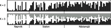
The results of the Structure analysis unveiled two or three genetic clusters among the 109 samples (Figure 1), with ΔK values favouring a split into two clusters (see Evanno et al. Reference Evanno, Regnaut and Goudet2005) (Figure 2). Adgenet results showed the lowest BIC values for three genetic clusters (Figure 3) and the sampled individuals were well separated in a scatterplot for these three clusters (Figure 4). Assigned against these three clusters, the individuals were non-randomly distributed over the sampling sites (χ23,3 P < 0.001). Cluster 1 dominated among the Røyrvik samples and cluster 3 among the Nästansjö samples, while cluster 2 was more evenly spread among the sampling sites (Table 3). A complex distribution of subpopulations across the sampling sites was also expressed in the results of the PCoA. Although the first three axes explained 19.6% of the overall variation, the sampling sites were not clearly separated when plotted against any pair of these three axes (Figure 5).
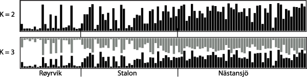
Figure 1. Assignment probability for individual Taiga Bean Geese on one of two (K = 2) or three (K = 3) clusters from Structure models.
Figure 2. Means of estimated Ln probabilities (A) and ΔK (B) across the number of Structure clusters (K).

Figure 3. Values of Bayesian Information Criterion (BIC) for 1 – 10 adegenet clusters on 40 retained Principal Components.
Figure 4. Scatterplot of individuals in the three clusters from the discriminant analysis of principal components (DAPC) analysis in adgenet. Retained Principal Components and Eigenvalues depicted in the insets.
Table 3. Number of individuals assigned to adegenet clusters 1, 2 and 3 across sampling sites.

Figure 5. PCoA plot of the individuals from the three sampling sites.
Within sampling sites, family relationships were more frequent among the Røyrvik samples than among the Stalon and Nästansjö samples (Table 4). Between sampling sites, family relationships were more common between Røyrvik and Stalon than between Røyrvik and Nästansjö (Table 4). The levels of relatedness within and between the Stalon and Nästansjö samples were similar (Table 4).
Table 4. Average relatedness (a) and relationship assignments (b) based on 12 microsatellite data within (bold) and between sampling areas: Røyrvik = R, Stalon = S and Nästansjö = N. Total number of pairs = 5,886.
Discussion
Genotyping errors were unlikely to have significantly influenced the results and the elimination of the poorly behaving Afa18 locus ensured that the HWE requirements were not violated. The Ho to He ratios and allelic richness for the three sampling sites were indicative of modest levels of genetic variation within the overall pool of samples.
Although the L(K) output of Structure showed very similar levels for K = 2 and K = 3 (Figure 2A), Structure Harvester suggested only two clusters in accordance with Evanno et al. (Reference Evanno, Regnaut and Goudet2005) (Figure 2B). Structure and Structure Harvester have been criticised for overemphasising K = 2, though (Janes et al. Reference Janes, Miller, Dupuis, Malenfant, Gorrell, Cullingham and Andrew2016). Based on Bayesian Information Criterion (BIC) levels, R program adegenet suggested three clusters (Figures 3 and 4). Until further data are available, we can only conclude that at least two subpopulations occur within this very restricted part of the Taiga Bean Goose range.
Individuals assigned to these clusters were unevenly distributed over the three sampling sites (Figure 1, Table 3), but the PCoA results showed that the samples from these three sites are not clearly separated (Figure 5). Viewed from a sampling site point of view, the genetic distance between the samples from Røyrvik and Nästansjö was larger than between those from Røyrvik and Stalon. The genetic distance between Stalon and Nästansjö was small. The AMOVA results showed that the samples from the three sites were significantly different, but that site contributed with only 2% of the overall genetic variation.
Our interpretation of these findings is that two or more subpopulations come together in the Stalon-Nästansjö moulting region. One of these subpopulations originates mainly from the Røyrvik breeding area and prefers the Stalon site. The link between Røyrvik and Stalon is confirmed by six cases of duplicate sampling and by the positions of four individuals tagged with GPS devices. These tagged individuals moved between the Røyrvik breeding area and the Stalon moulting site during multiple years (Kroglund and Østnes Reference Kroglund and Østnes2016, A. de Jong unpubl. data). Other individuals (n = 16) tagged with GPS devices at the Stalon and Nästansjö moulting sites proved to be Swedish residents and never visited Norway (A. de Jong unpubl. data).
Despite the incomplete sorting of subpopulations (clusters) between sampling areas, the genetic distance between the samples from Røyrvik and Nästansjö was in the same order of magnitude as those found between e.g. salmon populations of different rivers, differentiation levels commonly warranting genetic management units (Banks et al. Reference Banks, Rashbrook, Calavetta, Dean and Hedgecock2000, Ayllon et al. Reference Ayllon, Martinez and Garcia-Vazquez2006, Olafsson et al. Reference Olafsson, Pampoulie, Hjorleifsdottir, Gudjonsson and Hreggvidsson2014). Similar levels of FST values are also reported by Ely et al. (Reference Ely, Wilson and Talbot2017) for Greater White-fronted Goose populations along the Pacific Flyway and by Kvist et al. (Reference Kvist, Ponnikas, Belda, Encabo, Martínez, Onrubia, Hernández, Vera, Neto and Monrós2011) for three European subspecies of Reed Bunting Emberiza schoeniclus. We predict that, once the subpopulations found in our study can be properly assigned to breeding ranges, the genetic distances between these breeding populations will become important to consider in conservation and management policies.
Relatedness among individuals from the Røyrvik breeding area was high. Feathers and droppings (83% of the included Røyrvik samples) from family groups may have been sampled simultaneously, but even geographically and temporally separated samples were related. Our interpretation is that the observed level of relatedness mainly derived from the small population size of the Røyrvik group. This interpretation is supported by observational evidence, with a maximum of only 33 individuals observed within the pre-breeding staging area during recent years (Kroglund and Østnes Reference Kroglund and Østnes2016, J. E. Østnes unpubl. data).
High levels of relatedness can influence statistical analyses of genetic data (Palsbøl et al. Reference Palsbøl, Peery and Bérubé2010, Iacchei et al. Reference Iacchei, Ben-Horin, Selkoe, Bird, García-Rodríguez and Toonen2013, Putman and Carbone Reference Putman and Carbone2014). Preferably, the dataset should have been weeded for redundant family members, but our limited sample size did not allow this. Consequently, the results of our statistical analyses should be interpreted with this level of relatedness in mind. Meanwhile, for fine-scale genetic structure in a species with strong family bonds, relatedness is an unavoidable aspect. Relatedness and pedigree can also be used in further studies of the genetic structure and population size in Bean Goose and other bird species that are difficult to study during the breeding season (Økland et al. Reference Økland, Ariensen Haaland and Skaug2009, Creel and Rosenblatt Reference Creel and Rosenblatt2013). Our study has shown that non-invasive sampling (collection of faeces and feathers) can be used in this context.
Goose conservation and management deals with multi-species, multi-population systems, in which (genetic) management units can be game, pest or red-listed; sometimes all at once. They may also be trans-border migrants, and their ecology and demography poorly understood. The task is truly challenging, but possible to fulfil (Tuvendal and Elmberg Reference Tuvendal and Elmberg2015). Currently, ‘species’ are the main unit of policy making and implementation, and goose count results are the main input into the decision-making process. Instead, we suggest that conservationists and managers combine information from counts, migration studies and analyses of stable isotope and genetic samples in the design and implementation of their pan-taxonomic effort. Low- or non-invasive methods for intensive, range-wide sampling and genotyping (e.g. sampling of shed feathers and eDNA) are available to facilitate the data input for fine-tuned biodiversity conservation and management.
For conservation ecology at large, the recognition of fine-scale genetic structures within species raises the question whether or not the appointed sub-populations are “evolutionarily significant units” (sensu Ryder Reference Ryder1986). Considering the difficulties in predicting the long-term significance of any genetic “unit”, we suggest that even fine-scale genetic variation, especially when supported by differences in ecological and behavioural traits, is viewed as an important aspect of biodiversity, meriting conservation effort and careful management.
Acknowledgements
We thank the landowners (Statens Fastighetsverk and the Hugoson family), the local NGO Vilhelmina Model Forest, and all the members of the catching teams (in particular Thomas Heinicke and Risto Karvonen) for making the Vilhelmina moult catches possible. The editors of Bird Conservation International and two anonymous reviewers helped to improve the manuscript. In Sweden, Bean Geese were caught under permissions NV-11604-11 and NV-03680-15 issued by the Swedish Environmental Protection Agency, and blood and feather samples were collected under permission A38-12 issued by Umeå Djurförsöksetiska Nämnd. In Norway, permissions for catching and sampling were approved by the Norwegian Animal Research Authority (NARA, ID 1775 and ref. 2011/64833) and the Norwegian Environment Agency (ref. 2012/1756). This research was financially supported by the Swedish Wetland Fund and the Swedish Association for Hunting and Wildlife Management (grants to AdJ), and the County administration in Nord-Trøndelag and the Norwegian Environment Agency (grants to JEØ & RTK).