


1. Introduction
Double concentric jets is a configuration enhancing the turbulent mixing of two jets, which is used in several industrial applications where the breakup of the jet into droplets due to flow instabilities is presented as the key technology. Combustion (i.e. combustion chamber of rocket engines, gas turbine combustion, internal combustion engines, etc.) and noise reduction (e.g. in turbofan engines) are the two main applications of this geometry, although the annular jets can also be found in some other relevant applications such as ink-jet printers or spray coating (Mata et al. Reference Mata, Abadía-Heredia, López-Martín, Pérez and Le Clainche2023).
The qualitative picture emerging from this type of flow divides the inner field of concentric jets in three different regions: (i) initial merging zone, (ii) transitional zone and (iii) merged zone, as presented in figure 1, that follows the initial sketch presented by Ko & Kwan (Reference Ko and Kwan1976). In the initial merging zone (i), just at the exit of the two jets, two axisymmetric shear layers (inner and outer boundary layer) develop and start to merge. In this region, we distinguish the inner and outer shear layers, related to the inner and outer jet streams. Then, most of the mixing occurs in the transitional zone (ii), that extends until the external shear layer reaches the centreline. Finally, in the merged zone (iii), the two jets are totally merged, modelling a single jet flow.

Figure 1. Sketch representing the three flow regimes in the near field of double concentric jets. Figure based on the sketches presented in Ko & Kwan (Reference Ko and Kwan1976) and Talamelli & Gavarini (Reference Talamelli and Gavarini2006).
Several parameters define the characteristic of this flow: the inner and outer jet velocities, the jet diameters, the shape and thickness of the wall separating both jets, the Reynolds number, the boundary layer state and thickness at the jet exit and the free-stream turbulence. Based on these parameters, it is possible to identify several types of flow behaviour, which can be related to the presence of flow instabilities.
Numerous studies have investigated the interaction between the inner and outer shear layers of the jet and their effect on the flow instability. Starting with Ko & Kwan (Reference Ko and Kwan1976), they postulated that the double concentric jet configuration could be considered as a combination of single jets. Nevertheless, Dahm, Frieler & Tryggvason (Reference Dahm, Frieler and Tryggvason1992) revealed, by means of flow visualisations, diverse topology patterns as function of the outer/inner jet velocity ratio, reflecting that the dynamics of the inner and outer jet shear layers was different from that in a single jet. Moreover, this study exhibited a complex interaction between vortices identified in both shear layers, affecting the instability mechanism of the flow. Subsequently, different flow regimes are recognised as a function of the outer/inner velocity ratio. For cases in which the outer velocity is much larger than the inner velocity, the outer shear layer dominates the flow dynamics (Buresti, Talamelli & Petagna Reference Buresti, Talamelli and Petagna1994), and a low frequency recirculation bubble can be spotted at the jet outlet (Rehab, Villermaux & Hopfinger Reference Rehab, Villermaux and Hopfinger1997). For still high outer/inner velocity ratios, the outer jet drives the flow dynamics, exciting the inner jet which ends up oscillating at the same frequency as the external jet. This trend is known as the lock-in phenomenon, identified by several authors (Dahm et al. Reference Dahm, Frieler and Tryggvason1992; Rehab et al. Reference Rehab, Villermaux and Hopfinger1997; da Silva, Balarac & Métais Reference da Silva, Balarac and Métais2003; Segalini & Talamelli Reference Segalini and Talamelli2011). Moreover, the oscillation frequency detected was similar to the one defined by a Kelvin–Helmholtz flow instability, generally encountered in single jets. When the outer/inner velocity ratio is similar, a von Kármán vortex street is detected near the separating wall, depicted in various investigations (Olsen & Karchmer Reference Olsen and Karchmer1976; Dahm et al. Reference Dahm, Frieler and Tryggvason1992; Buresti et al. Reference Buresti, Talamelli and Petagna1994; Segalini & Talamelli Reference Segalini and Talamelli2011). A wake instability affected the inner and outer shear layers, reversing the lock-in phenomenon. Finally, for small outer/inner velocity ratios, the inner jet presents its own flow instability in the shear layer, while a different flow instability was identified in the outer jet, as shown by Segalini & Talamelli (Reference Segalini and Talamelli2011).
The velocity ratio between jets has also an influence on noise attenuation, which was analysed experimentally by Williams, Ali & Anderson (Reference Williams, Ali and Anderson1969). It was observed that, for some given configurations, more noise attenuation was present than for the others, with a maximum between  $12$ and 15 dB.
Regarding the geometric configuration of the concentric jets, Buresti et al. (Reference Buresti, Talamelli and Petagna1994) detected the presence of an alternate vortex shedding when the separation wall thickness between the two jets was sufficiently large, also recognised by Dahm et al. (Reference Dahm, Frieler and Tryggvason1992) and Olsen & Karchmer (Reference Olsen and Karchmer1976). This finding was as well presented by Wallace & Redekopp (Reference Wallace and Redekopp1992), including the influence of the wall thickness and sharpness on the characteristics of the jet.
This vortex shedding has been theoretically analysed (Talamelli & Gavarini Reference Talamelli and Gavarini2006) by means of linear stability analysis, and experimentally tested (Örlü et al. Reference Örlü, Segalini, Alfredsson and Talamelli2008). These investigations agree on the vortex shedding driving the evolution of both outer and inner shear layers. Consequently, a global absolute instability can be triggered by this mechanism with no external energy input. The vortex shedding can be therefore considered as a potential tool for passive flow control, delaying the transition to turbulence by means of controlling the near field of the jet.
The study performed in Talamelli & Gavarini (Reference Talamelli and Gavarini2006) constituted an entry point for subsequent research (although ignoring the effect of the duct wall separating the two streams). A similar procedure was employed to investigate the local linear spatial stability of compressible, inviscid coaxial jets (Perrault-Joncas & Maslowe Reference Perrault-Joncas and Maslowe2008), and lately accounting for the effects of heat conduction and viscosity (Gloor, Obrist & Kleiser Reference Gloor, Obrist and Kleiser2013). Both investigations found two modes of instability, one being associated with the primary and the other with the secondary stream, showing an independence between modes, the effect of velocity ratio mainly affects the first mode, while the second mode was primarily influenced by the diameter ratio between jets. Gloor et al. (Reference Gloor, Obrist and Kleiser2013) also identified parameter regimes in which the stability of the two layers is not independent anymore, and pointed that viscous effects are essential only below a specific Reynolds number. Subsequently, this work was expanded in Balestra, Gloor & Kleiser (Reference Balestra, Gloor and Kleiser2015) to investigate the local inviscid spatio-temporal instability characteristics of heated coaxial jet flows, where the presence of an absolutely unstable outer mode was identified.
Recently, Canton, Auteri & Carini (Reference Canton, Auteri and Carini2017) performed a global linear stability analysis to study more in detail this vortex-shedding mechanism behind the wall. They examined a concentric jet configuration with a very small wall thickness ( $0.1D$, with $D$ the inner jet diameter), but the authors selected an outer/inner velocity ratios where it was known that the alternate vortex shedding behind the wall was driving the flow. A global unstable mode (absolute instability) with azimuthal wavenumber $m=0$ was found, confirming that the primary instability was axisymmetric (the modes with $m=1,2$ were stable at the flow conditions at which the study was carried out). The highest intensity of the global mode was located in the wake of the jet, composed of an array of counter-rotating vortex rings. The shape of the mode changes when moving along its neutral curve, revealing through the numerical simulations a Kelvin–Helmholtz instability over the shear layer between the two jets and in the outer jet at high Reynolds numbers. Nevertheless, the authors showed that the wavemaker was located in the bubble formed upstream the separating wall, in good agreement with the results presented by Tammisola (Reference Tammisola2012), who performed a similar stability analysis in a two-dimensional configuration (wakes with co-flow).
The stability of annular jets, a limit case where the inner jets have zero velocity, has also been investigated. In different analyses of annular jets (Michalke Reference Michalke1999; Bogulawski & Wawrzak Reference Bogulawski and Wawrzak2020), it has been illustrated that this type of axisymmetric configuration does not behave as it appears. The  $m=0$ modes studied have been shown to be stable, and the dominant mode found by both studies is helical ( $m=1$). In addition, to characterise the annular jet, these investigations analyse the behaviour of the case by adding an azimuthal component to the inflow velocity, making the discharge of the annular jet eddy like, comparing the evolution of the frequency and growth rate of this $m=1$ mode.
The convective stability of weakly swirling coaxial jets has also been studied, as done in Montagnani & Auteri (Reference Montagnani and Auteri2019), where the optimal response modes are determined from an external forcing. The impact of the velocity ratio between jets, effect of swirl and influence of Reynolds number are presented by means of non-modal analysis. They showed that small transient perturbations rapidly grow, experiencing a considerable spatial amplification, where nonlinear interactions come into play being capable of triggering turbulence and large oscillations. For non-swirling coaxial jets, the stability characteristics are found to be dominated by the axisymmetric and sinuous optimal modes.
The current study aims to expand the investigations of Canton et al. (Reference Canton, Auteri and Carini2017), who used a specific geometry and varied the outer-to-inner velocity ratio. Herein, we aim to provide a complete characterisation of the leading global modes, and to demonstrate the effect of three parameters on the linear stability properties (Martín et al. Reference Martín, Corrochano, Sierra, Fabre and Le Clainche2021). These three parameters are: the duct wall thickness separating the two jets, which is explored in the interval  $L \in [0.5,4]$, the inner-to-outer velocity $\delta _u$, within the range $\delta _u\in [0,2]$, and the Reynolds numbers based on the inner jet. We find unstable global modes with azimuthal wavenumbers $m=0$ (axisymmetric modes), $m = 1$ and $m = 2$.
This work also performs a study of the mode interaction between two steady modes with azimuthal wavenumbers  $m=1$ and $m=2$. Different analyses have been done to determine the attracting coherent structures when there is an interaction between modes. Some of these flow structures are non-axisymmetric steady states, travelling waves or, most remarkably, robust heteroclinic cycles.
The article is organised as follows. Section 2 defines the problem and the governing equations for the coaxial jet configuration, as well as the linear stability equations and the methodology for mode selection. A characterisation of the axisymmetric steady state is done in § 3. In particular, we show the existence of multiple steady states, as a result of a series of saddle-node bifurcations. Section 4 is devoted to the discussion of the global linear stability results. Section 4.1 is intended to illustrate the basic features of the most unstable global modes, such as their spatial distribution and frequency content, as well as, a brief discussion about the instability physical mechanism. In the following subsections, we perform a parametric exploration in terms of the inner-to-outer velocity ratio, and the duct wall length between the jet streams in order to determine the neutral curves of global stability. Section 5 undertakes a detailed study of the unfolding of the codimension-two bifurcation between two steady modes with azimuthal wavenumbers  $m=1$ and $m=2$. Therein, we discuss the consequences of $1:2$ resonance, which lead to the emergence of unsteady flow structures, such as travelling waves or robust heteroclinic cycles, among others. Finally, § 6 summarises the main conclusions of the current study.
2. Problem formulation
2.1. Computational domain and general equations
The computational domain, represented in figure 2, models a coaxial flow configuration, which is composed of two inlet regions, an inner and outer pipe, both having a distance  $D$ between walls and length $5D$, i.e. $z_{min} = -5 D$. The computational domain has an extension of $z_{max} = 50 D$ and $r_{max} = 25 D$. The distance between the pipes is equal to $L$, measured from the inner face of the outer tube to the face of the inner jet.

Figure 2. Computational domain of the configuration of two concentric jets used in StabFem.
The governing equations of the flow within the domain are the incompressible Navier–Stokes equations. These are written in cylindrical coordinates  $(r,\theta,z)$, which are made dimensionless by considering $D$ as the reference length scale and $W_{o,max}$ as the reference velocity scale, which is the maximum velocity in the outer pipe at $z=z_{min}$
 $$\begin{gather} \frac{\partial \boldsymbol{U}}{\partial t} + \boldsymbol{U}\boldsymbol{\cdot} \boldsymbol{\nabla}\boldsymbol{U} ={-}\boldsymbol{\nabla} P + \boldsymbol{\nabla} \boldsymbol{\cdot} \tau(\boldsymbol{U} ), \quad \boldsymbol{\nabla} \boldsymbol{\cdot} \boldsymbol{U} = 0, \end{gather}$$
 $$\begin{gather}\text{with}\ \tau(\boldsymbol{U}) = \frac{1}{{{Re}}} (\boldsymbol{\nabla} \boldsymbol{U} + \boldsymbol{\nabla} \boldsymbol{U}^T), \quad {{Re}} = \frac{W_{o,max} D}{\nu}. \end{gather}$$
Here, the dimensionless velocity vector  $\boldsymbol{U} = (U,V,W)$ is composed of the radial, azimuthal and axial components, $P$ is the dimensionless reduced pressure, the dynamic viscosity $\nu$ and the viscous stress tensor $\tau (\boldsymbol{U})$.
The incompressible Navier–Stokes equations (2.1) are complemented with the following boundary conditions:
 \begin{equation} \boldsymbol{U} = (0, 0, W_{i}) \text{ on } \varGamma_{in,i}\quad \text{and}\quad \boldsymbol{U} = (0, 0, W_{o}) \text{ on } \varGamma_{in,o}, \end{equation}
where
 \begin{align} W_{i}=\delta_u \tanh{ \left(b_i (1 - 2r)\right)} \quad\text{and}\quad W_{o}=\tanh \left[ b_o \left( 1 - \left\lvert \frac{2r- (R_{outer,1}+R_{outer,2})}{D} \right\rvert \right) \right]. \end{align}
The parameter  $\delta _u$ corresponds to the velocity ratio between the two jets, defined as $\delta _u=W_{i,max}/W_{o,max}$, the volumetric flow rates of the inner and outer jets are defined as $\dot {V}_{i} = 2 {\rm \pi}\int _0^{R_{inner}} r W_i \,\text {d}r$ and $\dot {V}_{o} = 2 {\rm \pi}\int _{R_{outer,1}}^{R_{outer,2}} r W_o \,\text {d}r$, respectively. The parameters $b_o$ and $b_i$ represent the boundary layer thickness within the nozzle, which is fixed equal to $5$ (as in Canton et al. Reference Canton, Auteri and Carini2017). With this choice of parameters, the volumetric flow rate of the inner jet is a function of the inner-to-outer velocity $\dot {V}_{i} = 3.73 \delta _u$, whereas the flow rate of the outer jet is a function of the duct wall length separating the two jets $\dot {V}_{o} = 5.41 L$. There is a weak influence of the boundary layer thickness on the stability properties of the jet, and it is related to the vortex-shedding regime developed upstream the separation wall (more details may be found in Talamelli & Gavarini (Reference Talamelli and Gavarini2006)). Finally, a no-slip boundary condition is set on $\varGamma _{wall}$ and a stress-free ( $(({1}/{Re} )\tau (\boldsymbol{U})-P) \boldsymbol {\cdot } \boldsymbol{n} ={\boldsymbol {0}}$) boundary condition is set on $\varGamma _{top}$ and $\varGamma _{out}$, as shown in figure 2. In the following, the Navier–Stokes equations (2.1) and the associated boundary conditions will be written symbolically under the form
 \begin{equation} \boldsymbol{B} \frac{\partial \boldsymbol{Q}}{\partial t} = \boldsymbol{F}(\boldsymbol{Q}, \boldsymbol{\eta}) \equiv \boldsymbol{L} \boldsymbol{Q} + \boldsymbol{N}(\boldsymbol{Q},\boldsymbol{Q}) + \boldsymbol{G} (\boldsymbol{Q},\boldsymbol{\eta}), \end{equation}
with the flow state vector  $\boldsymbol{Q} = [ \boldsymbol{U},{P} ]^{\rm T}$, $\boldsymbol {\eta } = [{{Re}}, \delta _u ]^{\rm T}$ and the entries of the matrix $\boldsymbol{B}$ arise from rearranging (2.1). Such a form of the governing equations takes into account a linear dependency on the state variable $\boldsymbol{Q}$ through $\boldsymbol{L}$. And a quadratic dependency on the parameters and the state variable through operators $\boldsymbol{G}({\cdot }, {\cdot })$ and $\boldsymbol{N}({\cdot }, {\cdot })$.
2.2. Asymptotic stability
2.2.1. Linear stability analysis
In this study, the authors attempt to characterise the stable asymptotic state from the spectral properties of the Navier–Stokes equations (2.1). First, let us consider the stability of an axisymmetric steady-state solution named  $\boldsymbol{Q}_0$, which will be also referred to as the trivial steady state. For that purpose, let us evaluate a solution of (2.1) in the neighbourhood of the trivial steady state, i.e. a perturbed state, as follows:
 \begin{equation} \boldsymbol{Q}(\boldsymbol{x}, t) = \boldsymbol{Q}_0(\boldsymbol{x}, t) + \varepsilon \hat{\boldsymbol{q}}(r, z) \exp({-\mathrm{i} (\omega t - m \theta)}), \end{equation}
where  $\varepsilon \ll 1$, $\hat {\boldsymbol{q}} = [ \hat {\boldsymbol{u}},\hat {{p}} ]^{\rm T}$ is the perturbed state, $\omega$ is the complex frequency and $m$ is the azimuthal wavenumber. The next step consists of the characterisation of the dynamics of small-amplitude perturbations around this base flow by expanding it over the basis of linear eigenmodes (2.5). If there is a pair $[\mathrm {i} \omega _\ell, \hat {\boldsymbol{q}}_{\ell } ]$ with $\text {Im} (\omega _\ell ) > 0$ (respectively the spectrum is contained in the half of the complex plane with negative real part) there exists a basin of attraction in the phase space where the trivial steady state $\boldsymbol{Q}_0$ is unstable (respectively stable) (Kapitula & Promislow Reference Kapitula and Promislow2013). The eigenpair $[\mathrm {i} \omega _\ell, \hat {\boldsymbol{q}}_{\ell } ]$ is determined as a solution of the following eigenvalue problem:
 \begin{equation} \boldsymbol{J}_{(\omega_\ell, m_\ell)} \hat{\boldsymbol{q}}_{(z_{\ell})} \equiv \left({\rm i}\omega_\ell \boldsymbol{B} - \left.\frac{\partial \boldsymbol{F}}{\partial \boldsymbol{q} }\right|_{\boldsymbol{q} = \boldsymbol{Q}_0, \boldsymbol{\eta} = \boldsymbol{0}} \right) \hat{\boldsymbol{q}}_{(z_{\ell})} = 0, \end{equation}
where the linear operator  $\boldsymbol{J}$ is the Jacobian of (2.1), and $({\partial \boldsymbol{F} }/{\partial \boldsymbol{q} }|_{\boldsymbol{q} = \boldsymbol{Q}_0, \boldsymbol {\eta } = \boldsymbol {0}} ) \hat {\boldsymbol{q}}_{(z_{\ell })} = \boldsymbol{L}_{m_\ell } \hat {\boldsymbol{q}}_{(z_{\ell })} + \boldsymbol{N}_{m_\ell }(\boldsymbol{Q}_0, \hat {\boldsymbol{q}}_{(z_{\ell })} ) + \boldsymbol{N}_{m_\ell }( \hat {\boldsymbol{q}}_{(z_{\ell })} , \boldsymbol{Q}_0 )$. The subscript $m_\ell$ indicates the azimuthal wavenumber used for the evaluation of the operator. In the following, we account for eigenmodes $\hat {\boldsymbol{q}}_{(z_{\ell })} (r,z)$ that have been normalised in such a way $\langle \hat {\boldsymbol{u}}_{(z_\ell )}, \hat {\boldsymbol{u}}_{(z_\ell )} \rangle _{L^{2}} = 1$.
The identification of the core region of the self-excited instability mechanism (Gianneti & Luchini Reference Gianneti and Luchini2007) is evaluated by means of the structural sensitivity tensor
 \begin{equation} \boldsymbol{\textsf{S}}_s = ( \hat{\boldsymbol{u}}^{{\dagger}} )^\ast\otimes \hat{\boldsymbol{u}}. \end{equation}
2.2.2. Methodology for the study of mode selection
In the following, we briefly outline the main aspects of the methodology employed in the study of mode interaction or unfolding of a bifurcation with codimension-two, a comprehensive explanation is left to Appendix A. Herein, we use the concept of mode interaction as a synonym of the analysis of a bifurcation with codimension-two, that is, a bifurcation satisfying two conditions, e.g. a bifurcation where two modes become at the same time unstable. The determination of the attractor or coherent structure is explored within the framework of equivariant bifurcation theory. The trivial steady state is axisymmetric, i.e. the symmetry group is the orthogonal group  $O(2)$. Near the onset of the instability, the dynamics can be reduced to that of the centre manifold. Particularly, due to the non-uniqueness of the manifold, one can always look for its simplest polynomial expression, which is known as the normal form of the bifurcation. The reduction to the normal form is carried out via a multiple scales expansion of the solution $\boldsymbol{Q}$ of (2.4). The expansion considers a two scale development of the original time $t \mapsto t + \varepsilon ^2 \tau$, here, $\varepsilon$ is the order of magnitude of the flow disturbances, assumed to be small $\varepsilon \ll 1$. In this study we carry out a normal form reduction via a weakly nonlinear expansion, where the small parameters are
 \begin{equation} \varepsilon_{\delta_u}^2 = \delta_{u,c} - \delta_{u} \sim \varepsilon^2 \quad\text{and}\quad \varepsilon_{\nu}^2 = \left( \nu_c - \nu \right) = ( {{Re}}_c^{{-}1} - {{Re}}^{{-}1} ) \sim \varepsilon^2. \end{equation}
A fast time scale  $t$ of the self-sustained instability and a slow time scale of the evolution of the amplitudes $z_i(\tau )$ are also considered in (2.13), for $i=1,2,3$. The ansatz of the expansion is as follows:
 \begin{equation} \boldsymbol{Q}(t,\tau) = \boldsymbol{Q}_0 + \varepsilon \boldsymbol{q}_{(\varepsilon)}(t,\tau) + \varepsilon^2 \boldsymbol{q}_{(\varepsilon^2)}(t,\tau) + O(\varepsilon^3). \end{equation}
Herein, we evaluate the mode interaction between two steady symmetry-breaking states with azimuthal wavenumbers  $m_1 = 1$ and $m_2 = 2$, that is,
 \begin{align}
\boldsymbol{q}_{(\varepsilon)}(t,\tau) & = ( z_1(\tau)
\hat{\boldsymbol{q}}_{(z_{1})} (r,z) \exp({-\mathrm{i} m_1
\theta}) + \text{c.c.} ) \nonumber\\ &\quad + (
z_2(\tau) \hat{\boldsymbol{q}}_{(z_{2})} (r,z)
\exp({-\mathrm{i} m_2 \theta}) + \text{c.c.} ),
\end{align}
\begin{align}
\boldsymbol{q}_{(\varepsilon)}(t,\tau) & = ( z_1(\tau)
\hat{\boldsymbol{q}}_{(z_{1})} (r,z) \exp({-\mathrm{i} m_1
\theta}) + \text{c.c.} ) \nonumber\\ &\quad + (
z_2(\tau) \hat{\boldsymbol{q}}_{(z_{2})} (r,z)
\exp({-\mathrm{i} m_2 \theta}) + \text{c.c.} ),
\end{align}
where  $z_1$ and $z_2$ are the complex amplitudes of the two symmetric modes $\hat {\boldsymbol{q}}_{(z_{1})}$ and $\hat {\boldsymbol{q}}_{(z_{1})}$. Note that the expansion of the left-hand side of (2.4) up to third order is as follows:
 \begin{equation} \varepsilon \boldsymbol{B} \frac{\partial \boldsymbol{q}_{(\varepsilon)}} {\partial t} + \varepsilon^2 \boldsymbol{B} \frac{\partial \boldsymbol{q}_{(\varepsilon^2)}} {\partial t} + \varepsilon^3 \left[ \boldsymbol{B} \frac{\partial \boldsymbol{q}_{(\varepsilon^3)}} {\partial t}\right] + O(\varepsilon^4), \end{equation}
and the right-hand side, respectively,
 \begin{equation} \boldsymbol{F} (\boldsymbol{q}, \boldsymbol{\eta}) = \boldsymbol{F}_{(0)} + \varepsilon \boldsymbol{F}_{(\varepsilon)} + \varepsilon^2 \boldsymbol{F}_{(\varepsilon^2)} + \varepsilon^3 \boldsymbol{F}_{(\varepsilon^3)} + O(\varepsilon^4). \end{equation}
Then, the problem up to third order in  $z_1$ and $z_2$ can be reduced to (Armbruster, Guckenheimer & Holmes Reference Armbruster, Guckenheimer and Holmes1988)
 \begin{equation} \left.\begin{gathered}
\dot{z}_1 = \lambda_1 z_1 + e_3 \bar{z}_1 z_2 + z_1(
c_{(1,1)} |z_1|^2 + c_{(1,2)} |z_2|^2 ), \\ \dot{z}_2
= \lambda_2 z_2 + e_4 z^2_1 + z_2( c_{(2,1)} |z_1|^2 +
c_{(2,2)} |z_2|^2 ). \end{gathered}\right\}
\end{equation}
\begin{equation} \left.\begin{gathered}
\dot{z}_1 = \lambda_1 z_1 + e_3 \bar{z}_1 z_2 + z_1(
c_{(1,1)} |z_1|^2 + c_{(1,2)} |z_2|^2 ), \\ \dot{z}_2
= \lambda_2 z_2 + e_4 z^2_1 + z_2( c_{(2,1)} |z_1|^2 +
c_{(2,2)} |z_2|^2 ). \end{gathered}\right\}
\end{equation}
where  $\lambda _1$ and $\lambda _2$ are the unfolding parameters of the normal form. The procedure followed for the determination of the coefficients $c_{(i,j)}$ for $i,j=1,2$ and $e_3$ and $e_4$ is left to Appendix A. An exhaustive analysis of the nonlinear implications of this normal form on the dynamics is left to § 5.
2.2.3. Numerical methodology for stability tools
Results presented herein follow the same numerical approach adopted by Fabre et al. (Reference Fabre, Citro, Ferreira Sabino, Bonnefis, Sierra, Giannetti and Pigou2019), Sierra, Fabre & Citro (Reference Sierra, Fabre and Citro2020a), Sierra et al. (Reference Sierra, Fabre, Citro and Giannetti2020b) and Sierra et al. (Reference Sierra, Jolivet, Giannetti and Citro2021), Sierra-Ausin et al. (Reference Sierra-Ausin, Citro, Giannetti and Fabre2022a,Reference Sierra-Ausin, Fabre, Citro and Giannettib), where a comparison with direct numerical simulation can be found. The calculation of the steady state, the eigenvalue problem and the normal form expansion are implemented in the open-source software FreeFem++. Parametric studies and generation of figures are collected by StabFem drivers, an open-source project available in https://gitlab.com/stabfem/StabFem. For steady state, stability and normal form computations, we set the stress-free boundary condition at the outlet, which is the natural boundary condition in the variational formulation.
The resolution of the steady nonlinear Navier–Stokes equations is tackled by means of the Newton method. While the generalised eigenvalue problem (2.6) is solved following the Arnoldi method with spectral transformations. The normal form reduction procedure of § 2.2.2 only requires us to solve a set of linear systems, which is also carried out within StabFem. On a standard laptop, every computation considered below can be attained within a few hours.
3. Characterisation of the axisymmetric steady state
The base flow is briefly described as a function of the inner-to-outer velocity ratio  $\delta _u$, the Reynolds number and the length $L$ of the duct wall separating the two jet streams. We begin by characterising the development of the axisymmetric steady state with varying $\delta _u$ at a constant Reynolds number fixed to ${Re}=400$ and distance between the jets $L=1$. The axial velocity component of the steady state is illustrated in figure 3 for three values of the velocity ratio. The most remarkable difference between them is the modification of the topology of the flow near the duct separating the two coaxial jet streams. The annular jet case ( $\delta _u = 0$), represented in figure 3(a), displays a large recirculation bubble. On the other hand, for the velocity ratios $\delta _u=1$ and $\delta _u = 2$ there is no longer a large recirculation bubble, but two closed regions of recirculating fluid near the duct separating the two coaxial jets. These last two cases are illustrated in figure 3(b,c).

Figure 3. ( ${{Re}}=400, L=1)$ Meridional projections of the axisymmetric streamfunction isolines and the axial velocity contour in a range of $(z,r) \in [-1,5] \times [0,5]$. The large recirculation bubble is depicted with a thick black line; (a) $\delta _u = 0$, (b) $\delta _u = 1$, (c) $\delta _u = 2$.
Figure 4 displays the evolution of the recirculation length ( $L_r$) associated with the large recirculating bubble, which characterises the configurations of coaxial jets with a low value of the velocity ratio $\delta _u$. Figure 4(a) shows that the recirculation length is nearly constant for values of the velocity ratio $\delta _u$ smaller than the magnitude of the velocity vector in the recirculation region. The value of the plateau, for a constant duct wall distance $L$, increases with the Reynolds number. Reciprocally, at constant Reynolds number, the recirculation length increases with the duct wall length $L$ separating the jet streams. For configurations of coaxial jets operated within this interval of the velocity ratio $\delta _u$, we can say that the inner jet is trapped by the large recirculation region. Instead, when the velocity ratio $\delta _u$ is of similar magnitude to the axial velocity in the recirculating region, the inner jet is sufficiently energetic to break the recirculating region. For those values of the velocity ratio, the recirculation length is a rapidly decreasing function of $\delta _u$. From figure 4(a) we may conclude that larger distances between the jets, respectively a smaller value of the Reynolds number, lead to the existence of the recirculation region for larger velocity ratios. In addition, figure 4 demonstrates the existence of multiple steady states for the same velocity ratio. An enlargement of the region with multiple steady states is displayed in figure 4(b) for the case of $L=1$. It shows the existence of three steady states in the interval of $0.265 \lesssim \delta _u \lesssim 0.275$, where the extreme points correspond to the location of the saddle nodes. Figure 5 depicts the base flows associated with the circle markers in figure 4(b). Particularly, it demonstrates that the saddle-node bifurcations are, in some cases, associated with changes in the topology of the flow. From figures 5(a) to 5(b), one may appreciate the formation of a recirculating region along the duct wall separating the jet streams. While from (b) to (c) we observe the formation of an additional region of recirculating flow near the upper corner of the duct wall. The large recirculation bubble is displaced downstream due to the formation of the two additional recirculation regions.

Figure 4. Evolution of the recirculation length ( $L_r$) of the recirculating bubble with respect to the velocity ratio $\delta _u$ between the inner and outer jets. Solid lines are computed for a fixed Reynolds number ${{Re}}=400$, while dashed lines are computed for a fixed distance $L=1$. Panel (b) magnifies the region near the saddle-node bifurcation for $L=1$, while (c) corresponds to an enlargement of the region near the saddle node for $L=2$.

Figure 5. ( ${{Re}}=400$, $L=1$) Meridional projections of the axisymmetric streamfunction isolines and the axial velocity contour in a range of $(z,r) \in [-1,5] \times [0,5]$. Each panel is associated with a marker of figure 4 (b).
Figure 4(c) corresponds to an enlargement of the region with multiple steady states for a distance  $L=2$ between the jet streams. The base flows associated with the circle markers are illustrated in figure 6. It demonstrates that changes in the flow topology do not always occur through saddle-node bifurcations. The base flow depicted in figure 6(a) already features a small region of a recirculating flow near the lower corner of the thick wall duct. Furthermore, from (a) to (b) we observe a stretching of the recirculation region attached to the duct wall, but without any change in the topology of the flow. On the contrary, the transitions from (b) to (c) and (c) to (d) are associated with changes in the topology of the flow. The passage from (b) to (c) is characterised by the formation of a vortex ring near the upper corner of the duct wall. Likewise, from (c) to (d) we appreciate a reconnection between the large recirculation bubble and the new vortex ring. Finally, the flow topology of the fifth steady state, the circle marker without any text annotation, is identical to (d). In addition, it is worth noting that in the interval $0 < \delta _u < 2$ no further fold bifurcations are observed. Leading to the conclusion that the saddle-node bifurcations are tightly connected to changes in the topology of the flow, leading to the disappearance of the large recirculation bubble and the formation of the two regions of recirculating fluid. Nonetheless, they are not neither the cause nor the effect of the modifications in the flow topology.

Figure 6. ( ${{Re}} = 400$, $L=2$) Meridional projections of the axisymmetric streamfunction isolines and the axial velocity contour in a range of $(z,r) \in [-1,8] \times [0,5]$. Each panel is associated with a marker of figure 4 (c).
Lastly, the influence on the flow rate has been analysed, as the change of the distance between jets  $L$, maintaining the same velocity profile on the outer jet, affects the value of the outer flow rate $\dot {V}_{o} \approx 5.4 L$. On the other hand, the flow rate of the inner jet only depends on the inner-to-outer velocity ratio $\dot {V}_{i} \approx 3.7 \delta _u$. As seen on figure 7, there are no significant changes on the recirculation bubble when the flow rate is changed. Figures 7(b) and 7(c) show that similar cases with different flow rates but same ratio ( ${\dot {V}_{o}}/{\dot {V}_{i}}$) between the inner and outer jet, present similar recirculation bubble.

Figure 7. ( ${{Re}}=200$) Meridional projections of the axisymmetric streamfunction isolines and the axial velocity contour in a range of $(z,r) \in [-1,5] \times [0,8]$. (a) ( $L=1, \delta _u = 1$). (b) Duct wall length $L=3$ and with the same flow rate of the outer jet ( $\dot {V}_{o}$) as case (a); (c) ( $L=3, \delta _u = 2$) with the same ratio of the flow rate ( ${\dot {V}_{o}}/{\dot {V}_{i}}$) between the inner and outer jet as cases (a,b).
4. Linear stability analysis
4.1. Spectrum
Herein, we analyse the asymptotic linear stability of the steady state in four distinct configurations. The first spectrum, depicted in figure 8(a), has been computed for a velocity ratio  $\delta _u = 1$. Similarly, the second spectrum corresponds to a velocity ratio $\delta _u=0.28$, which represents the middle branch after the saddle node, that is, the equivalent of the marker (b) in figure 4(b) for ${{Re}}=250$. These two configurations have been determined for a duct wall length $L=1$. The remaining two spectra have been computed for duct wall distances of $L=0.5$ and $L=2$, which are illustrated in figures 8(c) and 8(d), respectively. The computation of the spectrum reveals the existence of eigenmodes, with azimuthal wavenumbers $m=0$, $m=1$ and $m=2$, that become unstable.

Figure 8. Spectrum computed at four different configurations of ( ${{Re}},L,\delta _u$) for $m=0,1,2$. The inset inside each panel magnifies the region near the origin. Stationary or low frequency modes are designated $S$, while oscillating/flapping modes are designated $F$, with the azimuthal wavenumber as the subscript: (a) $Re=250$, $L=1$, $\delta _u=1$; (b) $Re=250$, $L=1$, $\delta _u=0.28$; (c) $Re=800$, $L=0.5$, $\delta _u=1$; (d) $Re=250$, $L=2$, $\delta _u=1$.
First, the four spectra display three types of continuous branches, referred to as  $b_i$ ( $i=1,2,3$), as was the case in the configuration of coaxial jets described by Canton et al. (Reference Canton, Auteri and Carini2017). The branch $b_3$ is composed of spurious modes. The branch $b_2$ is constituted of modes localised within the jet shear layers. While the branch $b_1$ is composed by nearly steady modes with support in the fluid region surrounding the jets.
Second, in the four configurations we find two non-oscillating unstable modes (or nearly neutral, as is the case in figure 8c) with azimuthal wavenumbers  $m=1$ and $m=2$, hereinafter referred to as modes $S_1$ and $S_2$, respectively. These two modes are depicted in figure 9, which illustrates their axial velocity components for the four configurations. Their spatial distribution is mostly localised inside the recirculating region of the flow, but they are also supported along the shear layer of the jets. Evaluating both the direct and adjoint modes, we can identify the core of the global instability from the maximum values of the function $||{\boldsymbol{\mathsf{S}}}_s(r,z)||_F$, which has been defined in (2.7).

Figure 9. Axial velocity component of the non-oscillating global modes  $S_1$ (bottom half of each panel) and $S_2$ (top half of each panel). The label of the panels coincides with the label of figure 8: (a) $Re=250$, $L=1$, $\delta _u=1$; (b) $Re=250$, $L=1$, $\delta _u=0.28$; (c) $Re=800$, $L=0.5$, $\delta _u=1$; (d) $Re=250$, $L=2$, $\delta _u=1$.
Figure 10 illustrates the sensitivity maps for the modes displayed in figure 9(a,c,d). The sensitivity maps  $||{\boldsymbol{\mathsf{S}}}_s(r,z)||_F$ are compact supported within the region of recirculating fluid, featuring negligible values elsewhere. The maximum values of the sensitivity maps, displayed in figure 10(a,c,e) for the mode $S_1$, are found within the inner vortex ring, in particular near the downstream part of the inner vortical region, and on the interface between the two vortical rings. By increasing the wall length separating the jet streams, the wavemaker moves downstream towards the right end of the inner vortical region. A similar observation is drawn from figure 10(b,d, f), where the core of the instability is also found within the inner vortex ring. Similar observations were drawn in the case of the wake behind rotating spheres (Sierra-Ausín et al. Reference Sierra-Ausín, Lorite-Díez, Jiménez-González, Citro and Fabre2022), where the core of the instability was also found near the downstream part of the recirculating flow region. Therein, it was concluded that the instability is supported by the recirculating flow region.

Figure 10. Structural sensitivity map  $||{\boldsymbol{\mathsf{S}}}_s(r,z)||_F$. White lines are employed to represent the steady-state streamlines: (a) $S_1$ ( $Re=250, L=1, \delta _u=1$); (b) $S_2$ ( $Re=250, L=1, \delta _u=1$); (c) $S_1$ ( $Re=800, L=0.5, \delta _u=1$); (d) $S_2$ ( $Re=800, L=0.5, \delta _u=1$); (e) $S_1$ ( $Re=250, L=2, \delta _u=1$); ( f) $S_2$ ( $Re=250, L=2, \delta _u=1$).
Figure 8(d) illustrates the existence of two oscillating/flapping modes with azimuthal wavenumbers  $m=1$ and $m=2$, hereinafter referred to as $F_1$ and $F_2$, respectively. The axial velocity component of these two modes is displayed in figure 11, together with their associated structural sensitivity map. The unsteady modes $F_1$ and $F_2$ possess a much larger spatial support than $S_1$ and $S_2$. They are formed by an array of counter-rotating vortex spirals sustained along the shear layer of the base flow. For the mode $F_2$ the amplitude of these structures grows downstream of the nozzle, in the axial direction, with a maximum around $z\approx 70$, after which they slowly decay. The mode $F_1$ grows further downstream, with a maximum around $z \approx 300$. The spatial structure of these eigenmodes resembles the axisymmetric mode of figure 9 in Canton et al. (Reference Canton, Auteri and Carini2017) or the optimal response modes determined by Montagnani & Auteri (Reference Montagnani and Auteri2019). As was the case for the non-oscillating modes, the core of the instability is found near the downstream part of the inner vortex ring. Tentatively, one may conclude that vortical perturbations are produced within the recirculating flow region and convected downstream while experiencing a considerable spatial amplification, which in turn justifies the resemblance to the optimal response modes determined by Montagnani & Auteri (Reference Montagnani and Auteri2019).

Figure 11. Axial velocity component of the oscillating global modes  $F_1$ (a) and $F_2$ (b). Structural sensitivity map $||{\boldsymbol{\mathsf{S}}}_s(r,z)||_F$ of mode $F_1$ (c) and $F_2$ (d). White lines are employed to represent the steady-state streamlines.
There is an unstable  $m=0$ mode, hereinafter referred to as $S_0$, in the spectrum displayed in figure 8(b). Such a mode, which is illustrated figure 12(a), is the result of a saddle-node bifurcation leading to the existence of multiple steady states, a feature that has been discussed in § 3. It is a mode that promotes the formation of a recirculating flow region attached to the duct wall. In § 3 we have remarked that the $S_0$ modes can be related to changes in the topology of the flow, and to a downstream shift of the recirculation bubble. Thus, it is not surprising that the core of the instability, shown in figure 12(b), is found on the interface between the recirculating region attached to the wall and the large recirculation bubble, and mostly in a region close to the axis found near the leftmost end of the recirculation bubble. The changes in the base flow due to the $S_0$ mode have an impact on the instability core of the $S_1$ and $S_2$ modes, which are depicted in figures 12(c) and 12(d), respectively. The maximum values of the structural sensitivity are found on the leftmost end of the recirculation bubble near the axis of revolution, while it is found in the centre of the recirculation bubble for the mode $S_2$.

Figure 12. (a) Global mode  $S_0$ for the configuration ( $Re=250, L=1, \delta _u=0.28$). The top half of (a) represents the axial velocity, while the bottom half depicts the radial velocity component. Structural sensitivity map $||{\boldsymbol{\mathsf{S}}}_s(r,z)||_F$ of the modes $S_0$ (b), $S_1$ (c) and $S_2$ (d). White lines are employed to represent the steady-state streamlines.
4.2. Annular jet configuration  $\delta _u=0$

Herein, we investigate the effect of the duct wall length ( $0.5 < L < 4$) on the linear stability of the annular jet ( $\delta _u=0$).
The linear stability findings are summarised in figure 13, which displays the evolution of the critical Reynolds number with respect to the duct wall distance ( $L$) for the four most unstable modes: two non-oscillating $S_1$ and $S_2$, and two oscillating $F_1$ and $F_2$. A cross-section view at $z=1$ is displayed in figure 14. Please note that, for the chosen set of parameters, the axisymmetric unsteady mode $F_0$ is always found at larger Reynolds numbers than the aforementioned modes, that is why, in the following, we only include the results for the $S_1$, $S_2$, $F_1$ and $F_2$ modes. This is one of the major differences from the case studied by Canton et al. (Reference Canton, Auteri and Carini2017). For small values of the duct wall length ( $L \approx 0.1$) separating the jet streams, the dominant instability is a vortex-shedding mode, which in our nomenclature is referred to as $F_0$. On the contrary, for duct wall lengths in the interval $0.5 < L < 4$, the primary instability of the annular jet is a steady symmetry-breaking bifurcation that leads to a jet flow with a single symmetry plane, displayed in figure 14(a). In contrast, bifurcations that lead to the mode $S_2$ possess two orthogonal symmetry planes, see figure 14(b). In § 4.1 it has been established that non-oscillating modes $S_1$ and $S_2$ for $\delta _u = 1$ display the highest intensity within the region of recirculating fluid. Likewise, in the annular jet configuration, figure 15 demonstrates that the spatial distribution of these two stationary modes $S_1$ and $S_2$ is found inside the recirculation bubble. For jet distances $L < 2$, the second mode that bifurcates is $F_1$ mode, depicted in figure 16(a). This situation corresponds to a bifurcation scenario similar to other axisymmetric flow configurations, such as the flow past a sphere or a disk (Meliga, Chomaz & Sipp Reference Meliga, Chomaz and Sipp2009; Auguste, Fabre & Magnaudet Reference Auguste, Fabre and Magnaudet2010). For larger distances between jets, the scenario changes. The second bifurcation from the axisymmetric steady state is the $F_2$, displayed in figure 16(b). Other configurations where the primary or secondary instability involves modes with azimuthal component $m=2$ are swirling jets (Meliga, Gallaire & Chomaz Reference Meliga, Gallaire and Chomaz2012) and the wake flow past a rotating sphere (Sierra-Ausín et al. Reference Sierra-Ausín, Lorite-Díez, Jiménez-González, Citro and Fabre2022). The unsteady modes $F_1$ and $F_2$ display a similar structure to the unsteady modes discussed in § 4.1. They are formed by an array of counter-rotating vortex spirals developing in the wake of the separating duct wall and convected downstream, while experiencing an important spatial amplification until they eventually decay after reaching a maximum amplitude.

Figure 13. Linear stability boundaries for the annular jet ( $\delta _u = 0$). (b) Frequency evolution of the unsteady modes. Legend: $S_1$ mode is displayed with a solid black line, $S_2$ with a solid red line and the $F_1$ and $F_2$ modes are depicted with dashed black and red lines, respectively.

Figure 14. Cross-sectional view at  $z=1$ of the four unstable modes at criticality for the annular jet case ( $\delta _u=0$). The streamwise component of the vorticity vector $\varpi _z$ is visualised by colour. (a) Mode $S_1$ for $L=0.5$. (b) Mode $S_2$ for $L=0.5$. (c) Mode $F_1$ for $L=3$. (d) Mode $F_2$ for $L=3$.

Figure 15. Global modes  $S_1$ (a) and $S_2$ (b) at criticality for $L=0.5$ and $\delta _u = 0$. The top halves of each panel represent the axial velocity, while the bottom halves depict the radial velocity component. Black lines represent the streamlines of the base flow.

Figure 16. Axial velocity component of the neutral modes for  $L=3$ and $\delta _u=0$; (a) $F_1$, (b) $F_2$.
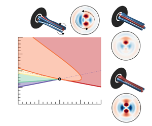
4.3. Fixed distance between jets and variable velocity ratio $\delta _u$

In the following, we focus on the influence of the velocity ratio  $\delta _u$ between jets for fixed jet distances $L$. Figure 17 displays the neutral curve of stability for jet distances (a) $L=0.5$ and (b) $L=1$. One may observe that the primary bifurcation is not always associated with the mode $S_1$ as is the case for $\delta _u=0$. For sufficiently large velocity ratios, the primary instability leads to a non-axisymmetric steady state with a double helix, corresponding to the unstable mode $S_2$. As can be appreciated in figure 9(b), for small values of $\delta _u$, the mode $S_1$ expands downstream over a relatively large area, having a higher activity than mode $S_2$, which is confined to the recirculation region. As the ratio between velocities is increased, as observed in figure 9(a), mode $S_2$ enlarges and resembles mode $S_1$, controlling the instability mechanism for large values of $\delta _u$. Another interesting feature, which could motivate a control strategy, is the occurrence of vertical asymptotes. This sudden change in the critical Reynolds number is due to the retraction, disappearance of the recirculation bubble and the formation of a new recirculating flow region, aspects that have been covered in § 3. For $L=0.5$, this sudden change occurs for $\delta _u \approx 0.25$, and for higher values of $\delta _u$ the critical Reynolds number is around twice larger than the one of the annular jet ( $\delta _u=0$). The case of jet distance $L=1$ was discussed in § 3. The sudden change in the stability of the branch $S_1$ occurs in the range $\delta _u \in [0.25,0.5]$. Within this narrow interval, the primary branch of instability is the $F_1$. At around $\delta _u=0.4$, the primary bifurcation is again the branch $S_1$, which becomes secondary at around $\delta _u \approx 0.8$ in favour of the branch $S_2$. In figure 17 we have highlighted the codimension two point interaction between the $S_1-S_2$ modes, which will be analysed in detail in § 5. Around this point, we can observe the largest ratio ( ${Re_c|_{\delta _u\neq 0}}/{Re_c|_{\delta _u=0}}$) between the value of the critical Reynolds number of the primary instability for a concentric jet configuration ( $\delta _u \neq 0$) and the annular jet problem ( $\delta _u=0$).

Figure 17. Linear stability boundaries for the concentric jets (a)  $L = 0.5$ and (b) $L = 1$. Same legend as figure 13.
4.4. Fixed velocity ratio $\delta _u$ and variable distance between jets

Figure 18 compares the results obtained for a constant velocity ratio when varying the distance between jets. As observed before, the increase of the distance between the jets has a de-stabilising effect. The largest critical Reynolds number is found at  $\delta _u=0$, and the critical Reynolds number decreases with the duct wall length $L$ between the jet streams. The points of codimension two are highlighted in figure 18. We can appreciate that the interaction between the branch $S_1$ and $S_2$ happens for every velocity ratio $\delta _u$ explored, and it is the mode interaction associated with the smallest distance between jets. Additionally, for a velocity ratio $\delta _u=0.5$ there exist two points where the branches of the linear modes $S_1$ and $F_1$ intersect. Another feature of the neutral curves is the existence of turning points, which are associated with the existence of saddle-node bifurcations of the axisymmetric steady state, addressed in § 3. The saddle-node bifurcations of the steady state induce the existence of regions in the neutral curves with a tongue shape. These saddle-node bifurcations are also responsible for the formation of the vertical asymptotes observed in figure 17. Finally, it is of interest the transition of the modes $S_1$ and $S_2$, which induce the symmetry breaking of the axisymmetric steady state to slow low frequency spiralling structures. These modes have been identified for $\delta _u=0.5$ for $m=1$, $\delta _u=1$ for $m=2$ and $\delta _u=2$ for both $m=1$ and $m=2$. As it will be clarified in § 5, these oscillations issue from the nonlinear interaction of modes, emerging simultaneously for a specific Reynolds number, and changing their position as the most unstable global mode of the flow.

Figure 18. Neutral lines of the four modes found by studying the configuration of two concentric jets and fixing the velocity ratio; (a,b)  $\delta _u =0.5$, (c,d) $\delta _u = 1$, (e, f) $\delta _u = 2$. Black lines: modes with $m=1$, red lines: modes with $m=2$. Straight lines: steady modes, dashed lines: unsteady modes. The discontinuity points, i.e. the points where the second most unstable mode (of a given type) becomes the most unstable, are highlighted with square markers.
5. Mode interaction between two steady states. Resonance 1 : 2
5.1. Normal form, basic solutions and their properties
The linear diagrams of § 4 have shown the existence of the mode interaction between the modes  $S_1$ and $S_2$. It corresponds roughly to the mode interaction that occurs at the largest critical Reynolds number for any value of $L$ herein explored. In this section, we analyse the dynamics near the $S_1:S_2$ organising centre. We perform a normal form reduction, which allows us to predict non-axisymmetric steady, periodic, quasiperiodic and heteroclinic cycles between non-axisymmetric states.
The mode interaction that is herein analysed corresponds to a steady–steady bifurcation with  $O(2)$ symmetry and with strong resonance 1 : 2. Such a bifurcation scenario has been extensively studied in the past by Dangelmayr (Reference Dangelmayr1986), Jones & Proctor (Reference Jones and Proctor1987), Porter & Knobloch (Reference Porter and Knobloch2001), Armbruster et al. (Reference Armbruster, Guckenheimer and Holmes1988) and for the reflection symmetry-breaking case (SO(2)) by Porter & Knobloch (Reference Porter and Knobloch2005). In order to unravel the existence and the stability of the nonlinear states near the codimension two point, let us write the flow field as
 \begin{equation} \boldsymbol{q} =
\boldsymbol{Q}_0 + {Re} [ r_1(\tau) {\rm e}^{{\rm i}
\phi_1(\tau)} {\rm e}^{-{\rm i}\theta}
\hat{\boldsymbol{q}}_{s,1} ] + {Re} [ r_2(\tau)
{\rm e}^{{\rm i} \phi_2(\tau)} {\rm e}^{{-}2{\rm i} \theta}
\hat{\boldsymbol{q}}_{s,2} ],
\end{equation}
\begin{equation} \boldsymbol{q} =
\boldsymbol{Q}_0 + {Re} [ r_1(\tau) {\rm e}^{{\rm i}
\phi_1(\tau)} {\rm e}^{-{\rm i}\theta}
\hat{\boldsymbol{q}}_{s,1} ] + {Re} [ r_2(\tau)
{\rm e}^{{\rm i} \phi_2(\tau)} {\rm e}^{{-}2{\rm i} \theta}
\hat{\boldsymbol{q}}_{s,2} ],
\end{equation}
in polar coordinates for the complex amplitudes  $z_1 = r_1 \textrm {e}^{\mathrm {i} \phi _1}$ and $z_2 = r_2 \textrm {e}^{\mathrm {i} \phi _2}$ where $r_j$ and $\phi _j$ for $j=1,2$ are the amplitude and phase of the symmetry-breaking modes $m=1$ and $m=2$, respectively. The complex-amplitude normal form (2.13) is expressed in this reduced polar notation as follows:
 $$\begin{gather} \dot{r}_{1} = e_3 r_{1} r_{2} \cos(\chi) + r_{1} ( \lambda_{(s,1)} + c_{(1,1)} r_{1}^2 + c_{(1,2)} r_{2}^2 ), \end{gather}$$
 $$\begin{gather}\dot{r}_{2} = e_4 r_{1}^2 \cos(\chi) + r_{2} ( \lambda_{(s,2)} + c_{(2,1)} r_{1}^2 + c_{(2,2)} r_{2}^2 ), \end{gather}$$
 $$\begin{gather}\dot{\chi} ={-} \left( 2 e_3 r_{2} + e_4 \frac{r_{1}^2}{r_{2}} \right) \sin(\chi), \end{gather}$$
where the phase  $\chi = \phi _2 - 2\phi _1$ is coupled to the amplitudes $r_1$ and $r_2$ because of the existence of the 1 : 2 resonance. The individual phases evolve as
 \begin{equation} \left.\begin{gathered} \dot{\phi}_1 = e_3 r_2 \sin(\chi), \\ \dot{\phi}_2 ={-} e_4 \frac{r_1^2}{r_2} \sin(\chi). \end{gathered}\right\} \end{equation}
Before proceeding to the analysis of the basic solutions of (5.2), we can simplify these equations by the rescaling
 \begin{equation} \left( \frac{r_1}{|e_3 e_4|^{1/2}}, \frac{r_2}{e_3} \right) \to (r_1,r_2), \end{equation}
which yields the following equivalent system:
 $$\begin{gather} \dot{r}_{1} = r_{1} r_{2} \cos(\chi) + r_{1} ( \lambda_{(s,1)} + c_{11} r_{1}^2 + c_{12} r_{2}^2 ), \end{gather}$$
 $$\begin{gather}\dot{r}_{2} = s r_{1}^2 \cos(\chi) + r_{2} ( \lambda_{(s,2)} + c_{21} r_{1}^2 + c_{22} r_{2}^2 ), \end{gather}$$
 $$\begin{gather}\dot{\chi} ={-} \frac{1}{r_2} ( 2 r_{2}^2 + s r_1^2) \sin(\chi), \end{gather}$$
where the coefficients
 \begin{align} s = \text{sign}(e_3 e_4), \quad c_{11} = \frac{c_{(1,1)}}{|e_3 e_4|}, \quad c_{12} = \frac{c_{(1,2)}}{e_3^2}, \quad c_{21} = \frac{c_{(2,1)}}{|e_3 e_4|}, \quad c_{22} = \frac{c_{(2,2)}}{e_3^2}. \end{align}
Finally, we consider a third normal form equivalent to the previous ones but which removes the singularity of (5.2) and (5.5) when  $r_2 = 0$. Standing waves ( $\sin \chi = 0$) naturally encounter this type of artificial singularity, which manifests in (5.5) as an instantaneous jump from one standing subspace to the other by a ${\rm \pi}$-translation. This is the case of the heteroclinic cycles, previously studied by Armbruster et al. (Reference Armbruster, Guckenheimer and Holmes1988) and Porter & Knobloch (Reference Porter and Knobloch2001). The third normal form, which we shall refer to as the reduced Cartesian normal form, takes advantage of the simple transformation $x=r_2 \cos (\chi )$, $y=r_2 \sin (\chi )$ (Porter & Knobloch Reference Porter and Knobloch2005)
 $$\begin{gather} \dot{r}_{1} = r_{1} ( \lambda_{(s,1)} + c_{11} r_{1}^2 + c_{12} (x^2+y^2) + x ), \end{gather}$$
 $$\begin{gather}\dot{x} = s r_{1}^2 + 2 y^2 + x( \lambda_{(s,2)} + c_{21} r_{1}^2 + c_{22} (x^2+y^2) ), \end{gather}$$
 $$\begin{gather}\dot{y} ={-} 2 xy + y ( \lambda_{(s,2)} + c_{21} r_{1}^2 + c_{22} (x^2+y^2) ). \end{gather}$$
In this final representation, standing wave solutions are contained within the invariant plane  $y=0$, and due to the invariance of (5.7) under the reflection $y \mapsto -y$, one can restrict attention, without loss of generality, to solutions with $y \geq 0$, cf. Porter & Knobloch (Reference Porter and Knobloch2001).
The system (5.5) possess four types of fixed points, which are listed in table 1.
Table 1. Definition of the fixed points of the reduced polar normal form (5.5);  $\sigma _{\pm }$ is defined in (5.8), the polynomial $P_{MM}$ is defined in (5.10) and $\varSigma _{TW} \equiv 4 c_{11} + 2 (c_{12} + c_{21}) + c_{22}$.

First, the axisymmetric steady state (O) is represented by  $(r_1,r_2) = (0,0)$, so it is the trivial steady state of the normal form. The second steady state is what it is denoted as the pure mode (P). In the original coordinates, it corresponds to the symmetry-breaking structure associated with the mode $S_2$. This state bifurcates from the axisymmetric steady state (O) when $\lambda _{(s,2)} = 0$. The third fixed point is the mixed-mode state (MM), which is listed in table 1. It corresponds to the reflection symmetry preserving state associated with the mode $S_1$. It may bifurcate directly from the trivial steady state O, when $\lambda _{(s,1)} = 0$ or from P whenever $\sigma _{+} = 0$ or $\sigma _{-} = 0$, where $\sigma _{\pm }$ is defined as
 \begin{equation} \sigma_{{\pm}} \equiv \lambda_{(s,1)} - \frac{-\lambda_{(s,2)} c_{12}}{c_{22}} \pm \sqrt{\frac{-\lambda_{(s,2)}}{c_{22}}} . \end{equation}
The representation in the reduced polar form is
 \begin{equation} r_{1,MM} ={-} \frac{ \lambda_{(s,1)} \pm r_{2,MM} + c_{12} r_{2,MM}^2 }{c_{11}}, \quad \cos(\chi_{MM}) ={\pm} 1, \end{equation}
and the condition  ${P}_{{MM}}(r_{2,MM} \cos (\chi _{MM})) = 0$, where ${P}_{{MM}}$ is defined as
 \begin{align} {P}_{{MM}}(x) \equiv s \mu_1 + (s + c_{21} \lambda_{(s,1)} - c_{(1,1)} \lambda_{(s,2)}) x + (c_{21} + s c_{12}) x^2 + (c_{12}c_{21} - c_{11}c_{22})x^3. \end{align}
Finally, the fourth fixed point of the system represents travelling waves (TW). It is surprising that the interaction between two steady states causes a time-periodic solution. The travelling wave emerges from MM in a parity-breaking pitchfork bifurcation that breaks the reflection symmetry when  $\cos (\chi _{TW}) = \pm 1$. The TW drifts at a steady rotation rate $\omega _{TW}$ along the group orbit, i.e. the phases $\dot {\phi }_1 = r_{2,TW} \sin (\chi _{TW})$ and $\dot {\phi }_2 = -s ({r_{1,TW}^2}/{r_{2,TW}}) \sin (\chi _{TW})$ are non-null.
Mixed modes and travelling waves may further bifurcate into standing waves (SW) and modulated travelling waves (MTW), respectively. These are generic features of the 1 : 2 resonance for small values of  $\lambda _{(s,1)}$ and $\lambda _{(s,2)}$, when $s = -1$. In the original coordinates, SW are periodic solutions, whereas MTW are quasiperiodic. Standing waves emerge via a Hopf bifurcation from MM when the conditions ${P}_{{SW}} (r_{2,MM} \cos (\chi _{MM}) ) > 0$ for
 \begin{equation} {P}_{{SW}} (x) \equiv (2 c_{22} x^3 - s r_1^2) c_{11} - (2 c_{12} x + 1)(c_{21}x + s)x, \end{equation}
and the one listed in table 2 are satisfied. The MTW are created when a torus bifurcation happens on the travelling wave branch when the conditions listed in table 2 are satisfied.
Table 2. Definition of the limit cycles of the reduced polar normal form (5.5).

Another remarkable feature of (5.2) is the existence of robust heteroclinic cycles that are asymptotically stable. When  $s = -1$, there are open sets of parameters where the reduced polar normal form exhibits structurally stable connections between ${\rm \pi}$-translations on the circle of pure modes, cf. Armbruster et al. (Reference Armbruster, Guckenheimer and Holmes1988). These structures are robust and have been observed in a large variety of systems, (Palacios et al. Reference Palacios, Gunaratne, Gorman and Robbins1997; Mercader, Prat & Knobloch Reference Mercader, Prat and Knobloch2002; Nore et al. Reference Nore, Tuckerman, Daube and Xin2003; Mariano & Stazi Reference Mariano and Stazi2005; Nore, Moisy & Quartier Reference Nore, Moisy and Quartier2005). In addition to these robust heteroclinic cycles connecting pure modes, there exist more complex limit cycles connecting O, P, MM and SW, cf. Porter & Knobloch (Reference Porter and Knobloch2001). These cycles are located for larger values of $\lambda _{(s,1)}$ and $\lambda _{(s,2)}$, with a possibly chaotic dynamics (Shilnikov type). In this study, we have not identified any of these. Finally, a summary of the basic solutions and the bifurcation path is sketched in figure 19.

Figure 19. Schematic representation of the basic solutions of (5.2) and their bifurcation path.
5.2. Results of the steady–steady 1 : 2 mode interaction
Section 4.4 reported the location of mode interaction points for discrete values of the velocity ratio  $\delta _u$. The location of the mode interaction between $S_1$ and $S_2$ is depicted in figure 20. It shows that the mode switching between the modes $S_1$ and $S_2$ is indeed stationary only for $\delta _u < 1.5$ and $L < 1.3$. For larger values of the velocity ratio and the jet distance, the interaction is not purely stationary; at least one of the linear modes oscillates with a slow frequency. It implies that the mode selection for large velocity ratios near the codimension two points is similar to the one reported by Meliga et al. (Reference Meliga, Gallaire and Chomaz2012) for swirling jets. However, even when the two primary bifurcations are non-oscillating ( $S_1$ and $S_2$), the 1 : 2 resonance of the azimuthal wavenumbers induces a slow frequency, what we denote as travelling wave solutions.

Figure 20. Evolution of the codimension two interaction  $S_1-S_2$ in the space of parameters $({Re},L,\delta _u)$. Grey points denote the points that were computed and the red point denotes the transition from steady to unsteady with low frequency as reported in § 4.4.
We consider the bifurcation sequence for  $\delta _u = 1.0$ and $L=1.15$, which is qualitatively similar to transitions in the range $0.5 < \delta _u < 1.5$, near the codimension two points, which are depicted in figure 20. At the codimension two points for $\delta _u < 0.5$, at least one of the two bifurcations is sub-critical and a normal form reduction up to fifth order is necessary. Subcritical transition was also noticed for a distance between jets $L=0.1$ by Canton et al. (Reference Canton, Auteri and Carini2017), who reported high levels of the linear gain associated with transient growth mechanisms. This last case is outside of the scope of the present manuscript. Figure 21 displays the phase portrait of the stable attractors near the $S_1:S_2$ interaction. For values of $\delta _u > 1.0$, the axisymmetric steady state loses its axisymmetry leading to a new steady state with symmetry $m=2$, herein denoted as pure mode (P). A reconstruction of the perturbative component of the flow field of such a state is performed at the bottom right of figure 21, which shows that the state P possesses two orthogonal planes of symmetry. Near the codimension two point, for values of the velocity ratio $\delta _u < 1.1$, the state P is only observable, that is nonlinearly stable, within a small interval with respect to the Reynolds number. For larger values of the velocity ratio, the state P remains stable within the analysed interval of Reynolds numbers. For values of the velocity ratio $\delta _u < 1.0$, the bifurcation diagram is more complex. Figure 22 displays the bifurcation diagram of the fixed-point solutions of (5.7) on the left diagram and the full set of solutions of the normal form in the right diagram. The axisymmetric steady state first bifurcates towards a mixed-mode solution, which is the solution in the $y=0$ plane for the right diagram of figure 22. A solution with a non-symmetric wake has been reconstructed in figure 21. The mixed-mode solution is only stable within a small interval of the Reynolds number. A secondary bifurcation, denoted $\textrm {Bif}_{MM-TW}$, gives rise to a slowly rotating wave of the wake. The TW and the MM solutions are identical at the bifurcation point. The phase speed is zero at the bifurcation, thus this is not a Hopf bifurcation. It corresponds to a drift instability that breaks the azimuthal symmetry, i.e. it starts to slowly drift. This unusual feature, that travelling waves bifurcate from a steady solution at a steady bifurcation, is a generic feature of the 1 : 2 resonance. A reconstruction of the travelling wave solution is depicted on the top of figure 21. It corresponds to the line with non-zero $y$ component in the right diagram of figure 22. The TW solution loses its stability in a tertiary bifurcation, denoted as Bif $_{TW-MTW}$. It conforms to a Hopf bifurcation of the TW solution, which gives birth to a quasi-periodic solution named the modulated travelling wave (MTW). A representation of this kind of solution in Cartesian coordinates $(r_1,x,y)$ is depicted in figure 22(b).

Figure 21. Parametric portrait at the codimension two point  $S_1:S_2$ for parameter values $(L,\delta _u) = (1.15,1.0)$. The colour-shaded areas corresponds to the regions in the parameter space where a given solution is attracting, e.g. the green-shaded area is the region where TW is the attracting solution. Solid lines indicate codimension-one bifurcations, dashed lines indicate when $\lambda _{(s,2)} = 0$ (P) and $\lambda _{(s,1)} = 0$ (MM), a grey marker denotes the codimension-two point. The visualisations of blue and red surfaces in the isometric views represent the respective positive and negative isocontour values of the perturbative axial velocity indicated in the figure.

Figure 22. Bifurcation diagram with respect to the Reynolds number for  $L = 1.15$ and $\delta _u = 0.8$. The (a) diagram reports the evolution of $r_2$ for the fixed-point solutions of the normal form. The (b) diagram displays the bifurcation diagram in the Cartesian coordinates. Solid lines and dashed lines denote stable attractors and unstable attractors, respectively.
Eventually, the modulated travelling wave experiences a global bifurcation. That occurs when the periodic MTW solution, in  $(r_1,x,y)$ coordinates, nearly intersects the invariant $r_1=0$ and $y=0$ planes. The transition sequence is represented in figure 22(b) in Cartesian coordinates ( $r_1,x,y$). The amplitude of the MTW limit cycle increases until the MTW arising at the tertiary bifurcation Bif $_{TW-MTW}$ are destroyed by meeting a heteroclinic cycle at Bif $_{MTW-Ht}$. The locus of Bif $_{MTW-Ht}$ is reported in figure 21 and in good agreement with Armbruster et al. (Reference Armbruster, Guckenheimer and Holmes1988). The conditions for the existence of the heteroclinic cycles are: $\lambda _{(s,1)} > 0$, $\lambda _{(s,2)} > 0$, $c_{22} < 0$. When $\sigma _{-}$ becomes negative, the cycle is attracting and robust heteroclinic cycles are observed. It is destroyed when $\sigma _{+}$ becomes negative, in that case the pure modes are no longer saddles, which breaks the heteroclinic connection. Figure 23 displays the instantaneous fluctuation field from a heteroclinic orbit connecting P and its conjugate solution P’, which is obtained by a rotation of ${\rm \pi} /2$, for parameter values ${Re} = 200$ and $\delta _u = 0.8$. The dynamics of the cycle takes place in two phases. Figure 23 depicts the motion of the coherent structure associated with the heteroclinic cycle. Starting from the conjugated pure mode $\textrm {P}'$, the cycle leaves the point (a), located in the vicinity of $\textrm {P}'$, along the unstable eigenvector $y$, which is the stable direction of P. The first phase consists in a rapid rotation by ${\rm \pi} /2$ of the wake, it corresponds to the sequence a-b-c-d-e displayed in figure 23. Then it is followed by a slow approach following the direction $y$ and departure from the pure mode state P along the direction $r_1$. The second phase consists in a rapid horizontal motion of the wake, which is an evolution from P to $\textrm {P}'$ that takes place by the breaking of the reflectional symmetry with respect to the vertical axis; it constitutes the sequence e-f-g-h-i-a. Please note that equivalent motions are also possible. The first phase of rapid counter-clockwise rotation by ${\rm \pi} /2$ can be performed in the opposite sense. It corresponds to a motion in Cartesian coordinates along the plane $r_1$ along negative values of $y$. The sequence e-f-g-h-i-a can be replaced by a horizontal movement in the opposite sense, which adjusts to connect the plane $y=0$ corresponding to negative values of $r_1$.

Figure 23. Heteroclinic cycle solution for parameter values  ${Re}=200$, $\delta _u = 0.8$. The top and bottom image sequences along the heteroclinic cycle show (from left to right) an axial slice plane at $z=1$ of the instantaneous fluctuations of the axial velocity of the flow field as viewed from downstream, along with a three-dimensional isometric view (d on the top and g on the bottom).The middle diagram displays the heteroclinic cycle in the coordinates ( $r_1,x,y$).
6. Discussion and conclusions
The current study provides a complete description of the configuration consisting of two coaxial jets, broadly found in industrial processes, covering a wide range of applications such as noise reduction, mixing enhancement or combustion control. The numerical procedure herein employed has been validated with the existing literature in the case of the stability analysis (see Appendix B for a detailed overview). A large region of the parameter space is explored  $(\delta _u, L) \in ([0,2], [0.5,4.5])$, substantially expanding the work of Canton et al. (Reference Canton, Auteri and Carini2017).
Section 3 provides an analysis of the basic properties of the steady state, such as the topology of the flow and its variations in terms of the three parameters  $(Re,L,\delta _u)$. It also highlights the existence of multiple steady states, as a result of a series of saddle-node bifurcations, and the connection between the bifurcation and flow topology. Highlighting, nonetheless, that changes in the topology are not a direct consequence of a saddle-node bifurcation. The linear stability analysis performed in § 4 reveals the existence of two unstable steady modes: $S_1$ and $S_2$, which are mostly located within the recirculation bubble, and two unsteady ones: $F_1$ and $F_2$, which are also produced within the recirculating region of the flow, but they are convected downstream, while experiencing substantial amplification. In addition, in § 4, we briefly discuss the consequences of the retraction and eventual disappearance of the recirculation bubble and the formation of a new recirculating flow region, aspects that have been covered in § 3, in terms of the sudden changes in the critical Reynolds number. Subsequently, the critical Reynolds number is determined for a wide range of inner-to-outer velocity rations and duct wall lengths. An increase of the velocity ratio has an overall stabilising effect, and it leads to the swap from mode $S_1$, characterised with one symmetry plane, to mode $S_2$ that possesses two symmetry planes. Afterwards, the effect of the distance $L$ between jets is analysed. The primary effect of increasing this distance is a decrease in the critical Reynolds number for all values of $\delta _u$ investigated.
Section 5 analyses the mode interaction between two symmetry-breaking modes with azimuthal wavenumbers  $m=1$ and $m=2$. The unfolding of the codimension-two bifurcation reveals the presence of unsteadiness as a result of the resonant 1 : 2 interaction between the two steady modes. The codimension-two point is located at a velocity ratio $\delta _u = 1.0$ and distance between jets of $L=1.15$, a situation that it is qualitatively equivalent to transitions found in the range $0.5<\delta _u<1.5$. For values lower than $\delta _u=1.0$, the bifurcation diagram exhibits an intricate path. First, a MM solution emerges, which displays a non-symmetric wake. The MM solution is only stable for a small range of the Reynolds number. Subsequently, a slowly rotating wake is triggered in the form of a TW. This unusual feature, an unsteady state emerging from a steady state, corresponds to a drift instability commonly found at 1 : 2 resonance. Then, the TW solution encounters a Hopf bifurcation, developing a quasi-periodic solution in the form of a MTW. Finally, the MTW solution undergoes a global bifurcation meeting a heteroclinic cycle. This heteroclinic orbit links the solution P with its conjugate solution $\textrm {P}'$, spinning the wake from $\textrm {P}'$ to P, and moving it horizontally from P to $\textrm {P}'$. On the other hand, for values higher than $\delta _u=1.0$, a non-axisymmetric steady state emerges as a pure mode P with two orthogonal planes of symmetry. If the transition happens for values of the velocity ratio close to unity, a further increase in the velocity ratio rapidly leads to the heteroclinic cycle.
Physical realisations of the 1 : 2 mode interaction have been observed by Mercader et al. (Reference Mercader, Prat and Knobloch2002) and Nore et al. (Reference Nore, Tuckerman, Daube and Xin2003, Reference Nore, Moisy and Quartier2005) for confined flow configurations. However, to the authors’ knowledge, this is the first time that a robust heteroclinic cycle resulting from this type of 1 : 2 interaction is reported in the literature for an external flow configuration, as is the coaxial jet configuration.
Funding
A.C., J.A.M. and S.L.C. acknowledge the grant PID2020-114173RB-I00 funded by MCIN/AEI/10.13039/501100011033. S.L.C., J.A.M. and A.C. acknowledge the support of Comunidad de Madrid through the call Research Grants for Young Investigators from Universidad Politécnica de Madrid. A.C. also acknowledges the support of Universidad Politécnica de Madrid, under the programme ‘Programa Propio’.
Declaration of interests
The authors declare no conflict of interest.
Appendix A. Normal form reduction
In this section we provide a detailed explanation of the normal form reduction to obtain the coefficients of (2.13), we define the terms of the compact notation of the governing equations (2.4), which is reminded here, for the sake of conciseness
 \begin{equation} \boldsymbol{B} \frac{\partial \boldsymbol{Q}}{\partial t} = \boldsymbol{F}(\boldsymbol{Q}, \boldsymbol{\eta}) \equiv \boldsymbol{L} \boldsymbol{Q} + \boldsymbol{N}(\boldsymbol{Q},\boldsymbol{Q}) + \boldsymbol{G} (\boldsymbol{Q},\boldsymbol{\eta}). \end{equation}
The nonlinear convective operator  $\boldsymbol{N}(\boldsymbol{Q}_1,\boldsymbol{Q}_2) = \boldsymbol{U}_1 \boldsymbol {\cdot } \boldsymbol {\nabla } \boldsymbol{U}_2$ accounts for the quadratic interaction on the state variable. The linear operator on the state variable is $\boldsymbol{L} \boldsymbol{Q} = [\boldsymbol {\nabla } P, \boldsymbol {\nabla } \boldsymbol {\cdot } \boldsymbol{U} ]^\textrm {T}$. The remaining term accounts for the linear variations in the state variable and the parameter vector. It is defined as $\boldsymbol{G}(\boldsymbol{Q},\boldsymbol {\eta }) = \boldsymbol{G}(\boldsymbol{Q},[\eta _1,0]^\textrm {T}) + \boldsymbol{G}(\boldsymbol{Q},[0,\eta _2]^\textrm {T})$ where $\boldsymbol{G}(\boldsymbol{Q},[\eta _1,0]^\textrm {T}) = \eta _1 \boldsymbol {\nabla } \boldsymbol {\cdot }(\boldsymbol {\nabla } \boldsymbol{U} + \boldsymbol {\nabla } \boldsymbol{U}^T)$ and $\boldsymbol{G}(\boldsymbol{Q},[0,\eta _2]^\textrm {T})$. The former operator shows the dependency on the parameter $\eta _1$, which accounts for the viscous effects. The latter operator depends on the parameter $\eta _2$, which accounts for the velocity ratio between jets and it is used to impose the boundary condition $\boldsymbol{U} = (0, \eta _2 \tanh (b_i (1 - 2r)) , 0)$ on $\varGamma _{in,i}$. In addition, we consider the following splitting of the parameters $\boldsymbol {\eta } = \boldsymbol {\eta }_c + \Delta \boldsymbol {\eta }$. Here, $\boldsymbol {\eta }_c$ denotes the critical parameters $\boldsymbol {\eta }_c \equiv [Re_c^{-1}, \delta _{u,c}]^\textrm {T}$ attained when the spectra of the Jacobian operator possess at least an eigenvalue whose real part is zero. The distance in the parameter space to the threshold is represented by $\Delta \boldsymbol {\eta } = [Re_c^{-1} - Re^{-1}, \delta _{u,c} - \delta _u]^\textrm {T}$.
A.1. Multiple scales ansatz
The multiple scales expansion of the solution  $\boldsymbol{q}$ of (2.4) is
 \begin{equation} \boldsymbol{q}(t,\tau) = \boldsymbol{Q}_0 + \varepsilon \boldsymbol{q}_{(\varepsilon)}(t,\tau) + \varepsilon^2 \boldsymbol{q}_{(\varepsilon^2)}(t,\tau) + O(\varepsilon^3), \end{equation}
where  $\varepsilon \ll 1$ is a small parameter. The distance in the parameter space to the critical point $\Delta \boldsymbol {\eta } = [Re_c^{-1} - Re^{-1}, \delta _{u,c} - \delta _u]^\textrm {T}$ is assumed to be of second order, i.e. $\Delta {\eta }_i = O(\varepsilon ^2)$ for $i=1,2$. The expansion (A2) considers a two scale expansion of the original time $t \mapsto t + \varepsilon ^2 \tau$. A fast time scale $t$ and a slow time scale of the evolution of the amplitudes $z_i(\tau )$ in (A2), for $i=1,2$. Note that the expansion of the left-hand side (2.4) up to third order is as follows:
 \begin{equation} \varepsilon \boldsymbol{B} \frac{\partial \boldsymbol{q}_{(\varepsilon)}} {\partial t} + \varepsilon^2 \boldsymbol{B} \frac{\partial \boldsymbol{q}_{(\varepsilon^2)}} {\partial t} + \varepsilon^3 \left[ \boldsymbol{B} \frac{\partial \boldsymbol{q}_{(\varepsilon^3)}} {\partial t} + \boldsymbol{B} \frac{\partial \boldsymbol{q}_{(\varepsilon)}} {\partial \tau} \right], \end{equation}
and the right-hand side respectively,
 \begin{equation} \boldsymbol{F} (\boldsymbol{q}, \boldsymbol{\eta}) = \boldsymbol{F}_{(0)} + \varepsilon \boldsymbol{F}_{(\varepsilon)} + \varepsilon^2 \boldsymbol{F}_{(\varepsilon^2)} + \varepsilon^3 \boldsymbol{F}_{(\varepsilon^3)}. \end{equation}
The expansion (A4) will be detailed at each order.
A.1.1. Order $\varepsilon ^0$

The zeroth order  $\boldsymbol{Q}_0$ of the multiple scales expansion (A2) is the steady state of the governing equations evaluated at the threshold of instability, i.e. $\boldsymbol {\eta } = \boldsymbol {\eta }_c$,
 \begin{equation} \boldsymbol{0} = \boldsymbol{F} (\boldsymbol{Q}_0, \boldsymbol{\eta}_c). \end{equation}
A.1.2. Order $\varepsilon ^1$

The first order  $\boldsymbol{q}_{(\varepsilon )}(t,\tau )$ of the multiple scales expansion of (A2) is composed of the eigenmodes of the linearised system
 \begin{equation} \boldsymbol{q}_{(\varepsilon)}(t,\tau) \equiv ( z_1(\tau) {\rm e}^{-\mathrm{i} m_1 \theta} \hat{\boldsymbol{q}}_{1} + z_2(\tau) {\rm e}^{\mathrm{i} -m_2 \theta} \hat{\boldsymbol{q}}_{2} + \text{c.c.} ). \end{equation}
In our case,  $m_1 = 1$ and $m_2 = 2$. Each term $\hat {\boldsymbol{q}}_\ell$ of the first-order expansion (A6) is a solution of the following linear equation:
 \begin{equation} \boldsymbol{J}_{(\omega_\ell, m_\ell)} \hat{\boldsymbol{q}}_{\ell} \equiv \left({\rm i}\omega_\ell \boldsymbol{B} - \frac{\partial \boldsymbol{F}}{\partial \boldsymbol{q} }|_{\boldsymbol{q} = \boldsymbol{Q}_0, \boldsymbol{\eta} = \boldsymbol{\eta}_c} \right) \hat{\boldsymbol{q}}_{\ell} = 0, \end{equation}
where  ${\partial \boldsymbol{F}}/{\partial \boldsymbol{q} }|_{\boldsymbol{q} = \boldsymbol{Q}_0, \boldsymbol {\eta } = \boldsymbol {\eta }_c} \hat {\boldsymbol{q}}_{\ell } = \boldsymbol{L}_{m_\ell } \hat {\boldsymbol{q}}_{\ell } + \boldsymbol{N}_{m_\ell }(\boldsymbol{Q}_0, \hat {\boldsymbol{q}}_{\ell } ) + \boldsymbol{N}_{m_\ell }(\hat {\boldsymbol{q}}_{\ell }, \boldsymbol{Q}_0 )$. The subscript $m_\ell$ indicates the azimuthal wavenumber used for the evaluation of the operator.
A.1.3. Order $\varepsilon ^2$

The second-order expansion term  $\boldsymbol{q}_{(\varepsilon ^2)}(t,\tau )$ is determined from the resolution of a set of forced linear systems, where the forcing terms are evaluated from first- and zeroth-order terms. The expansion in terms of amplitudes $z_i(\tau )$ ( $i=1,2$) of $\boldsymbol{q}_{(\varepsilon ^2)}(t,\tau )$ is assessed from term-by-term identification of the forcing terms at the second order. Nonlinear second-order terms in $\varepsilon$ are
 \begin{align}
\boldsymbol{F}_{(\varepsilon^2)} & \equiv \displaystyle
\sum_{j,k=1}^2 ( z_j z_k
\boldsymbol{N}(\hat{\boldsymbol{q}}_j,\hat{\boldsymbol{q}}_k)
\exp({-\mathrm{i}(m_j+m_k)\theta}) + \text{c.c.} )
\nonumber\\ &\quad + \displaystyle \sum_{j,k=1}^2 (
z_j \bar{z}_k \boldsymbol{N}(\hat{\boldsymbol{q}}_j,
\bar{\hat{\boldsymbol{q}}}_k)
\exp({-\mathrm{i}(m_j-m_k)\theta}) + \text{c.c.} )
\nonumber\\ &\quad + \displaystyle \sum_{\ell=0}^2
\eta_\ell \boldsymbol{G}(\boldsymbol{Q}_0,
\boldsymbol{e}_\ell), \end{align}
\begin{align}
\boldsymbol{F}_{(\varepsilon^2)} & \equiv \displaystyle
\sum_{j,k=1}^2 ( z_j z_k
\boldsymbol{N}(\hat{\boldsymbol{q}}_j,\hat{\boldsymbol{q}}_k)
\exp({-\mathrm{i}(m_j+m_k)\theta}) + \text{c.c.} )
\nonumber\\ &\quad + \displaystyle \sum_{j,k=1}^2 (
z_j \bar{z}_k \boldsymbol{N}(\hat{\boldsymbol{q}}_j,
\bar{\hat{\boldsymbol{q}}}_k)
\exp({-\mathrm{i}(m_j-m_k)\theta}) + \text{c.c.} )
\nonumber\\ &\quad + \displaystyle \sum_{\ell=0}^2
\eta_\ell \boldsymbol{G}(\boldsymbol{Q}_0,
\boldsymbol{e}_\ell), \end{align}
where the terms proportional to  $z_j z_k$ are named $\hat {\boldsymbol{F}}_{(\epsilon ^2)}^{(z_j z_k)}$ and $\boldsymbol{e}_\ell$ is an element of the orthonormal basis of $\mathbb {R}^2$.
Then, we look for a second-order term expanded as follows:
 \begin{equation} \boldsymbol{q}_{(\varepsilon^2)} \equiv \displaystyle \sum_{\substack{j,k=1 \\ k\leqslant j}}^{2} ( z_j z_k \hat{\boldsymbol{q}}_{z_j z_k} + z_j \bar{z}_k \hat{\boldsymbol{q}}_{z_j \bar{z}_k} + \text{c.c.}) + \sum_{\ell=1}^2 \eta_\ell \boldsymbol{Q}_0^{(\eta_\ell)}. \end{equation}
Terms  $\hat {\boldsymbol{q}}_{z^2_j}$ are azimuthal harmonics of the flow. The terms $\hat {\boldsymbol{q}}_{z_j z_k}$ with $j \neq k$ are coupling terms, and $\hat {\boldsymbol{q}}_{|z_j|^2}$ are harmonic base flow modification terms. Finally, $\boldsymbol{Q}_0^{(\eta _\ell )}$ are base flow corrections due to a variation of the parameter $\eta _\ell$ from the critical point.
At this order, there exist two resonant terms, the terms proportional to  $\bar {z}_1 z_2$ and $z_1^2$, which are associated with the singular Jacobian $\boldsymbol{J}_{(0,m_k)}$ for $k=1,2$. To ensure the solvability of these terms, we must enforce compatibility conditions, i.e. the Fredholm alternative. The resonant terms are then determined from the resolution of the following set of bordered systems:
 \begin{equation} \begin{pmatrix}
\boldsymbol{J}_{(0,m_k)} & \hat{\boldsymbol{q}}_{k} \\
\hat{\boldsymbol{q}}_{k}^{{\dagger}} & 0 \end{pmatrix}
\begin{pmatrix}
\hat{\boldsymbol{q}}_{(\boldsymbol{z}^{(R)})} \\ e
\end{pmatrix} = \begin{pmatrix}
\hat{\boldsymbol{F}}^{(\boldsymbol{z}^{(R)})}_{(\varepsilon^2)}
\\ 0 \end{pmatrix}, \quad \boldsymbol{z}^{(R)} \in
[\bar{z}_1 z_2, z_1^2]^{\rm T},
\end{equation}
\begin{equation} \begin{pmatrix}
\boldsymbol{J}_{(0,m_k)} & \hat{\boldsymbol{q}}_{k} \\
\hat{\boldsymbol{q}}_{k}^{{\dagger}} & 0 \end{pmatrix}
\begin{pmatrix}
\hat{\boldsymbol{q}}_{(\boldsymbol{z}^{(R)})} \\ e
\end{pmatrix} = \begin{pmatrix}
\hat{\boldsymbol{F}}^{(\boldsymbol{z}^{(R)})}_{(\varepsilon^2)}
\\ 0 \end{pmatrix}, \quad \boldsymbol{z}^{(R)} \in
[\bar{z}_1 z_2, z_1^2]^{\rm T},
\end{equation}
where  $e=e_3$ for $\boldsymbol{z}^{(R)} = \overline {z}_1 z_2$ and $e=e_4$ for $\boldsymbol{z}^{(R)} = z_1^2$. The non-resonant terms are computed by solving the following non-degenerated forced linear systems:
 \begin{equation} \boldsymbol{J}_{(0, m_j + m_k)} \hat{\boldsymbol{q}}_{z_j z_k} = \hat{\boldsymbol{F}}_{(\epsilon^2)}^{(z_j z_k)}, \end{equation}
and
 \begin{equation} \boldsymbol{J}_{(0,0)} \boldsymbol{Q}_0^{(\eta_\ell)} = \boldsymbol{G}(\boldsymbol{Q}_0, \boldsymbol{e}_\ell). \end{equation}
A.1.4. Order $\varepsilon ^3$

At third order, there exist six degenerate terms. In our case, we are not interested in solving for terms of third order, instead, we will determine the linear and cubic coefficients of the third-order normal form (2.13) from a set of compatibility conditions.
The linear terms  $\lambda _{(s,1)}$ and $\lambda _{s,2}$ and cubic terms $c_{(i,j)}$ for $i=1,2$ are determined as follows:
 \begin{equation} \lambda_{(s,1)} = \frac{\langle \hat{\boldsymbol{q}}_1^{{\dagger}}, \hat{\boldsymbol{F}}^{(z_1)}_{(\varepsilon^3)} \rangle}{\langle \hat{\boldsymbol{q}}_z^{{\dagger}}, \boldsymbol{B} \hat{\boldsymbol{q}}_z \rangle }, \quad \lambda_{(s,2)} = \frac{\langle \hat{\boldsymbol{q}}_2^{{\dagger}}, \hat{\boldsymbol{F}}^{(z_2)}_{(\varepsilon^3)} \rangle}{\langle \hat{\boldsymbol{q}}_2^{{\dagger}}, \boldsymbol{B} \hat{\boldsymbol{q}}_2 \rangle }, \quad{} c_{(i,j)} = \frac{\langle \hat{\boldsymbol{q}}_2^{{\dagger}}, \hat{\boldsymbol{F}}^{(z_i |z_j|^2)}_{(\varepsilon^3)} \rangle}{\langle \hat{\boldsymbol{q}}_i^{{\dagger}}, \boldsymbol{B} \hat{\boldsymbol{q}}_i \rangle }. \end{equation}
The forcing terms for the linear coefficient are
 \begin{equation}
\hat{\boldsymbol{F}}^{(z_j)}_{(\varepsilon^3)} \equiv
\sum_{\ell=1}^2 \eta_\ell ( [
\boldsymbol{N}(\hat{\boldsymbol{q}}_j,\boldsymbol{Q}_0^{(\eta_\ell))}
+
\boldsymbol{N}(\boldsymbol{Q}_0^{(\eta_\ell)},\hat{\boldsymbol{q}}_j) ] + \boldsymbol{G}(\hat{\boldsymbol{q}}_j,
\boldsymbol{e}_\ell)),
\end{equation}
\begin{equation}
\hat{\boldsymbol{F}}^{(z_j)}_{(\varepsilon^3)} \equiv
\sum_{\ell=1}^2 \eta_\ell ( [
\boldsymbol{N}(\hat{\boldsymbol{q}}_j,\boldsymbol{Q}_0^{(\eta_\ell))}
+
\boldsymbol{N}(\boldsymbol{Q}_0^{(\eta_\ell)},\hat{\boldsymbol{q}}_j) ] + \boldsymbol{G}(\hat{\boldsymbol{q}}_j,
\boldsymbol{e}_\ell)),
\end{equation}
which allows the decomposition of  $\lambda _{(s,\ell )} = \lambda _{(s,\ell ),{Re}} ({Re}^{-1}_c {Re}^{-1}) + \lambda _{(s,\ell ),{\delta _u}} (\delta _{u,c}- \delta _u)$ for $\ell = 1,2$.
The forcing terms for the cubic coefficients are
 \begin{align}
\hat{\boldsymbol{F}}^{({z}_j |z_k|^2)}_{(\varepsilon^3)} &
\equiv [
\boldsymbol{N}(\hat{\boldsymbol{q}}_j,\hat{\boldsymbol{q}}_{|z_k|^2})
+
\boldsymbol{N}(\hat{\boldsymbol{q}}_{|z_k|^2},\hat{\boldsymbol{q}}_j)
] \nonumber\\ &\quad + [
\boldsymbol{N}(\hat{\boldsymbol{q}}_{{-}k},\hat{\boldsymbol{q}}_{z_j
z_k}) +
\boldsymbol{N}(\hat{\boldsymbol{q}}_{j,k},\hat{\boldsymbol{q}}_{{-}k})
] \nonumber\\ &\quad + [
\boldsymbol{N}(\hat{\boldsymbol{q}}_{k},\hat{\boldsymbol{q}}_{z_j
\bar{z}_k}) + \boldsymbol{N}(\hat{\boldsymbol{q}}_{z_j
\bar{z}_k},\hat{\boldsymbol{q}}_{k}) ], \end{align}
\begin{align}
\hat{\boldsymbol{F}}^{({z}_j |z_k|^2)}_{(\varepsilon^3)} &
\equiv [
\boldsymbol{N}(\hat{\boldsymbol{q}}_j,\hat{\boldsymbol{q}}_{|z_k|^2})
+
\boldsymbol{N}(\hat{\boldsymbol{q}}_{|z_k|^2},\hat{\boldsymbol{q}}_j)
] \nonumber\\ &\quad + [
\boldsymbol{N}(\hat{\boldsymbol{q}}_{{-}k},\hat{\boldsymbol{q}}_{z_j
z_k}) +
\boldsymbol{N}(\hat{\boldsymbol{q}}_{j,k},\hat{\boldsymbol{q}}_{{-}k})
] \nonumber\\ &\quad + [
\boldsymbol{N}(\hat{\boldsymbol{q}}_{k},\hat{\boldsymbol{q}}_{z_j
\bar{z}_k}) + \boldsymbol{N}(\hat{\boldsymbol{q}}_{z_j
\bar{z}_k},\hat{\boldsymbol{q}}_{k}) ], \end{align}
if  $j \neq k$ and
 \begin{align}
\hat{\boldsymbol{F}}^{({z}_j |z_j|^2)}_{(\epsilon^3)} &
\equiv [
\boldsymbol{N}(\hat{\boldsymbol{q}}_j,\hat{\boldsymbol{q}}_{|z|_j^2})
+ \boldsymbol{N}(\hat{\boldsymbol{q}}_{|z|_j^2},
\hat{\boldsymbol{q}}_j) ] \nonumber\\ &\quad + [
\boldsymbol{N}(\hat{\boldsymbol{q}}_{{-}j},\hat{\boldsymbol{q}}_{z_j^2})
+
\boldsymbol{N}(\hat{\boldsymbol{q}}_{z^2_j},\hat{\boldsymbol{q}}_{{-}j})
], \end{align}
\begin{align}
\hat{\boldsymbol{F}}^{({z}_j |z_j|^2)}_{(\epsilon^3)} &
\equiv [
\boldsymbol{N}(\hat{\boldsymbol{q}}_j,\hat{\boldsymbol{q}}_{|z|_j^2})
+ \boldsymbol{N}(\hat{\boldsymbol{q}}_{|z|_j^2},
\hat{\boldsymbol{q}}_j) ] \nonumber\\ &\quad + [
\boldsymbol{N}(\hat{\boldsymbol{q}}_{{-}j},\hat{\boldsymbol{q}}_{z_j^2})
+
\boldsymbol{N}(\hat{\boldsymbol{q}}_{z^2_j},\hat{\boldsymbol{q}}_{{-}j})
], \end{align}
for the diagonal forcing terms.
Appendix B. Validation of the code – comparison with the literature
The calculations made in StabFem in the sections of the main manuscript are validated by comparing with leading global mode in the geometry proposed by Canton et al. (Reference Canton, Auteri and Carini2017). Moreover, the critical Reynolds number and associated frequency are also analysed. In the cited work, the authors use an analogous geometry with the following parameters:
(i) Radius of the inner jet
$R_{inner} = 0.5$.(ii) Diameter of the outer jet
$D = 0.4$.(iii) Distance between jets
$L = 0.1$.(iv) Ratio between velocities
$\delta _u = 1$.


The linear stability analysis has been carried out by imposing  $m = 0$, as done by Canton et al. (Reference Canton, Auteri and Carini2017), so the leading global mode will be axisymmetric. The critical Reynolds number $Re_c$ and the frequency $\omega$ of the leading global mode are compared in table 3. As seen, few differences can be found in the critical Reynolds number and the frequency. The relative error in the $Re_c$ calculation is $1.06\,\%$ and the one of the frequency is $0.17\,\%$.
Table 3. Comparison of  $Re_c$ and $\omega$ between previous work and the present one.

The global mode is now calculated using StabFem and compared with the one calculated by Canton et al. (Reference Canton, Auteri and Carini2017), as presented in figure 24. This mode can be found in figures 9, 10 and 11 in the cited paper. As can be seen, there are no substantial differences between the direct modes, both of them being a vortex street with their biggest amplitude situated 10 units downstream of the exit of the jets. The adjoint mode is concentrated within the nozzle, with its biggest amplitude situated on the sharp corners. There is no difference between the adjoint mode calculated with StabFem and the one in Canton et al. (Reference Canton, Auteri and Carini2017). Finally, the structural sensitivity is similar to the one computed by Canton et al. (Reference Canton, Auteri and Carini2017). It is composed of two lobes in the space between the exit of the two jets.

Figure 24. Direct mode, adjoint mode and sensitivity of the leading global mode studied by Canton et al. (Reference Canton, Auteri and Carini2017) calculated using StabFem.


 Open access