


“Our merchants have never enjoyed such uninterrupted prosperity.”Footnote 1
The Great Moderation is a term frequently used to describe a period of low macroeconomic volatility and positive economic growth observed in the United States from 1984 until the onset of the global financial crisis beginning in 2007 (Stock and Watson Reference Stock and Watson2002). The significant reduction in the volatility of real output over this period is also associated with less frequent and less severe U.S. recessions. Indeed, according to the National Bureau of Economic Research's (NBER) monthly business cycle chronology, three of the four longest U.S. expansions following WWII occurred during the Great Moderation, including the 120-month expansion of the 1990s, commonly viewed as the longest expansion in U.S. history to date.
Economists have offered three types of explanations for the marked decline in macroeconomic volatility between the mid-1980s and the late 2000s. Some have argued that improved monetary policy is a primary reason for the large drop in macroeconomic volatility (Stock and Watson Reference Stock and Watson2002; Bernanke Reference Bernanke2004). Other research has pointed to structural change that has made the economy less sensitive to shocks, including the shift of economic production from goods to services, improved management of inventory investment through information technology, and innovations in financial markets that promote intertemporal smoothing of consumption and investment (Blanchard and Simon 2001; McConnell and Perez-Quiros Reference McConnell and Perez-Quiros2000). Several studies have also pointed to “good luck,” or the absence of large shocks (i.e., oil shocks or technology shocks) as important factors that help explain this period of unusually low business cycle volatility (Ahmed, Levin, and Wilson Reference Ahmed, Levin and Anne Wilson2004). While the sources of the Great Moderation certainly remain open to debate and require further research, the conventional wisdom is that there has been only one Great Moderation in U.S. history.
We break new ground in this article by identifying America's First Great Moderation. From 1841 to 1856, the United States experienced a 16-year economic expansion that was characterized by high economic growth rates, especially for investment goods such as transportation machinery.Footnote 2 The U.S. economy escaped downturns during this period in part because economic growth was so high. Trend growth during the 1840s and 1850s in both Robert Gallman's real GNP series and Joseph Davis's industrial production index (IP) were the highest of the nineteenth century (Gallman Reference Gallman Robert and Brady1966; Davis Reference Davis2004). Economic and financial market volatility were significantly lower, too. We consult newer, high-frequency series in our statistical analyses, including annual industrial production (the most reliable indicator of business cycles for this period) and monthly stock prices (as an even higher-frequency indicator of financial conditions and panics).
We test a number of hypotheses that could explain America's First Great Moderation. Our empirical evidence suggests that the moderation was the result of the wider adoption and diffusion of transportation technologies including clipper and steam ships, locomotives and railroads. Through both Markov-switching models and Granger-causality tests, we show that the Great Moderation would not have occurred without transportation-related activity. In particular, America's longest economic expansion may well have ended by 1850 had it not been for the discovery of gold in California, which significantly increased the expected returns for massive clipper ships that could sail to New York in as little as 100 days and circumnavigate the globe.Footnote 3 The spillover effects of this transportation boom were meaningful; indeed, the 1841–1856 period was unique in the pre-WWI era for transportation-related output to lead the rest of the industrial sector. Furthermore, we fail to find compelling evidence that agriculture (i.e., cotton), weather, domestic textile production, immigration, or British economic conditions played an important role in causing America's First Great Moderation. While we cannot rule out that certain other factors—including western expansion, increased financial market integration, lower and stable tariffs, and state constitutional reforms—may have played some role during this time, they likely would have had to have worked through the transportation sector and stock prices.
The article begins with a brief history of the pre-Civil War economy of the 1840s and 1850s, especially in the context of early American business cycles. We then compare the economic and financial performance of the First Great Moderation with other periods before the outbreak of WWI in 1914. We employ Markov-switching models to assess the decline in macroeconomic and financial market volatility in the First Great Moderation. Using similar IP and stock-price data, we then conduct an apples-to-apples comparison of our First Great Moderation to the modern-day Great Moderation that ran from the mid-1980s until the onset of the global financial crisis in 2007. Notably, our Markov-switching models reveal that the low-volatility, high-growth states derived for the First Great Moderation are of similar magnitude and statistical significance to those estimated for the contemporary one using comparable economic and stock-market data. Finally, we contemplate various factors—both structural and fortunate—that help explain the First Great Moderation.
THE ANTEBELLUM U.S. ECONOMY AND THE FIRST GREAT MODERATION
In the two decades prior to its Civil War, the American economy grew rapidly by nearly any measure in the Historical Statistics of the United States (Carter, Gartner, and Haines et al. Reference Carter, Gartner and Haines2006, Parts C and D). U.S. real GNP grew at more than a 5 percent annualized rate between the mid-1840s and late 1850s, versus still-high yet lower rates of growth during the development of the U.S. economy in the late 1800s (Rhode Reference Rhode2002).Footnote 4 In short, the decades of the 1840s and 1850s witnessed the most robust rates of economic growth of the nineteenth century. Indeed, per capita GNP rose more than 30 percent (Gallman 2000, p. 50). Annual growth in the Davis (Reference Davis2004) industrial production index averaged more than 7.6 percent between 1841 and 1856. We now turn to a discussion of economic factors that might explain the high trend growth rate of the First Great Moderation.
Between 1840 and 1860, the rates of immigration and the size of the U.S. labor force doubled, while the urban population tripled (Carter, Gartner, and Haines et al. Reference Carter, Gartner and Haines2006, Part A). Federal land sales and westward migration led to significant farmland development and growing transportation networks beyond the large eastern coastal cities. The relatively high rate of population growth as well as the influx of immigration increased aggregate production and should have reduced the probability of a recession. The high rates of economic growth during the 1840s and 1850s were also accompanied by more integrated financial and labor markets (Bodenhorn Reference Bodenhorn1992, Reference Bodenhorn2000). Increased financial market integration may help explain the high rates of capital investment during the 1840s and 1850s by reducing business uncertainty and raising confidence (Davis 1966). Real wages converged across the country and became less volatile, forming the beginnings of a more efficient and integrated “national labor market” (Margo Reference Margo1998, p. 1).Footnote 5
A fast-growing and more-integrated economy with advancing capital markets would seem to suggest the United States experienced less frequent and less violent downturns during the 1840s and 1850s. Qualitatively, however, the early foundations of today's official NBER business-cycle chronology suggest a volatile economy. According to William L. Thorp's Business Annals (Reference Thorp1926) and Arthur F. Burns and Wesley C. Mitchell's Measuring Business Cycles (Reference Burns and Mitchell1946)—two seminal NBER studies that laid the groundwork for the official monthly NBER business-cycle dates before 1920—the U.S. economy spent nearly half of the years in recession between the late 1830s (following the Panic of 1837) and the onset of the Civil War.Footnote 6 The depression of 1839 is believed to have ended in 1843 or perhaps as late as 1845.Footnote 7 Recessions and panics are noted for 1846, 1848, and 1854. Based more on anecdotal newspaper reports than economic data, the Annals tend to reflect financial market conditions and price corrections rather than business cycles.Footnote 8
INDUSTRIAL PRODUCTION DATA
We consult economic and financial data in our statistical analyses of the early American business cycle, including annual industrial production and monthly stock prices. With access to better data, we find America's First Great Moderation. Our primary measure of the business cycle during America's First Great Moderation is the Davis (Reference Davis2004) quantity-based industrial production (IP) index. The Davis IP index is comprised of 43 annual components in the manufacturing and mining industries that are consistently defined from 1790 until WWI. It is a comprehensive industrial output measure in so far as its components directly or indirectly represent close to 90 percent of the value added produced by the U.S. industrial sector during the nineteenth century. Changes in the Davis IP index reflect fluctuations in real output.
While the Gallman real GNP data are somewhat more comprehensive than the Davis IP index, the annual estimates themselves are far less reliable. Gallman himself did not trust the accuracy of his annual time series, declining to ever publish them and instead using them to infer trends in antebellum growth. As Paul W. Rhode (Reference Rhode2002) notes, Gallman wrote, “that these data were not constructed for analysis as annual series,” and wrote: “NOTE: These figures should not be regarded as reliable, annual estimates.”Footnote 9
Figure 1 charts logarithmic growth rates in the Davis IP index from 1792 through 1914. In the figure we highlight the 1841–1856 period, which we will call America's First Great Moderation. Table 1 compares the average growth rate in real output (as defined by the annual Davis IP index) during the First Great Moderation (1841–1856) with the sample periods before and after its occurrence. Based on the annual Davis IP series, we find that industrial production growth averaged nearly 8 percent per annum during the First Great Moderation, compared to an average growth rate of approximately 5 percent for the rest of the 1792–1914 period. Overall, the growth rate of IP was 60 percent higher on average during the First Great Moderation than in either of the preceding or subsequent sample periods. This acceleration in industrial growth parallels and corroborates the acceleration in growth of Gallman's real GNP series.Footnote 10
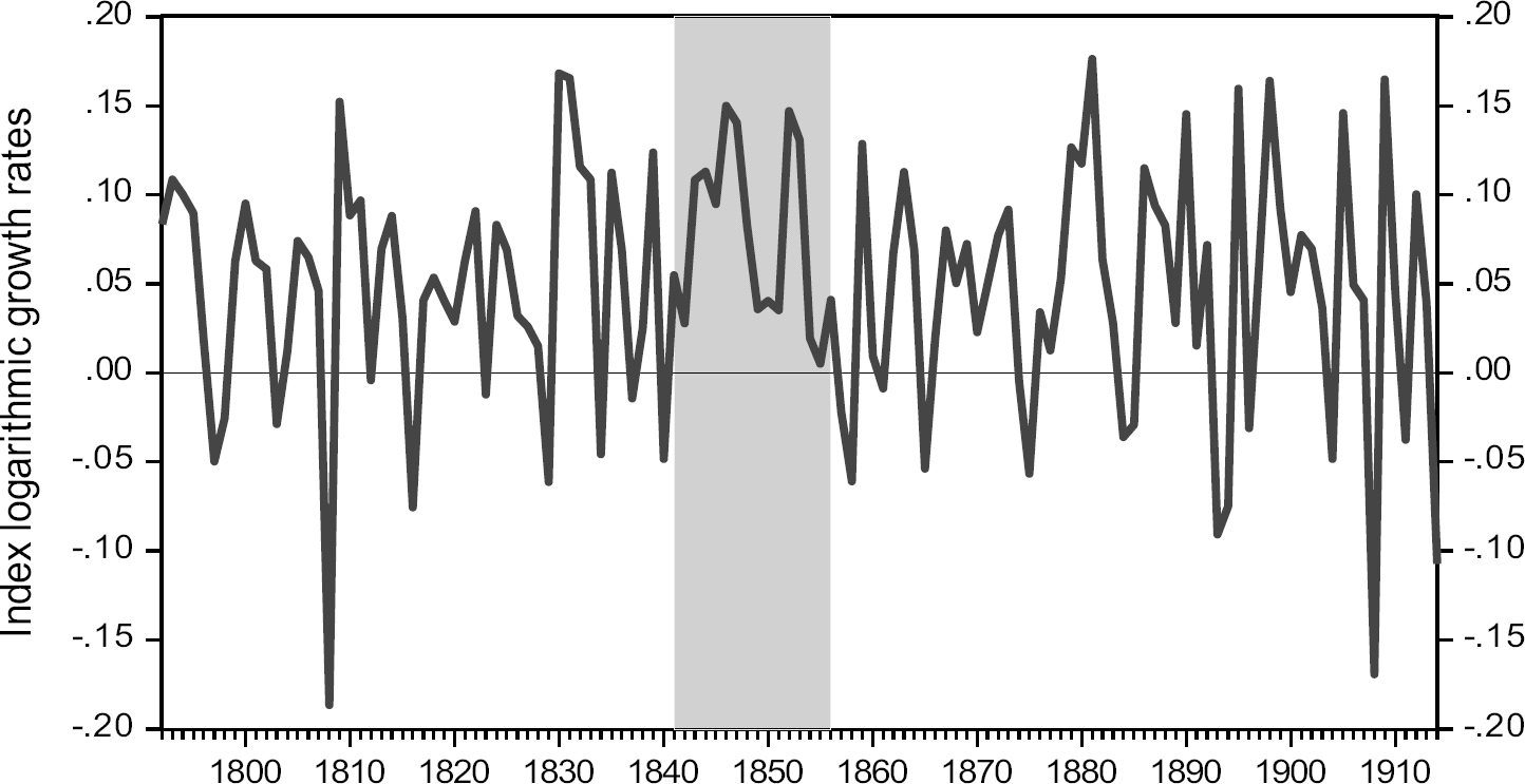
Figure 1 GROWTH RATES IN ANNUAL DAVIS IP INDEX, 1792–1914
Table 1 SUMMARY STATISTICS FOR U.S. INDUSTRIAL PRODUCTION GROWTH, 1792–1914
∗ = Significant at the 10 percent level.
∗∗ = Significant at the 5 percent level.
∗∗∗ = Significant at the 1 percent level.
Sources: Davis (Reference Davis2004); authors' calculations.
During the antebellum period, the differences in average growth rates between the Great Moderation and other years are statistically significant (p=0.04), compared to insignificant differentials between the antebellum and post-bellum periods (see bottom of Table 1). One would expect average IP growth to be higher during the First Great Moderation since there were no absolute annual declines in industrial production between 1841 and 1856. The high rate of growth in industrial production was accompanied by low volatility. The standard deviation of IP growth was 5 percent between 1841 and 1856. For the antebellum period before the start of the First Great Moderation, the standard deviation of industrial production growth averaged 6.7 percent. The standard deviation of IP growth averaged 7.5 percent in the post-bellum period. As is the case with mean growth rates, volatility differences in IP growth between the Great Moderation and the antebellum years between 1792–1840 are statistically significant (p=0.098), compared to insignificant differentials between the antebellum and post-bellum eras (p=0.355). We also employ the coefficient of variation (standard deviation divided by the mean) to control for the fact that the average growth rate in IP was higher during the First Great Moderation. Table 1 shows that the coefficient of variation for industrial production during the First Great Moderation, at 0.65, was notably lower when compared to 1.45 for the antebellum period and 1.63 for the post-bellum period. The basic summary statistics indicate that industrial production growth was higher and IP volatility significantly lower during the First Great Moderation.
We corroborate our annual IP-based results using a monthly series on stock prices, which should afford an even higher-frequency indicator of financial conditions and “panics” sometimes cited in the qualitative characterizations of the contemporary economy. Specifically, we employ William N. Goetzmann, Roger G. Ibbotson, and Liang Peng's (2005, hereafter GIP) pre-CRSP era stock index from 1815–1914 to examine stock returns and stock volatility during the First Great Moderation. The GIP pre-CRSP era NYSE series is among the most comprehensive monthly stock market series for the nineteenth century. While other city-level stock price series exist for the antebellum period (Schwert Reference Schwert1990), we focus on the GIP series since it spans the entire nineteenth century and tends to include more securities than other stock indices, such as Smith and Cole's price index (Smith and Cole Reference Smith and Cole1935).
Table 2 shows that stock returns averaged 0.3 percent per month during the Great Moderation. Average stock returns for the GIP Index were negative in the antebellum period before the Great Moderation, and averaged 0.17 percent per month in the post-bellum period. Stock volatility, as measured by the standard deviation of monthly price returns, averaged 3.5 percent during the First Great Moderation, compared to 3.9 percent and 4 percent in the antebellum and post-bellum periods, respectively. The lower stock-market volatility for the Great Moderation is statistically significant and is more than 20 percent lower than the non-Great Moderation antebellum period and more than 10 percent lower than the post-bellum period. The coefficient of variation for stock returns during the First Great Moderation, 11.44, is approximately one-half that of the coefficient of variation for either the earlier antebellum period (25.78) or post-bellum period (23.35). Overall, we find that stock returns were both higher and significantly less volatile than the rest of the pre-WWI period.
Table 2 SUMMARY STATISTICS FOR EARLY U.S. STOCK RETURNS, 1826–1914
∗ = Significant at the 10 percent level.
∗∗ = Significant at the 5 percent level.
∗∗∗ = Significant at the 1 percent level.
Sources: Goetzmann et al. (Reference Goetzmann, Ibbotson and Peng2001); authors' calculations.
IDENTIFYING BUSINESS CYCLES
Focusing on industrial production rather than broad GDP or even nonagricultural GDP could be a potential limitation of our study if (and only if) IP was not reflective of the broader economy during this era. We argue that this was not the case, for several reasons. As discussed in Davis (Reference Davis2004), IP is appropriate to define the historical evolution of U.S. business cycles, if for no other reason than the fact that America's emergence as an economic power is commonly equated with its industrialization. While more than one-half of national output in the antebellum United States was agricultural, the Davis IP index should be broadly indicative of the nation's economic conditions because the industrial sector has historically derived demand directly from nonindustrial occupations, particularly farmers, merchants, and the construction trades.Footnote 11 The processing of foodstuffs, the demand for agricultural machinery, and the capital equipment required to transport agricultural commodities to market are all intimately tied to farm output and the relative price of agricultural goods, even though agricultural production is often characterized as acyclical. Likewise, the manufacture of lumber products and transportation equipment were acutely sensitive to business conditions in the construction trades, the railroad industry, and inland transportation sectors.
Some of the most severe contractions in the Davis IP index were the result of a significant shock originating in the non-industrial sector. A prime example is the deep recession of 1808, when the Davis IP index contracted nearly 19 percent given the collapse of the shipbuilding and foodstuff industries that were heavily dependent upon the health of the maritime trades and Britain's export market. Indeed, the non-intercourse period following the Embargo of 1807 had a devastating impact on the economy despite temporarily stimulating some infant industries and led to the largest annual decline in the Davis IP index in the pre-Civil War era. Finally, the NBER today includes industrial production (and not GDP) as one of the four primary coincident indicators to identify and date U.S. business cycles. While IP is less comprehensive than GDP, it is both valuable and accurate in identifying turning points today since manufacturing is a highly-cyclical sector, in the same way it was for the antebellum period. This is important considering that the economy's share of output in the industrial sector over the past three decades (roughly 20 percent) was similar to its share between the 1840 and 1860.
COMPARING TWO GREAT MODERATIONS
We examine the robustness of our identification of the First Great Moderation in two related ways. First, we judge how America's Second (modern-day) Great Moderation looks using comparable annual IP fluctuations. Second, we estimate Markov regime-switching models to assess the statistical significance of America's First Great Moderation, and again compare those estimated results to same-frequency IP and stock-price data observed for the Second Great Moderation. We can get a general sense of the magnitudes of the two Great Moderations by creating trailing growth-to-volatility ratios in an annual IP index that spans both. We accomplish this by creating one extended annual IP series from 1790 through 2010 according to the procedures recommended in Davis (Reference Davis2004). Specifically, we ratio-splice the annual Davis IP index to the Miron-Romer IP index in 1916 before ratio-splicing to annual values of the Federal Reserve IP index beginning in 1919. While we stress that we cannot conduct a formal statistical volatility break-point test on this long series given changes in series comparability and reliability over time, the growth-to-volatility ratio in Figure 2 allows us to visually gauge changes over rolling 20-year periods. Clearly, Figure 2 suggests that the combination of high IP growth and lower IP volatility during America's first Great Moderation appears to have been as impressive in scale as America's second (modern-day) Great Moderation when measured against similar annual IP index data from the Federal Reserve.
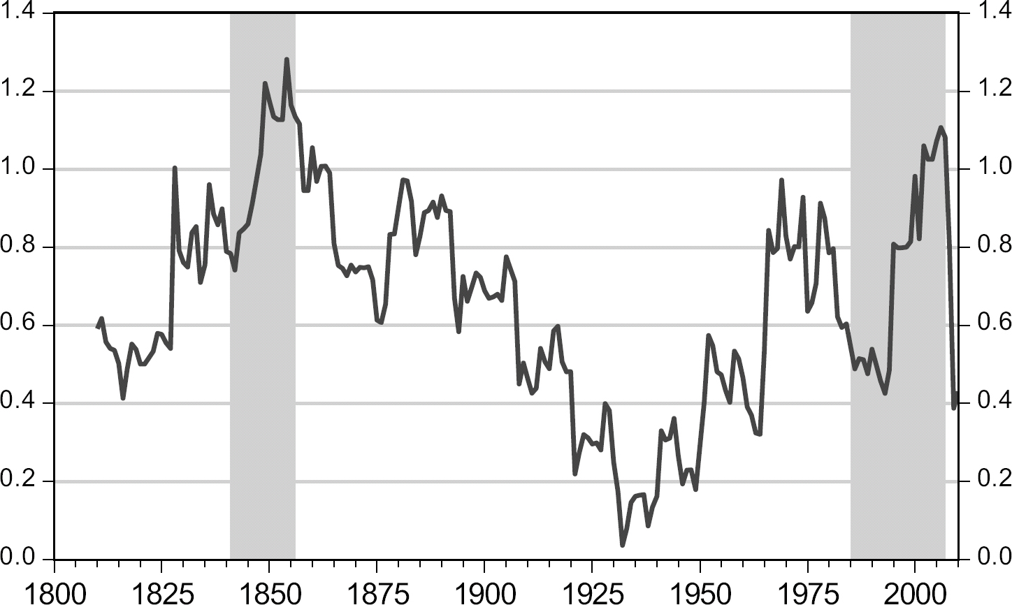
Figure 2 GROWTH-TO-VOLATILITY RATIO IN INDUSTRIAL PRODUCTION, 1810–2010
We can also examine the business-cycle properties in the Second Great Moderation by dating recessions simply by declines in the annual IP index over the 1980–2010 period. As shown in the first column of Table 3, recessions are denoted by parentheses which indicate a decrease in the IP index. The recessions of 1991, 2001, and 2008–2009 clearly show up in the Federal Reserve's annual IP data.
Table 3 COMPARING THE TWO GREAT MODERATIONS USING ANNUAL IP DATA
Notes: Hodrick-Prescott filters used lambda=100.
Sources: Authors' calculations based on data from Davis (Reference Davis2004) and U.S. Federal Reserve.
“Growth recessions” are identified in either of the Great Moderation periods by calculating deviations from the trend in the annual log IP series (i.e., an “IP gap”) of the Davis and Federal Reserve series, respectively. To span most definitions of fluctuations versus trends, we estimate trends two ways: (1) a one-sided, backward-looking Hodrick–Prescott (HP) filter, and (2) a two-sided HP filter that possesses look-ahead bias. We report deviations from trend growth in the columns labeled “1-sided HP filter and “2-sided HP filter” in Table 3. The empirical results show that while America's First Great Moderation did not involve an outright decline in real output, the U.S. economy did experience several so-called “growth recessions” at times when real output increased at a below-trend pace. Important examples during the First Great Moderation include the early 1840s following the Panic of 1839, as well as respites from otherwise strong growth in the late 1840s and the mid-1850s, periods that Thorp misclassified as recessions (Davis Reference Davis2006). For the Second Great Moderation, similar growth recessions persist through roughly half of the 1984–2007 period. Using a one-sided real-time measure of deviation from trend, the U.S. economy did not grow above trend in any year between 2001 and 2010.
We estimate Markov regime-switching models to assess the statistical significance of changes in real economic volatility (high-vol, low-vol) before, during, and after the First Great Moderation using logarithmic growth rates in annual IP growth (1792–1914). We then compare our results to America's Second Great Moderation using similar data and techniques for the post-WWII period. Our primary specification is a univariate autoregressive non-linear Markov-switching model with two regimes. In particular, we assume that annual IP growth, ![]() , depends on two underlying and unobserved states,
, depends on two underlying and unobserved states, ![]() such that:
such that:
At first pass, we allow the means, variances, and autoregressive parameters to all vary between two states. We then also impose a constant-mean restriction based on the equality-of-means tests in Table 1, still allowing the variance and autoregressive parameters to vary between two states.
The Markov-model results for annual IP growth over the entire pre-WWI, 1792–1914 sample are reported in Table 4, Panel A. All estimated parameters are statistically significant at the 10 percent significance level or better, with significant differences in volatility between the high-volatility and low-volatility states. Annual IP volatility in the low-volatility regime was approximately one-fourth that of high-volatility regime (0.27). The average mean growth rates estimated in the Markov-switching models is 4.29 percent per annum.Footnote 12 Table 4 also compares the constant-mean results for the 1792–1914 period (Panel A) with those for annual IP data for the 1950–2010 period (Panel B). While the estimated standard deviation in the low-volatility state is marginally significant (p=0.12) in the later period, the standard deviation of the low-volatility state is almost 1/25th the size of the high-volatility state. The results from the Markov-switching model suggest that business cycle volatility was much less in the low-volatility state relative to the high volatility state, especially during the Second Great Moderation.
Table 4 MARKOV REGIME-SWITCHING MODELS FOR IP GROWTH
∗ = Significant at the 10 percent level.
∗∗ = Significant at the 5 percent level.
∗∗∗ = Significant at the 1 percent level.
Notes: Model specification is an AR(1) switching-variance model with constant mean.
Sources: Authors' calculations and output from Markov-Regime Switching Model.
Panels A and B of Figure 3 show the low-volatility state probabilities from the Markov models for the Davis and Federal Reserve Board industrial production indices.Footnote 13 Panel A of Figure 3 confirms that the First Great Moderation began in the early 1840s and ended in 1857, with the probability of a low-volatility state rising to nearly 90 percent in the late 1840s and early 1850s. The peak during the First Great Moderation is higher than at any other time during the 1792–1914 period. In a similar fashion, the probability of a low volatility state is highest during America's Second Great Moderation. Again, the probability of a low-volatility state peaks during the mid to late 1990s and early 2000s.

Figure 3 LOW-VOLATILITY STATE PROBABILITIES FOR ANNUAL U.S. IP GROWTH RATES
Figure 4 compares the First Great Moderation with the Second Great Moderation by plotting the ratio of the conditional mean to the conditional standard deviation for the growth rate of the two industrial production series. The growth rate of the two IP series shows a spike in the ratio that coincides with a Great Moderation in the pre-WWI era as well as one in the modern era. By this metric the First and Second Great Moderations were very similar in relative magnitudes.Footnote 14

Figure 4 RATIO OF CONDITIONAL MEAN TO CONDITIONAL STANDARD DEVIATION IN ANNUAL IP
SOURCES OF THE FIRST GREAT MODERATION IN INDUSTRIAL PRODUCTION
We hypothesize that a primary factor for the Great Moderation in both manufacturing and in the U.S. stock market was the diffusion of technologies centered in the transportation sector. Such technological diffusion would have generated spillovers in the form of increased investment, larger and more integrated product and labor markets, and increased western migration within the United States. Indeed, the First Great Moderation was characterized by the accelerated adoption of three important transportation and communication technologies: (1) the steam locomotive and railroad, (2) faster clipper and steam ships, and (3) the telegraph.
According to George R. Taylor (Reference Taylor1951), the 1840s and 1850s marked a “transportation revolution” in the antebellum U.S. economy that witnessed strong gains in productivity and high levels of investment. Trend economic growth was high in part due to high rates of both public and private investment in expanding transportation networks for roads, canals, railroads, and global shipping routes. During the 1840s and 1850s, American shipyards built more merchant tonnage than what was built in the previous four decades combined. Indeed, the zenith in merchant tonnage constructed in 1854 and 1855 would not be surpassed until WWI. Before the Civil War, the shipbuilding industry was large, representing more than 5 percent of the total value added in the industrial sector, exceeding the value added of locomotive production (3.6 percent weight in the Davis IP index). A primary factor in the surge in shipbuilding investment was the clipper ship, an extremely fast ship that possessed flatter hulls, sharper bows and could routinely accommodate more than 2,000 tons in cargo. The discovery of gold in California in 1848 led to an immediate jump in the expected rates of return on fast ships that could quickly carry large cargoes to San Francisco and then sail to China (for its valuable tea). The fastest clipper ships built in the 1850s in the shipyards of New York, Boston, Philadelphia and Maine could cost nearly $3.13 million in current 2016 U.S. dollars to construct at the time, but they could sail from the eastern coast to San Francisco via the Cape Horn in as little as 90 days. One round-trip could net a profit for ship owners equal to the entire cost of construction (Howe and Matthews 1986).Footnote 15
The period from the late-1840s through the mid-1850s is generally known as the “Clipper Ship Era.” The production of clipper ships increased from an index value of 58 in 1841 to a value of more than 158 in 1856. The period 1850 until 1856 represented the high point, an index value of 266 in 1854, for the clipper ship which benefitted from the gold rush in California and the China trade. Clipper ship production started to wane in 1857 as the clipper ship gradually gave way to steam powered ships that could carry heavier loads across the Atlantic and Pacific Oceans. The boom in clipper-ship construction had a significant economic impact on the U.S. lumber industry, with many coastal timber fields being exhausted during the 1850s given the demand for lumber products to construct the large wooden ships. Steamship trade also experienced a take-off during the First Great Moderation. The number of steamships involved in the Atlantic trade increased from 5,631 tons in 1847 to 97,296 tons in 1860 (Taylor Reference Taylor1951, p. 116).
Steam was also used to power rolling stock during the antebellum period. It took a few decades of innovation and capital investment before the railroad had a large impact on the antebellum economy. Rail mileage accelerated through the 1830s and 1840s, reaching 3,328 miles in 1840 and 8,879 by 1850. By 1850, railroad mileage had outpaced canals in 25 states. Both experienced an increase in tonnage in the West, but for water routes this was largely the result of massive Western migration, which increased demand across the board. This technological-diffusion process accelerated with the construction of almost 22,000 miles of track built in the 1850s. By the eve of the Civil War, railroads had replaced canals as the predominant means of transportation.Footnote 16
To explore whether transportation played a critical role in America's First Great Moderation, we created special sub-indices of the Davis IP series. We decompose the Davis IP index into two broad, mutually-exclusive sub-indices—an investment goods IP index and a consumption goods IP index. The investment goods index consists mostly of durable goods, including metal-producing sectors, transportation machinery, other small machinery categories, and the lumber industry. The consumption goods index consists of the food, textiles, printing, chemical/fuels, and leather-producing sectors.Footnote 17 In 1850, the consumption goods industry accounted for approximately 60 percent of the total value added in the manufacturing and mining sectors, while manufacture of investment goods yielded the remaining 40 percent of industrial production.
We construct even finer-level IP indices from both the investment and consumption goods IP indices. For consumption goods, we create two IP indices—an IP food products index (accounting for 10.9 percent of the value-added in the industrial sector in 1850) and an IP textiles index (21.8 percent), which is primarily comprised of the cotton consumed by domestic textile mills. During this period, the textile sector was the largest industry on both a gross and value-added basis. For investment goods, we create an IP metals index (accounting for 12.9 percent of the value added in 1850) and an IP transportation-intensive index (22.7 percent) comprised of locomotive production, shipbuilding, and the primary input by far to ship construction at that time, lumber. Finally, we created an IP index excluding transportation-intensive sectors that accounts for the remaining series in the Davis IP index, accounting for 77.3 percent of that index on a value-added basis. We then calculate growth rates, standard deviations, and coefficients of variation for all of these IP series as we did for the aggregate index. The summary statistics are reported in Table 5. Several important features emerge. Both consumption and investment goods had higher rates of average growth during the Great Moderation than either before or after, although the boom in investment goods during the 1841–1856 period is much stronger, with growth in the transportation IP index averaging 10 percent per annum versus only 3 percent per annum in the 1792–1840 period. The U-shaped pattern in volatility for the Davis IP index—lower volatility during the Great Moderation versus the periods before and after—is observed for investment goods, but not for consumption goods. The standard deviation in transportation-related production declines by one-third between the antebellum (0.179) and Great Moderation period (0.115) before nearly doubling in the post-bellum period (0.207). The decline in volatility in metals production is less pronounced and more monotonic throughout the 1828–1914 period.Footnote 18
Table 5 SUMMARY STATISTICS FOR IP COMPONENTS
Notes: All data expressed in logarithmic growth rates (except for tariffs) and are available back through 1792 except for IP metals (1828 with introduction of pig iron) and the immigration rate (1821). The IP index for consumption goods includes the Davis (Reference Davis2004, Table II, p. 1188) sector series for food products, textiles and apparel items, leather, printing and publishing, and chemical and fuel products. The IP investment goods index constitutes the remainder of the Davis IP index and includes metals, lumber, transportation equipment, and other small machinery categories (musical instruments, scientific equipment, and ordnance).
Sources: Authors' calculations based on Davis (Reference Davis2002, Reference Davis2004), Carter et al. Reference Carter, Gartner and Haines2006, Parts C and D, and NBER Macrohistory Database.
The combination of higher growth and even lower volatility for investment goods leads to a pronounced U-shaped pattern in the coefficient of variation for the investment goods IP index. The coefficient of variation for investment goods is 0.81 for the Great Moderation, or 80 percent lower than for the earlier antebellum period (4.15) and nearly one-third lower than the post-bellum period (2.65). This U-shaped pattern in the coefficient of variation is even more striking for the transportation-goods sector, with a ratio of 1.15 during the Great Moderation, a fraction of that observed either before (6.02) or after the Civil War (14.08). Overall, the summary statistics in the top half of Table 5 would suggest that transportation-related investment contributed to the emergence of America's First Great Moderation.
We test our hypothesis that transportation-related investment was the primary source of the recession-free period from 1841–1856. Again, we estimate the Markov regime-switching model on the IP indices that exclude textiles, transportation, and investment/consumption goods, respectively. In doing so, we can assess whether the exclusion of a primary sector (i.e., transportation or textiles) significantly weakens the probability that the Great Moderation would have occurred. Figure 5 displays the probability that a series was in a low-volatility state for each year based on the Markov regime-switching model.Footnote 19 Most notably, the Great Moderation is much weaker when one excludes transportation-goods investment, with only the 1843–1849 period possessing probabilities above 50 percent. The implication is that without transportation investment, the U.S. economy would have only experienced a moderate expansion that ended before 1850 and would not have experienced the high growth of the 1850s. Second, the Great Moderation in investment goods is clearly evident in Figure 5; before 1841 the investment goods sector was rarely estimated to have been in a low-volatility state compared to the broader Davis IP index. Third, the results for the IP index excluding textiles in Figure 5 suggest that the Great Moderation may have persisted even longer had there not been more significant and negative impacts from the volatility in cotton textile production in the late 1850s.

Figure 5 PROBABILITIES OF LOW VOLATILITY STATES FOR IP WITH AND WITHOUT KEY SECTORS
The Markov-based results strongly suggest that the boom in transportation investment was a key contributor to America's First Great Moderation. To better infer whether such investment spilled over to or led other economic activity, we run bivariate Granger-causality tests between each of the four key sectors (all investment goods, transportation, metals, as well as textiles) on all other IP. We run these tests for the entire 1792–1914 sample, as well as for three sub-samples.Footnote 20 First, we find transportation IP led all other IP during the Great Moderation period at the 0.01 significance level, while all other IP did not lead fluctuations in transportation production. Transportation IP statistically led growth in consumption-goods output, too, during the Great Moderation (p=0.03). Second, the results are exactly the opposite for textiles and metals, where all other IP led textile and metal IP during the Great Moderation at the 0.02 and 0.05 significance levels, respectively. Third, growth in transportation-related IP did not lead all other IP growth during the postbellum period; rather, the lead relationship ran in the opposite direction. We also tested whether the cotton crop, tariffs, or British IP lead changes in overall U.S. industrial production during the Great Moderation. The three variables did not Granger-cause the growth rate in the Davis industrial production series. Overall, the 1841–1856 period was unique in how the boom in transportation investment contributed to a period of higher growth and lower volatility.
CONCLUSION
The Great Moderation that commenced around 1984 is regarded by many economists as one of the longest periods of economic growth and low business cycle volatility in American history. In this article, we identify another, much earlier period of high economic growth and low economic and financial market volatility. America's First Great Moderation—a recession-free, 16-year period from 1841 until 1856—represents the longest economic expansion in U.S. history. The growth rate of industrial production was exceedingly high; annual growth in industrial production averaged nearly 8 percent per annum, the fastest pace of economic growth in the nineteenth century.
We believe that America's antebellum “transportation revolution” was a significant driver of the First Great Moderation. We show that America's First Great Moderation was largely driven by transportation-goods investment, which we attribute to the wider adoption of new technologies for railroad and shipbuilding industries.
Markov regime-switching models reveal that the low-volatility derived for the First Great Moderation was of similar relative magnitude and statistical significance to those estimated for the Second Great Moderation using comparable economic and stock-market data. This may make sense given several similarities between the 1841–1856 and 1984–2006 periods. Both moderations experienced a change in the structure of the economy. The First Great Moderation witnessed the widespread adoption of new technologies—clipper and steam ships, railroads, and the telegraph—that helped contribute to significantly larger markets for goods, labor and exports. The modern Great Moderation saw structural change in terms of the movement of production from goods to services, the IT revolution that led to better inventory management and financial innovations that allowed households and firms to better smooth consumption and investment. In addition, the first and second moderations may have been characterized by improved economic policymaking. Many states during the first Great Moderation wrote new constitutions that redefined the rules of the game for business and the government. As for the modern period, many scholars, including Ben Bernanke (Reference Bernanke2004), have argued that good monetary policy was an important factor in the Great Moderation from 1984–2007. Finally, both periods seem to have benefitted from good luck. While we do not observe significant changes in weather shocks or commodity prices during this period, it is likely that the first Great Moderation benefitted from the discovery of gold in California. It also occurred during the era of Pax Britannica—a period of global peace (Brown et al. 2005) even though the United States fought in the Mexican-American War (1846–48). The second Great Moderation, on the other hand, appears to have been a period of generally low and stable oil prices coupled with few negative productivity shocks, at least up until 2007.
In summary, our analysis suggests that the First Great Moderation was characterized by high economic growth rates and low business cycle volatility. Like the modern-day Great Moderation, the end of America's First Great Moderation was abrupt, pronounced, and notable for its magnitude following years of relative stability. Unlike the modern-day Great Moderation, however, America's First Great Moderation occurred despite a low level of government spending, the absence of a central bank, and no marked improvement in price stability.
Ultimately, the findings in our article may help alter not only how economic textbooks characterize the nineteenth-century economy, but today's business cycle as well.


