


I. INTRODUCTION
Hyperspectral images (HSIs) contain hundreds of contiguous spectral bands ranging from visible to infrared bands, which can provide rich spectral information [Reference Plaza1]. Compared with multispectral images with only a few spectral bands, they offer an advantage in terms of classification and detection [Reference Xu, Du, Li, Chen and Younan2]. Due to the rich spectral bands, HSIs have a variety of applications including environmental pollution control, agriculture precision farming, mineral exploration, etc [Reference Lillesand and Kiefer3–Reference Mei, Ji, Geng, Zhang, Li and Du6]. Accurate classification is very important to those applications. The key for accurate classification is to learn an accurate similarity metric between samples. The traditional pixel-wise algorithms assume the samples from the same class have similar spectral characteristics and simply compare the similarity between pixels. However, for a complicate HSI scene, different materials might have a similar spectral signature, and pixels from the same class usually have various spectral signature. Thus, it is quite difficult to distinguish them by simply comparing the spectral distance. Additionally, the limited number of training samples and the high dimensionality, also known as the Hughes Phenomenon, prohibit the performance of HSI classification [Reference Yang, Du and Chen7].
To overcome the above-mentioned problems, kernel-based approaches have been applied for HSI classification and shown excellent performance [Reference Liu, Fowler and Zhao8–Reference Kuo, Ho, Li, Hung and Taur10]. Kernel methods project the original samples into a high-dimensional space, where the samples are more separable. The commonly used kernels include Gaussian radial basis function (RBF), Polynomial, and linear kernels [Reference Melgani and Bruzzone11]. In [Reference Camps-Valls and Bruzzone12], kernel-based Support Vector Machine (SVM) is proposed for HSI classification. A region-kernel-based SVM [Reference Peng, Zhou and Chen13], which measures the region-to-region similarity, is able to capture the spatial–spectral similarity and has shown improved performance. Other variants such as generalized composite kernel [Reference Li, Marpu, Plaza, Bioucas-Dias and Benediktsson14] and sample-cluster composite kernels [Reference Gomez-Chova, Camps-Valls, Bruzzone and Calpe-Maravilla15] are also introduced for spectral–spatial HSI classification. In [Reference Sun, Liu, Xu, Tian and Li16], a band-weighted SVM, which generates a band weight vector to regularize the original SVM, is presented for HSI classification. Kernel collaborative representation with Tikhonov regularization is presented for HSI classification in [Reference Li, Du and Xiong17, Reference Ma, Mei, Wan, Hou, Wang and Feng18].
Although kernel methods have achieved excellent performance for HSI classification, the kernels are constructed using the distance between the training samples only while ignoring the available label information. The label information among the training samples can be used to help refine the original kernel. In [Reference Kwok and Tsang19–Reference Pan, Chen, Xu and Chen21], the ideal kernel method is presented which incorporated the label information into the original kernel and has shown better performance compared to using the original kernel only. An ideal regularized composite kernel (IRCK) framework is applied for HSI classification in [Reference Peng, Chen, Zhou and Li22], which combines spatial information, spectral information, and label information simultaneously. Multiple Kernel Learning (MKL) [Reference Mehmet and Alpayd23], which combines multiple kernels to improve the performance, has been applied for HSI. A composite kernel approach, which balances the spatial and spectral information, is presented in [Reference Camps-Valls, Gomez-Chova, Muñoz-Marí, Vila-Francés and Calpe-Maravilla24], and four types of different composite kernels are proposed including summation kernel, weighted summation kernel, stacked kernel, and cross-information kernel. In [Reference Wang, Gu and Tuia25], a two-step discriminative MKL (DMKL), which can increase the between-class scatter while decrease the within-class scatter in the reproduce kernel Hilbert space, is presented for HSI classification.
The abovementioned IRCK method incorporates the spatial information in terms of the spatial mean pixel of the neighborhood; however, it does not consider other different types of spatial information, which may provide complementary discriminative information. Different types of spatial features have been widely investigated for HSI classification. For instance, in [Reference Li and Du26], a Gabor-filtering-based nearest regularized subspace is presented for HSI classification. In [Reference Li, Chen, Su and Du27], local binary pattern is applied to extract local image features such as edges, corners, and spots, and then extreme learning machine is applied to achieve excellent performance for HSI classification. In [Reference Dalla Mura, Atli Benediktsson, Waske and Bruzzone28], extended multi-attribute profiles feature (EMAP) is presented for the analysis of hyperspectral imagery, which can efficiently extract the spatial information for classification purposes.
Furthermore, for a complicated HSI scene, one type of feature may not guarantee good performance, especially when the number of training samples is small. Different types of features can be used to provide more discriminative information, and multiple feature learning can be a good solution to solve the above limitation. For instance, a multiple feature learning framework, which integrates both linear and non-linear features, is introduced for HSI classification [Reference Li29]. In [Reference Li, Zhang and Zhang30], a non-linear joint collaborative representation model with multiple feature learning is presented to solve the small sample set problem in HSI. An efficient patch alignment framework, which combines multiple features, is proposed in [Reference Zhang, Zhang, Tao and Huang31].
Inspired by the idea of multiple feature learning, in this paper, we propose to combine different types of features for the IR kernel. Four types of features including spectral feature, Gabor feature, EMAP feature, and LBP feature are investigated due to their potential for HSI classifications. Moreover, a majority voting-based ensemble approach is adopted to make more robust classifications. The rest of the paper is organized as follows. The related work on regularized kernel is introduced in Section II. Section III shows the proposed framework. In Section IV, the experimental results and analysis are provided. Finally, Section V draws the conclusion.
II. REGULARIZED KERNEL
A) Standard kernel
Suppose we have a set of HSI training samples $\varsigma = \{ ({\boldsymbol{x}_1},{y_1}),({\boldsymbol{x}_2},{y_2}), ..., ({\boldsymbol{x}_N},{y_N})\}$ with ${\boldsymbol{x}_i} \in {\Re ^d}$
 , where d denotes the dimensionality of a sample. The kernel measures the similarity between two samples. The most commonly used kernels are linear kernel, polynomial kernel, and RFB kernel. We choose the RBF kernel in our experiment due to its wide application for HSI classification, and the RBF kernel is calculated as

where $\delta$ is the band width of the RBF kernel.
B) Ideal kernel
The ideal kernel is defined as [Reference Pan, Lai and Shen20]

The ideal kernel is inspired by the idea that if two samples should be considered as “similar” if and only they belong to the same class. The ideal kernel has included the label information.
C) Ideal regularized kernel
The similarity measurement between samples in the standard kernel does not consider the labeled information, and a more desirable kernel can be learned by incorporating the labeled information. In [Reference Pan, Chen, Xu and Chen21], an ideal regularization (IR) learning framework is proposed, which can efficiently incorporate the label information into the standard kernel. The following equation learns a more desirable matrix K given the initial kernel ${\boldsymbol{K}_0}$ [Reference Pan, Chen, Xu and Chen21]

where D represents the von Neumann divergence between $\boldsymbol{K}$ and ${\boldsymbol{K}_0}$
 , ${\Omega}$
 is a regularization term, and $\gamma$
 is the regularization parameter. $\boldsymbol{K}\,{\succeq}\,0$
 indicates that $\boldsymbol{K}$
 is a symmetric positive semidefinite matrix. The von Neumann divergence is expressed as

where tr(•) represents the trace of a matrix and ${\Omega}$ (K) is defined as ${\Omega} (\boldsymbol{K}) = - {\rm tr}(\boldsymbol{KT})$
 . The functionality of this term is to incorporate the label information into the standard kernel. Therefore, the final objective function is:

Taking the derivative regarding K and setting the equation to zero, the following equation for K is derived as

where * represents the element-wise dot product between two matrices. Using the Taylor expansion of equation (6), it can be also expressed as:

The above equation indicates that the IR kernel $\boldsymbol{K}$ can be considered as a linear combination of the standard kernel and the ideal kernels.
The out-of-sample extension is investigated for samples that are not encountered before. Denote $\boldsymbol{S} = {{{\rm K}}_0}^{ - 1}(\boldsymbol{K} + {\boldsymbol{K}_0}){\boldsymbol{K}_0}^{ - 1}$ , then the kernel between the two new points $\boldsymbol{s}$
 and $\boldsymbol{t}$
 can be calculated as

D) Majority voting-based ensemble approach
We propose to use a majority voting-based ensemble approach to combine the output of SVM using the IR kernel with different types of features. Suppose we are using m features and ${f_i}(\boldsymbol{x})$ represents the output using the i-th feature, the final output is calculated as

III. PROPOSED FRAMEWORK
In this paper, a majority voting-based multi-feature IR kernel method which can efficiently deal with the small training sample problem is proposed. Figure 1 shows the proposed framework. First, principal component analysis [Reference Rodarmel and Shan32] is conducted on the original dataset to extract the principal components of the original dataset. Different types of features including EMAP features, Gabor features, and LBP features are then extracted from the principle components. Classification is conducted on each type of feature with the IR kernel-based SVM. Finally, a majority voting-based ensemble approach is adopted to combine the results of the classification output.
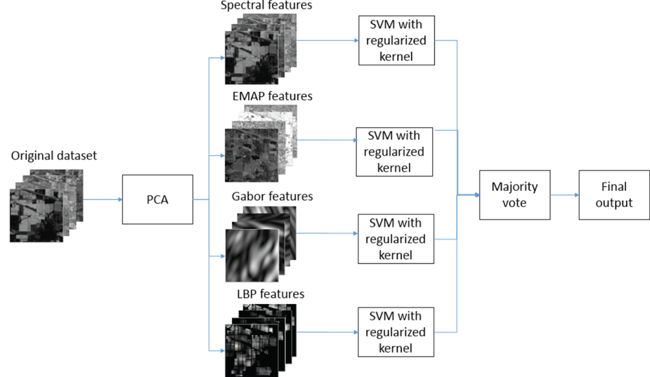
Fig. 1. Proposed framework.
IV. EXPERIMENTAL RESULTS
A) Experimental dataset
Three popular HSI datasets are used in our experiments.
(1) Indian Pines: This dataset is collected by the Airborne Visible and Infrared Imaging Spectrometer (AVIRIS) sensor over the Indian Pines site in June 1992. The spatial size is 145 × 145 with the spatial resolution of 20 m/ pixel. The 200 spectral bands are ranging from 400 to 2500 nm. After bad bands removal, 200 spectral bands remain. There are a total of 16 classes in the scene. The false color infrared of bands 50, 27, and 17 is shown in Fig. 2(a), and the groundtruth is shown in Fig. 2(b).
(2) University of Pavia: The second dataset is acquired by the Reflective Optics System Imaging Spectrometer (ROSIS) sensor, and the scene covers the University of Pavia with 115 spectral bands ranging from 0.43 to 0.86 µm. The spatial size is 610 × 340 with the spatial resolution of 1.3 m/pixel including nine classes. After removing the noisy band, 103 bands remain. Figures 3(a) and 3(b) show the color infrared composite of bands 60, 30, 2 and the groundtruth, respectively.
(3) Salinas: The third dataset is collected by the AVISIS sensor over Salinas Valley, California. The spatial size is 512 × 217 with the spatial resolution of 3.7 m/pixel. After removing the 20 water absorption bands, 200 bands remain. The color infrared composite of bands 47, 27, 13 and the groundtruth is shown in Fig. 4(a), and the groundtruth of this dataset is shown in Fig. 4(b). There are a total of 16 classes.

Fig. 2. Indian pines dataset. (a) Color-infrared-composite of bands 50, 27, and 17. (b) Groundtruth.

Fig. 3. University of Pavia dataset. (a) Color-infrared-composite of bands 60, 30, and 2. (b) Groundtruth.
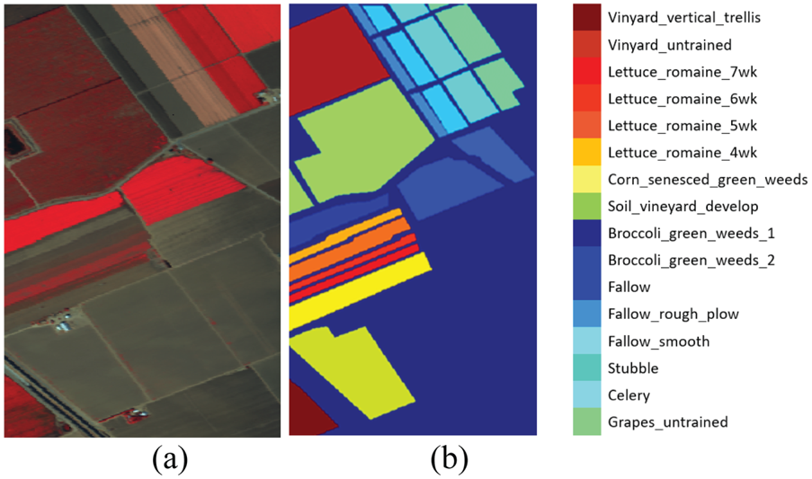
Fig. 4. Salinas dataset. (a) Color-infrared-composite of bands 47, 27, and 13. (b) Groundtruth.
B) Experimental setup
The number of training samples per class is denoted as N. In the experiment, N is chosen to be $\{3, 5, 7,\ldots,13\}$ , and for those classes less than N samples, half of the total samples are chosen for training. The rest of the labeled samples are chosen as the testing set. Gaussian kernel is investigated, and the LIBSVM [Reference Chang and Lin33] is used to implement SVM. The number of PCs for the Gabor features, EMAP features, and LBP features are set to 10, 4, and 4, respectively [Reference Li and Du26–Reference Dalla Mura, Atli Benediktsson, Waske and Bruzzone28]. The EMAP features are generated according to [Reference Dalla Mura, Atli Benediktsson, Waske and Bruzzone28], and the parameters for LBP are set according to [Reference Li, Chen, Su and Du27]. Each experiment is repeated 50 times to avoid bias.
C) Results
Tables 1–3 list the overall accuracies (OAs), average accuracies (AAs) and the κ coefficient of Indian Pines, University of Pavia, and Salinas, respectively, for different types of features using the standard and the regularized kernel; furthermore, a majority voting-based ensemble approach is presented with the standard and regularized kernel to better utilize the discriminative information.
Table 1. Classification accuracies for different features and ensemble approach on Indian Pines.

Table 2. Classification accuracies for different features and ensemble approach on the University of Pavia.

Table 3. Classification accuracies for different features and ensemble approach on Salinas.
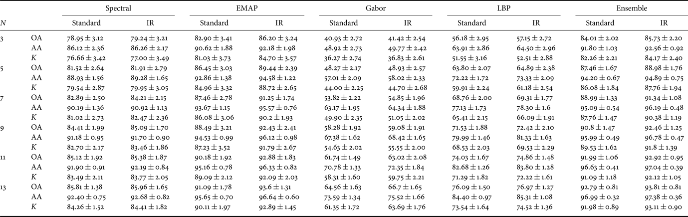
Several observations can be drawn from Table 1. First, the regularized versions consistently outperform the standard kernels using all the four features. Specifically, for the EMAP feature, the regularized kernel can approximately improve the OAs of standard kernel around 5% when the number of training samples is small. For the spectral, Gabor, and LBP, the IR kernels can outperform the standard kernel, indicating the advantage of incorporating the label information into the kernel metric. Second, the majority voting-based ensemble approach can achieve higher OAs compared using a single feature for both the standard and IR kernels. The explanation is that by combining multiple features, complementary discrimination information brought by multiple features is used. Thus, better performance can be achieved. Additionally, the classification performance is improved with the increased number of training samples.
From the results for the University of Pavia, it can be observed that the IR kernel versions can significantly outperform the standard kernel on both the EMAP and Gabor features. For instance, the OAs increase approximately by 3 and 5% on EMAP and Gabor feature, respectively, for the University of Pavia dataset. The IR kernel also has better performance for the spectral feature and LBP feature. Moreover, the ensemble approach using the IR kernel has the best performance, indicating the advantage of combining complimentary discriminative information. It can be observed that the ensemble approach has a smaller variance compared with using a specific feature alone. This is expected because by combining different types of features, a more robust result can be achieved.
For the results on Salinas as shown in Table 3, several conclusions can be drawn. First, it can be concluded that IR can provide better performance compared with the standard kernel for all types of features. For this dataset, ensemble approaches have slightly better performance compared with using the EMAP feature alone. Gabor feature does not have a good performance on this dataset, including the Gabor feature for this dataset can affect the accuracy. We also notice that the regularized kernel has poor performance if the standard kernel has poor performance. In addition, with only seven and 11 training samples per class for Indian Pines, University of Pavia, and Salinas, the OA can be above 90%. The explanation maybe that when the number of training samples is limited, the similarity measurement between samples is not reliable, and thus, the label similarity between different classes can learn a desirable kernel metric, which is essential for good classification performance. Another conclusion is that the ensemble approach provides good performance with a limited number of training samples.
Figure 5 compares the OAs of IRCK, DMKL, and our proposed method using 15 samples per class. It can be concluded that the proposed method has superior performance over IRCK on three different datasets. More specifically, the proposed method has around 6.1, 4.7, and 1.4% higher OA than IRCK for Indian Pines, University of Pavia, and Salinas, respectively. Compared with DMKL, the proposed method has around 7 and 4% higher OA than DMKL on Indian Pines and the University of Pavia, respectively. On the Salinas dataset, the proposed method slightly degrades from DMKL. In Fig. 6, the classification maps of Indian Pines are shown for four different types of features. The proposed method has around 0.6, 4, and 1.5% higher OA for Indian Pines, University of Pavia, and Salinas, respectively. The observation is that few misclassified samples exist in the classification map of the ensemble approaches. This is expected since different features can provide discriminative information, which can lead to better performance.
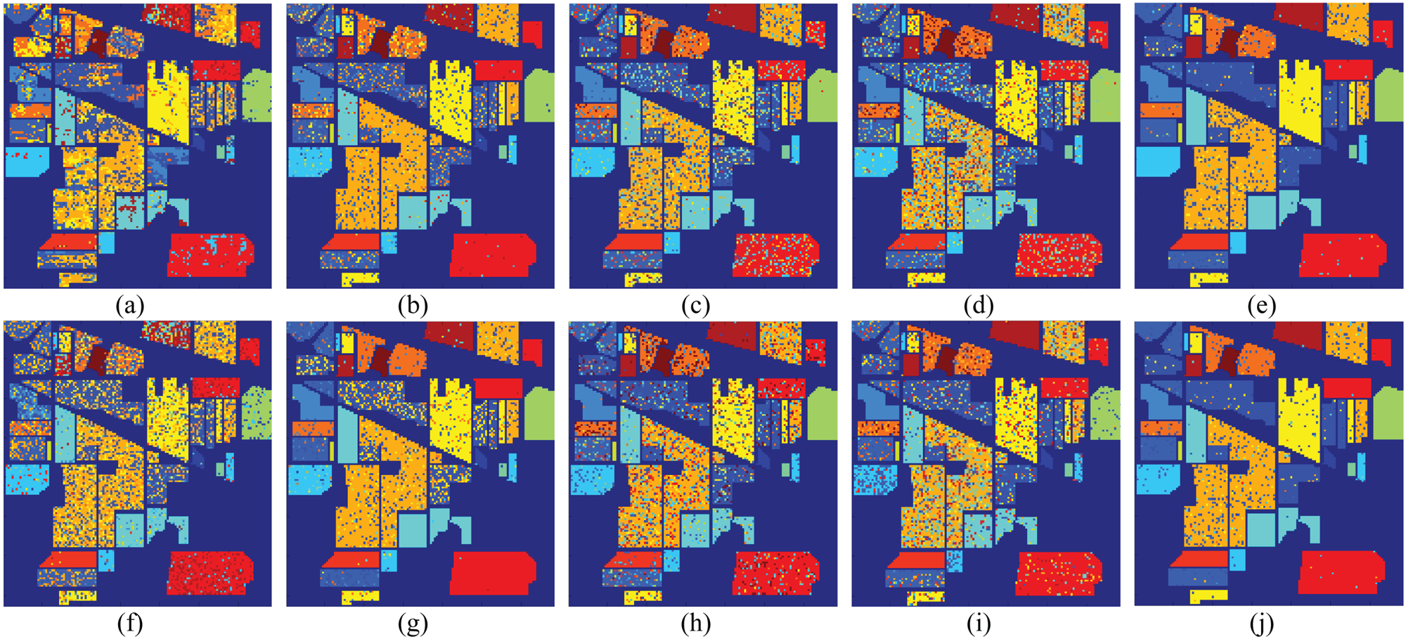
Fig. 5. Overall accuracies of IRCK, DMKL, and the proposed method for three datasets.
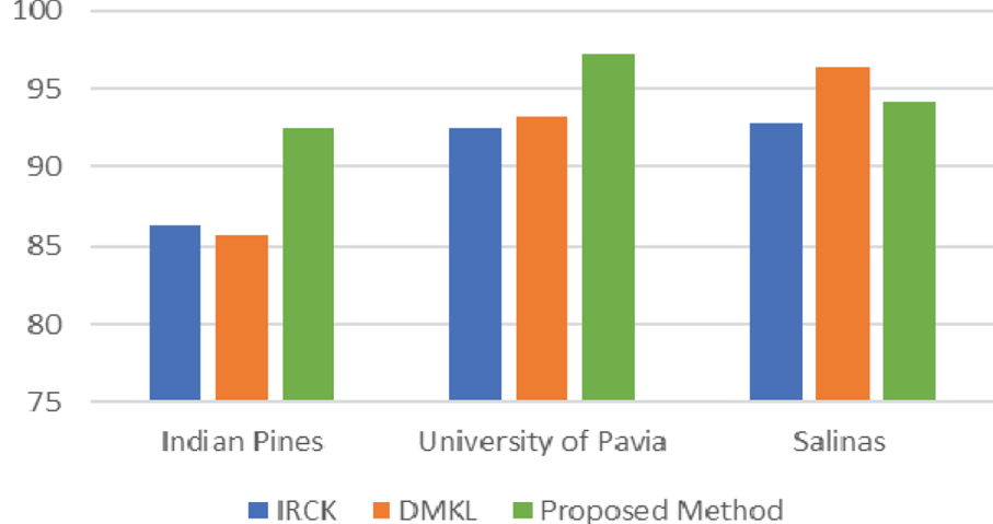
Fig. 6. Classification maps for Indian Pines. The first and second rows correspond to Standard and IR kernels. (a) Spectral-Sta(OA = 63.31%). (b) EMAP-Sta(OA = 83.9%). (c) Gabor-Sta(OA = 77.8%). (d) LBP-Sta (OA = 73.2%). (e) Ensemble-Sta(OA = 92.4%). (f) Spectral-IR(OA = 64.4%). (g) EMAP-IR(OA = 86.4%). (h) Gabor-IR(OA = 78.1%). (i)LBP-IR (OA = 76.8%). (j) Ensemble-IR(OA = 93.8).
D) Parameters analysis
The parameters in this paper are analyzed in this section. For the SVM, we will first analyze the RBF kernel σ and the regularization term C first. For σ, it is chosen from the range {2−4, 2−3, …, 24}. C is chosen in the range {1, 10, 100, 105}. Figures 7(a)–7(c) show the OA with different σ and C for EMAP features on Indian Pines, University of Pavia, and Salinas, respectively, using 13 training samples per class. A holdout validation sample set is used for testing. It can be concluded from Fig. 7 that C does not affect the OA much especially when it is larger than 100, and any number above 100 will guarantee good performance. For σ, a relatively small number will generate good classification performance. In order to analyze the effect of the $\gamma$ parameter in IR, in the following experiment, C is set as 1000, and σ is chosen as 2−1 for the EMAP features of different datasets to ensure good performance.
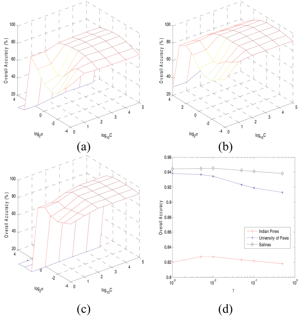
Fig. 7. Parameters tuning using EMAP feature. (a) σ and C for Indian Pines. (b) σ and C for the University of Pavia. (c) σ and C for Salinas. (d) $\gamma$ for all datasets.
The parameter $\gamma$ plays an important role in the classification performance. We investigate the effect of $\gamma$
 on the EMAP feature for Indian Pines, University of Pavia, and Salinas, respectively. Figure 7(d) shows the OAs of the three datasets with respect to different $\gamma$
 in the range {1e−3, 5e−3, …, 5e−1}. It can be seen that the OA stays stable when $\gamma$
 is very small, and when $\gamma$
 increases, the OAs of all three datasets will decrease. This may be due to the reason that the label information is dominant in the generated kernel while ignoring the spectral similarity between the training samples. In our experiment, we set C as 1000, σ as 2−1, and $\gamma$
 as 5e−3 for the EMAP features for three datasets. For other types of features, a similar parameter tuning process is adopted.
V. CONCLUSIONS
In this paper, a novel multiple feature-based IR kernel is presented for HSI classification. The proposed framework incorporates the label information in conjunction with the complementary discriminative information with multiple features. Experimental results show our proposed approach can achieve superior classification performance.
ACKNOWLEDGEMENT
The authors would like to thank Prof. D. Landgrebe for providing the Indian Pines data set, Prof. P. Gamba for providing the University of Pavia data set, and Dr. J. Anthony Gualtieri for providing Salinas data set.
FINANCIAL SUPPORT
This work was supported by the National Natural Science Foundation of China under Grant Nos. 61871177 and 11771130.
Yan Xu received his Ph.D. degree in 2019 from the Department of Electrical and Computer Engineering, Mississippi State University, USA.
Jiangtao Peng received the B.S. and M.S. degrees from Hubei University, Wuhan, China, in 2005 and 2008, and his Ph.D. degree from the Institute of Automation, Chinese Academy of Sciences, China, in 2011. He is currently a Professor in the Faculty of Mathematics and Statistics, Hubei University, China. His research interests include machine learning and hyperspectral image processing.
Qian Du received the Ph.D. degree in electrical engineering from the University of Maryland – Baltimore County, Baltimore, MD, USA, in 2000. She is currently a Bobby Shackouls Professor with the Department of Electrical and Computer Engineering, Mississippi State University, Starkville, MS, USA. Her research interests include hyperspectral remote-sensing image analysis and applications, pattern classification, data compression, and neural networks. Dr. Du is a fellow of SPIE and IEEE. Since 2016, she has been the Editor-in-Chief of the IEEE JSTARS.


 Open access