


1. Introduction
Farms aspire to make the most efficient use of their resources, yet studies indicate that sizable inefficiencies often prevail in agricultural enterprises. Across a broad set of producers and regions, economic efficiency (EE) and technical efficiency (TE) measures in the United States have ranged approximately between 60% and 90% (Aly et al., Reference Aly, Belbase, Grabowski and Kraft1987; Byrnes et al., Reference Byrnes, Fare, Grosskopf and Kraft1987; Chavas and Aliber, Reference Chavas and Aliber1993; Featherstone, Langemeier, and Ismet, Reference Featherstone, Langemeier and Ismet1997; Hall and LeVeen, Reference Hall and LeVeen1978; Mayen, Balagtas, and Alexander, Reference Mayen, Balagtas and Alexander2010; Mugera and Langemeir, Reference Mugera and Langemeier2011; Olson and Vu, Reference Olson and Vu2009; Paul et al., Reference Paul, Nehring, Banker and Somwaru2004; Rowland et al., Reference Rowland, Langemeier, Schurle and Featherstone1998). Removing those levels of efficiency through improved farm management practices would generate savings in input use and production costs by as much as 40%. Identifying inefficiency is thus an important first step in assisting producers to move toward optimal farming outcomes, higher profits, and more socially desirable outcomes. Measuring efficiency is also useful for policy analysts and stakeholders because it can distinguish efficient managers, those making best decisions and utilizing their resource optimally, from less efficient ones. The literature on production efficiency began a few decades ago, seeking to explain how and why certain firms perform better than others (Farrell, Reference Farrell1957; Koopmans, Reference Koopmans1951). Efficiency measures were developed to quantify differences in firm performance owing to scale, scope, production, economic, and allocative inefficiencies (Banker, Charnes, and Cooper, Reference Banker, Charnes and Cooper1984; Charnes, Cooper, and Rhodes, Reference Charnes, Cooper and Rhodes1978).
Efficiency is particularly important for commodities such as wheat whose prices have fallen significantly over the past few decades. In real terms, U.S. wheat prices have been on a long-run decline falling by an average of 3.0% per year between 1970 and 2016 (U.S. Department of Agriculture [USDA], National Agricultural Statistics Service [NASS], 2018). In other commodities such as corn, new technology has been introduced to offset price declines through yield increases and cost reductions. Wheat producers, however, have had fewer opportunities to innovate and improve productivity. Wheat yields have lagged maize in large part because of wheat's genetic potential, which has begun to level off (Graybosch and Peterson, Reference Graybosch and Peterson2010). Because wheat breeding began several decades ago, about half of wheat's yield increases have been from genetic improvement with the remainder from purchased inputs such as fertilizers, pesticides, and so forth. Corn, along with soybeans, has also benefited from genetically modified crop technology that has further assisted farms in reducing production costs and increasing yields.
Economic returns of wheat have largely fallen in step with the downward price and yield trends. In the western Great Plains (WGP), one of the most important wheat producing regions in the United States, estimated average winter wheat net returns (revenue less total costs) were negative for 14 of the 16 years between 2001 and 2016, with an average net loss of $61 per acre (USDA, Economic Research Service [ERS], 2018a). Corresponding net returns for corn in the U.S. heartland (also known as the U.S. Corn Belt) during these same years were substantially higher, averaging positive net returns (revenue less total costs) of $21 per acre (USDA ERS, 2018a). The lower economic returns, and limited technology introduction, are anticipated to have a negative impact on efficiency in wheat producing areas such as the WGP. Access to improved technology, usually concentrated among the larger producers, has been cited as having a positive effect on efficiency.
Wheat has traditionally been the primary crop grown in the WGP for the past several decades (USDA-NASS, 2018). Low economic returns, coupled with the 1996 Freedom to Farm Bill, which gave producers greater flexibility in their planting decisions (Fausti, Reference Fausti2015), has resulted in a precipitous decline in wheat acreage throughout the United States including the WGP. U.S. wheat production has declined from a peak of 88 million acres in 1981 to just over 50 million acres in 2016 (USDA-NASS, 2018). In the WGP, wheat production has fallen in step with the national trend, from a maximum of 37 million acres in 1981 to 22 million acres in 2016. Wheat acreage declines are expected to continue driven by the growing opportunity cost of maintaining wheat enterprises relative to other farm alternatives, particularly cattle and most recently biomass production for the burgeoning biofuel industry (Li, Guan, and Merchant, Reference Li, Guan and Merchant2012).
Producers have diversified their crop portfolio as wheat incentives have declined and farm programs have been allowed greater planting flexibility (Biermacher, Epplin, and Keim, Reference Biermacher, Epplin and Keim2006; Vitale et al., Reference Vitale, Epplin, Giles, Elliot, Burgener and Keenan2014; Wimberly et al., Reference Wimberly, Janssen, Hennessy, Luri, Chowdhury and Feng2017). Diversification has the potential to increase TE and EE through sharing of input, machinery, and other fixed costs, and to employ idle resources by extending the crop calendar to include slack periods of labor (Chavas and Aliber, Reference Chavas and Aliber1993; Paul et al., Reference Paul, Nehring, Banker and Somwaru2004; Wu, Devadoss, and Lu, Reference Wu, Devadoss and Lu2003). Such advantages are reduced if rotation crops do not share the same inputs, require specialized equipment, or exacerbate production constraints—for example, promoting greater insect and weed populations (Olson and Vu, Reference Olson and Vu2009). Wheat producers in the WGP have a handful of potential cropping alternatives, including wheat rotations with sorghum, corn, or millet, which could enhance farm efficiency (Elliot, Reference Elliott2006). It remains unclear whether the shift away from the wheat monoculture into a more diversified cropping system has had any substantial effect on farm efficiency in the WGP, because of the lack of empirical evidence. One purpose of this article is to close this gap by investigating the effect that crop diversity has had on efficiency in the WGP.
Declining prices and limited access to technology raise particular concerns for smaller wheat producers. Studies have identified smaller farms as having significantly greater inefficiency than large farms (Featherstone, Langemeier, and Ismet, Reference Featherstone, Langemeier and Ismet1997; Hall and LeVeen, Reference Hall and LeVeen1978; Olson and Vu, Reference Olson and Vu2009). This is of particular interest because the welfare and viability of smaller, family-operated farms has been of interest to policy makers over the past few decades given the trend toward consolidation and larger farm sizes (Hall and LeVeen, Reference Hall and LeVeen1978). Resulting scale effects including the greater applicability of new technology and pecuniary benefits generally favor large farms. Hall and LeVeen (Reference Hall and LeVeen1978) identified new dairy technology as a significant factor explaining the greater efficiency of large producers. Ultimately, smaller farms that cannot keep pace by lowering production costs and maintaining scale efficiency (SE) are forced out of business resulting in concentration as smaller farms are forced to exit (Featherstone, Langemeier, and Ismet, Reference Featherstone, Langemeier and Ismet1997; Hall and LeVeen, Reference Hall and LeVeen1978; Matulich, Reference Matulich1978; Paul et al., Reference Paul, Nehring, Banker and Somwaru2004). In other studies, however, small farms were found to be as efficient as their larger counterparts (Garcia, Sonka, and Yoo, Reference Garcia, Sonka and Yoo1982; Sidhu and Baanante, Reference Sidhu and Baanante1979).
Efficiency can also be affected by other factors. Farm operator–related factors have also been found to explain differences in efficiency and farm management performance. Prior research has found that operator age, operator education, off-farm income, and Internet use affect efficiency measures in both positive and negative directions (Langemeier and Bradford, Reference Langemeier and Bradford2005; Olson and Vu, Reference Olson and Vu2009). Renting land, custom hired labor, and tillage practices can also affect farm efficiency. Less intensive tillage practices (minimum or no-till) offer economic benefits by lowering machinery costs and reducing the need for power intensive implements such as moldboard, chisel, and disk plows (Langemeier, Reference Langemeier2005). Reduced tillage benefits are offset, however, because they require specialized, more expensive equipment (drills and planters) and higher pest control costs (Halde, Keith, and Martin, Reference Halde, Keith and Martin2015; Schillinger and Young, Reference Schillinger and Young2004). Land rental is a fairly common practice in the region and has been identified in other studies as having both positive and negative effects on farm efficiency (Giannakas, Schoney, and Tzouvelekas, Reference Giannakas, R and Tzouvelekas2001; Langemeier and Bradford, Reference Langemeier and Bradford2005; Olson and Vu, Reference Olson and Vu2009). Custom hired labor is commonly used by many farms in the region, especially smaller farms. Custom work can enhance efficiency on farms where labor bottlenecks or lack of experience constrain production and is typically priced competitively.
The primary purpose of this article is to estimate the TE and EE of wheat dominant farms across the WGP. A nonparametric modeling framework was constructed to estimate TE, SE, allocative efficiency (AE), and EE measures. The efficiency measures were further analyzed using a Tobit regression model to test the explanatory power of farm-specific characteristics related to farm structure and household demographics. Using Koopmans's efficiency framework, the most important sources of inefficiency were identified to provide policy makers and stakeholders with measures that can be taken to assist producers in achieving greater levels of efficiency. The analysis addressed the following policy research questions: (1) Are smaller family farms in the WGP less efficient than larger more commercially oriented farms? (2) Has diversification away from the wheat monoculture had a detrimental impact on farm efficiency? (3) Can farm efficiency be enhanced by farm management practices such as the adoption of reduced tillage, renting additional land, or the hiring of custom operators? (4) Do farm-specific characteristics such as operator age, education, experience, or access to the Internet have any significant effect on farm efficiency? Our article contributes to the farm management and production literature by providing an initial benchmark of efficiency for wheat dominant farms across the WGP. The efficiency analysis is conducted using a four-year set of panel data, a unique departure from most previous studies that relied on cross-sectional data over a single-year period.
2. Methodology
2.1. Estimating Efficiency
Methods for estimating production efficiency were developed by Koopmans (Reference Koopmans1951), Farrell (Reference Farrell1957), Charnes, Cooper, and Rhodes (Reference Charnes, Cooper and Rhodes1978), and Banker, Charnes, and Cooper (Reference Banker, Charnes and Cooper1984). Early approaches relied on specifying production functions to estimate efficiency (e.g., Cobb-Douglas) but over time have grown to a larger set of more flexible functional forms (Bauer, Reference Bauer1990). Alternatively, efficiency can also be measured without explicitly estimating a production function—that is, nonparametric methods, which use math programming to construct, rather than estimate, production possibility frontiers (Färe, Grosskopf, and Lovell, Reference Färe, Grosskopf and Lovell1985). The nonparametric data envelopment analysis (DEA) was used in this article to determine TE and EE measures. A few practical advantages of the nonparametric DEA to the parametric methods are as follows: (1) it does not require specifying a functional form when mapping input/output relationships; (2) both multiple inputs and outputs can be simultaneously assessed; and (3) it can incorporate alternative returns to scale assumptions in its analysis. Although the nonparametric methods approach lacks the rigor of hypothesis testing and statistical inference typically reported in econometric studies, the structure required by parametric methods to estimate the underlying production function is overly restrictive and sensitive to the distribution assumed for the inefficiency effect (Chavas and Aliber, Reference Chavas and Aliber1993). Moreover, in many instances, including in this article, estimating the underlying production functions is of much less importance compared with the efficiency measures, making the nonparametric approach a more flexible and less complicated method than parametric approaches. DEA estimates production efficiency by calculating the ratio of sum-of-weighted outputs to sum-of-weighted inputs for a sample of observations. DEA then determines the “best practice” efficient frontier, a locus drawn along the points where the observed output to input ratios are greatest. Graphically, efficiency can be viewed as the distance measured between a given farm and the efficient frontier, with efficient farms lying on or near the frontier and less efficient ones located farther from it.
An input-oriented DEA model was chosen because the crops produced in the study region (wheat, sorghum, millet) are homogenous, so most wheat farms are assumed to direct their annual decision making toward minimizing their input costs. Output-based decisions on crop acreage patterns were treated as quasi-fixed in the short run (Chavas and Aliber, Reference Chavas and Aliber1993; Kalaitzandonakes, Wu, and Ma, Reference Kalaitzandonakes, Wu and Ma1992; Paul et al., Reference Paul, Nehring, Banker and Somwaru2004; Rowland et al., Reference Rowland, Langemeier, Schurle and Featherstone1998). An input-oriented model estimates efficiency by minimizing input use subject to a given level of output. Technology is implicitly assumed fixed over time. Structurally, as its name suggests, input-oriented models estimate efficiency using a parameter, θ, which scales observed input use, xi, to satisfy output levels on the efficient frontier. Theta (θ) is the TE score, and its value is bounded from 0 to 1. For perfectly efficient farms located on the efficient frontier, θ = 1, with less efficient farms farther from the frontier having smaller θ values. Variable returns-to-scale models were estimated for TE because previous studies had identified U.S. farms with increasing, decreasing, and constant returns to scale (CRS). A group of input-oriented models, under alternative returns-to-scale assumptions, were used to estimate efficiency scores for each farm in the data set.
Equation (1) estimates technical efficiency using the input-oriented DEA model under constant returns to scale (TECRS) assumption representing the case of a single output produced using multiple input:
 $$\begin{equation}
\begin{array}{@{}l@{}} \mathop {{\rm{Min}}}\limits_{\theta ,\lambda } \;\quad {\rm{TECRS}} = \theta ,\\ {\rm{Subject}}\;{\rm{to}}\;\;\left\{ \begin{array}{@{}l@{}} - {{{y}}_{{i}}} + \;{{Y}}\lambda \ge 0,\quad i = 1,2,...,n,\\ \;\theta {{{x}}_i} - {{X}}\lambda \ge 0,\quad \\ \;\lambda \ge \,0. \end{array} \right\}, \end{array}
\end{equation}$$
$$\begin{equation}
\begin{array}{@{}l@{}} \mathop {{\rm{Min}}}\limits_{\theta ,\lambda } \;\quad {\rm{TECRS}} = \theta ,\\ {\rm{Subject}}\;{\rm{to}}\;\;\left\{ \begin{array}{@{}l@{}} - {{{y}}_{{i}}} + \;{{Y}}\lambda \ge 0,\quad i = 1,2,...,n,\\ \;\theta {{{x}}_i} - {{X}}\lambda \ge 0,\quad \\ \;\lambda \ge \,0. \end{array} \right\}, \end{array}
\end{equation}$$
where θ is a scalar for measuring TECRS, λ is an n × 1 vector of weights for each farm, xi is an m × 1 vector of actual quantities of inputs used by the ith farm, yi is the actual quantity of crops produced by ith farm, Y is a 1 × n vector of observed crop output with values populated using observations from the entire sample of farms, and likewise X is an m × n matrix of inputs with values populated using observations from the entire sample of farms.
The first constraint establishes that each farm i must produce output equal to or greater than the reference unit does. The second constraint establishes that the ith farm uses input equal to or less than the reference unit uses, and the third constraint requires that λ is greater than or equal to the zero vector. Equation (1), along with its three constraints, is solved n times so that TE score of θ can be estimated for each farm in the sample. This model minimizes input use by scaling observed input levels, xi, with θ, to the observed efficiency frontier under the assumption of CRS. Equation (2) estimates technical efficiency under variable returns to scale assumption (TEVRS), which is similar to equation (1) except for an added third equality constraint to account for variable returns to scale, implying that a frontier is a convex envelopment.
 $$\begin{equation}
\begin{array}{@{}l@{}} \mathop {{\rm{Min}}}\limits_{\theta ,\lambda } \;\quad {\rm{TEVRS}} = \theta ,\\ {\rm{Subject}}\;{\rm{to}}\;\left\{ \begin{array}{@{}l@{}} - {{y}}{}_i + \;{{Y}}\lambda \ge 0,\quad i = 1,2,...,n,\\ \theta {{{x}}_i} - {{X}}\lambda \ge 0,\quad \\ N'\lambda = 1,\\ \lambda \ge 0. \end{array} \right\},\\ \end{array}
\end{equation}$$
$$\begin{equation}
\begin{array}{@{}l@{}} \mathop {{\rm{Min}}}\limits_{\theta ,\lambda } \;\quad {\rm{TEVRS}} = \theta ,\\ {\rm{Subject}}\;{\rm{to}}\;\left\{ \begin{array}{@{}l@{}} - {{y}}{}_i + \;{{Y}}\lambda \ge 0,\quad i = 1,2,...,n,\\ \theta {{{x}}_i} - {{X}}\lambda \ge 0,\quad \\ N'\lambda = 1,\\ \lambda \ge 0. \end{array} \right\},\\ \end{array}
\end{equation}$$
where N is an N × 1 vector of ones. Under the variable returns to scale assumption, SE is calculated as the ratio of the efficiency measures between constant and variable returns to scale:
 $$\begin{equation}
\rm{SE{\rm{ }} = {\rm{ }}TECRS/TEVRS,}
\end{equation}$$
$$\begin{equation}
\rm{SE{\rm{ }} = {\rm{ }}TECRS/TEVRS,}
\end{equation}$$
where TECRS is the score of technical efficiency under constant returns to scale and TEVRS is the score of technical efficiency under variable returns to scale. Farms with an SE score of 1 are scale efficient, indicating they are operating at a point along their production possibility curve (isoquant) consistent with CRS. If the SE score is different from 1, then results imply the farm is scale inefficient, which may result from a farm operating in a region of either increasing returns to scale (IRS) or decreasing returns to scale (DRS).
To determine if the farm is operating in either the IRS or the DRS region, a second linear programming problem is solved under an assumption of nonincreasing returns to scale (NIRS). The NIRS formulation is solved using equation (4), which is like equation (1) with the addition of an inequality constraint restriction on lambda to test for nonincreasing returns. If the NIRS score is not different from the TECRS score found using equation (1), then the farm is determined to be operating under IRS. Otherwise, the farm is found to be operating in the DRS region.
 $$\begin{equation}
\begin{array}{@{}l@{}} \mathop {{\rm{Min}}}\limits_{\theta ,\lambda } \;\quad {\rm{TENIRS}} = \theta ,\\ {\rm{Subject}}\;{\rm{to}}\;\left\{ \begin{array}{@{}l@{}} - {{y}}{}_i + \;{{Y}}\lambda \ge 0,\quad i = 1,2,..,n,\\ \;\theta {{{x}}_i} - {{X}}\lambda \ge 0,\\ N'\lambda \le 1,\\ \lambda \ge 0. \end{array} \right\} \end{array}
\end{equation}$$
$$\begin{equation}
\begin{array}{@{}l@{}} \mathop {{\rm{Min}}}\limits_{\theta ,\lambda } \;\quad {\rm{TENIRS}} = \theta ,\\ {\rm{Subject}}\;{\rm{to}}\;\left\{ \begin{array}{@{}l@{}} - {{y}}{}_i + \;{{Y}}\lambda \ge 0,\quad i = 1,2,..,n,\\ \;\theta {{{x}}_i} - {{X}}\lambda \ge 0,\\ N'\lambda \le 1,\\ \lambda \ge 0. \end{array} \right\} \end{array}
\end{equation}$$
Equation (5) is designed to minimize the cost of each farm to produce a given level of outputs:
 $$\begin{equation}
\begin{array}{@{}l@{}} \mathop {{\rm{Min}}}\limits_{{{{x}}_i}^{*},\lambda } \;\quad {{w}}_{{i}}^{\rm{'}}{x_i}^{*},\\ {\rm{Subject}}\;{\rm{to}}\;\left\{ \begin{array}{@{}l@{}} - {{y}}{}_i + \;{{Y}}\lambda \ge 0,\quad i = 1,2,...,n\quad \\ {x_i}^{*} - {{X}}\lambda \ge 0,\\ \;{{N'}}\lambda = 1,\\ \;\lambda \ge \,0\;. \end{array} \right\}, \end{array}
\end{equation}$$
$$\begin{equation}
\begin{array}{@{}l@{}} \mathop {{\rm{Min}}}\limits_{{{{x}}_i}^{*},\lambda } \;\quad {{w}}_{{i}}^{\rm{'}}{x_i}^{*},\\ {\rm{Subject}}\;{\rm{to}}\;\left\{ \begin{array}{@{}l@{}} - {{y}}{}_i + \;{{Y}}\lambda \ge 0,\quad i = 1,2,...,n\quad \\ {x_i}^{*} - {{X}}\lambda \ge 0,\\ \;{{N'}}\lambda = 1,\\ \;\lambda \ge \,0\;. \end{array} \right\}, \end{array}
\end{equation}$$
where wi is an m × 1 vector of input prices of the ith farm and xi* is an m × 1 vector of minimum input requirements for the ith farm determined from the model solution.
Structurally, equation (5) minimizes production cost using a vector of inputs x i*, which is constrained to lie on the observed efficient frontier—that is, xi* is the ideal (fully efficient) set of inputs a farm should have used. Economic efficiency under variable returns to scale (EEVRS) is then calculated by comparing the ideal economically efficient vector of inputs xi* with the actual (observed) vector of inputs, xi, using the following equation:
 $$\begin{equation}
{{\rm EEVRS}{{ }}} = {{ }}{w_{i\text{'}}}{x_i}^{*}/{w_{i\text{'}}}{x_i},
\end{equation}$$
$$\begin{equation}
{{\rm EEVRS}{{ }}} = {{ }}{w_{i\text{'}}}{x_i}^{*}/{w_{i\text{'}}}{x_i},
\end{equation}$$
where w i’x i* is the solution of equation (5), the minimum efficient cost of ith farm, and w i’x i is the actual cost of ith farm. The EE (EEVRS) score is a function of both TE and AE. If the EEVRS score equals 1, then producers have obtained the lowest, most efficient unit cost of production.
Equation (7) measures the AE of farms. This efficiency score measures whether a producer uses the correct combination of inputs, xi, given input prices. Allocative efficiency under variable returns to scale (AEVRS) is calculated as follows:
 $$\begin{equation}
\rm{AEVRS = {\rm{ }}EEVRS{\rm{ }}/{\rm{ }}TEVRS,}
\end{equation}$$
$$\begin{equation}
\rm{AEVRS = {\rm{ }}EEVRS{\rm{ }}/{\rm{ }}TEVRS,}
\end{equation}$$
where EEVRS is economic efficiency under variable returns scale, and TEVRS is technical efficiency under variable returns to scale. Allocative efficient farms have scores of 1, indicating they are ideal both economically and technically efficient, with lower scores indicating less efficient farms further away from the ideal.
This study uses the GAMS (GAMS Development Corporation, 2009) computer software to formulate and solve equations (1) through (7). Median and Wilcoxon tests were used for testing the mean differences of efficiency among farm groups and classifications (e.g., state, size, and diversity; Banker, Zheng, and Natarajan, Reference Banker, Zheng and Natarajan2010). The null hypothesis of median and Wilcoxon tests was that there is no mean difference of efficiency among the tested groups. If the null is rejected, the efficiency scores are reported to be significantly different among the groups. Otherwise, if null fails to be rejected, then groups are statistically similar, and some type of pooling or regrouping is required.
2.2. Input Reduction to Achieving Koopmans Efficiency
The previous models to calculate efficiencies are based on the DEA approach of Farrell (Reference Farrell1957), Charnes, Cooper, and Rhodes (Reference Charnes, Cooper and Rhodes1978), and Banker, Charnes, and Coopers (Reference Banker, Charnes and Cooper1984). One limitation of their methodology is that they could include slack in the resource use inequality equations, even for farms deemed fully efficient. For measuring how much farms should reduce their slack and redundant inputs, Koopmans's concept of efficiency was used. According to Koopmans (Reference Koopmans1951), a farm is fully efficient if and only if it is not possible to improve the efficiency of any input (or output) without worsening at least one other input (output). Using linear programming to illustrate this concept, first note that the efficient production frontier is constructed as piece-wise linear (Figure 1). If a segment of the efficient frontier line is parallel with an axis, then a slack condition exists. For example, in Figure 1, Farm B is located parallel with Farm C with both farms on the efficient frontier according to Farrell's (Reference Farrell1957) definition. However, Farm B uses more of input X2 compared with Farm C. This additional quantity of input used by Farm B, K units, is the slack in resource availability because its use in the production process cannot be uniquely determined. The presence of slack resources violates the concept of efficiency because employing any positive amount of the slack resource would increase output under any SE assumption. To overcome this limitation, Koopmans's (Reference Koopmans1951) definition for a technically efficient farm requires that the farm operate on the frontier and that all slack variables associated with the inputs are zero. Hence, based on Koopmans's definition of TE, Farm B cannot be deemed efficient. The inefficient Farm E can reduce its inefficient use of inputs by the distance EI (radial distance), but also the quantity of slack resource usage given by IC to achieve TE.

Figure 1. Slack and Radial Input Reduction for Technical Inefficient Farms
The first step in finding the radial and slack reduction required to reach the efficient frontier is to solve equation (2). The second step is to find the input slacks by minimizing the observed level of resource slack given the efficiency scores from the first step (Coelli et al., Reference Coelli, Rao, O'Donnell and Battese2005). This second step is called the second-stage linear programing problem, and its formulation is
 $$\begin{equation}
\begin{array}{@{}l@{}} {\rm Min}{_{\lambda ,OS,IS}} - \theta (OS + M1'IS),\\ {\rm{Subject}}\;{\rm{to}}\left\{ \begin{array}{@{}l@{}} - {y_i} + Y\lambda - OS = 0,\\ \quad \theta \,{x_i} - X\lambda - IS = 0,\quad \quad \quad \quad \\ \quad \lambda \ge 0,OS \ge 0,\;IS \ge 0. \end{array} {\!\!\!\!\!\!\!\!}\right\}, \end{array}
\end{equation}$$
$$\begin{equation}
\begin{array}{@{}l@{}} {\rm Min}{_{\lambda ,OS,IS}} - \theta (OS + M1'IS),\\ {\rm{Subject}}\;{\rm{to}}\left\{ \begin{array}{@{}l@{}} - {y_i} + Y\lambda - OS = 0,\\ \quad \theta \,{x_i} - X\lambda - IS = 0,\quad \quad \quad \quad \\ \quad \lambda \ge 0,OS \ge 0,\;IS \ge 0. \end{array} {\!\!\!\!\!\!\!\!}\right\}, \end{array}
\end{equation}$$
where OS is an output slack, IS is an m × 1 vector of input slacks, M1 is an m × 1 vector of ones, and θ is the solution value of first stage from equation (2) and is not a decision variable in this model. Similar to the first stage, this equation must be solved N times for each of the i farms in the sample.
2.3. Estimating Meta-frontier Approach for Measuring Technical Efficiency across Different Levels of Tillage
The varying intensity of tillage practices is expected to have a significant effect on efficiency measures. The meta-frontier approach was used to account for inherent differences in productivity among alternative tillage practices (Batteses, Rao, and O'Donnell, Reference Batteses, Rao and O'Donnell2004; Hyami, Reference Hayami1969; Hyami and Ruttan, Reference Hayami and Ruttan1971). The meta-frontier approach allows discrete groups to be defined according to their a priori differences in technology and their subsequent effect on input efficiency, such as tillage practice. For example, using the same level of inputs, tillage practice A could provide more efficient production outcomes than tillage practice B. Hence, for this article, three groups of farms were classified based on their tillage practices—no-till, minimum till, and conventional till—to allow for differential efficiency among producers using similar inputs. The group-specific TE is defined by TE il(x, y), where x is the set of observed inputs, y is an observed output in farm i and the set l = {no-till, minimum till, conventional till}, and the overall meta-frontier TE for the entire group is defined by TEi(x, y) for farm i. The meta-frontier approach assesses efficiency differences among groups using the technology gap ratio (TGR) for farm i, which is the ratio of the TE score for farm i generated from its group sample to the TE score for farm i generated from the entire sample:
 $$\begin{equation}
TG{R_i}^l = \frac{{T{E_i}^l(x,y)}}{{TE{}_i(x,y)}}.
\end{equation}$$
$$\begin{equation}
TG{R_i}^l = \frac{{T{E_i}^l(x,y)}}{{TE{}_i(x,y)}}.
\end{equation}$$
Median and Wilcoxon tests were used for testing the mean differences of efficiency score among farm groups (Banker, Zheng, and Natarajan, Reference Banker, Zheng and Natarajan2010).
2.4. Estimation of Factors Affecting Efficiency Measures
Tobit regression models were used to identify producer characteristics that can significantly explain how efficiency measures varied among the cross section of farms. The Tobit models were used because the efficiency measures are truncated, with observations clustered at the upper limit of 1 while bounded by 0 at the lower limit. Banker (Reference Banker1993) shows that the estimators of DEA (i.e., the true inefficiency values) are the density function of maximum likelihood estimates that by assumption are normally distributed with mean u and constant variance, σ 2. Chilingerian and Sherman (Reference Chilingerian, Sherman, Cooper, Seiford and Zhu2011) state that although the distribution of DEA scores is never normally distributed, and often skewed, the regression assuming a normal distribution can nevertheless be informative for policy analysis.
A random effects error component was incorporated into the Tobit models because our data have a panel structure composed of 141 farms observed over four consecutive years, 2002–2005. The cross-sectional component of the data set (i.e., the number of farms) is much larger than the temporal aspect (i.e., the number of years) creating autocorrelation concerns. To estimate the model correctly given these panel data also requires treating the year and farm variables as either a fixed or random effect to prevent unwanted correlation between unobserved variables and error terms. For instance, an unconditional Tobit model with fixed effects is biased because of the panel data, which contain a fixed number of observations (cross sectional and temporal) resulting in inconsistent coefficient estimates (Maddala, Reference Maddala1987).
To avoid autocorrelation, two remedies are employed. The first is to construct the Tobit model by defining year and any other time-related variable as a fixed effect. The second is to use a random effects model so that unobserved effects from farm heterogeneity can be captured via the random error term (ui), which does not vary over time. The total model error is decomposed into both a random error (ui) term to capture farm heterogeneity and an overall error (eit) term for temporal variability. The error terms have the familiar assumptions properties from ordinary least squares (OLS) (i.e., mean zero, normally distributed, and independent of one another). The random effects Tobit model used in this article is specified as follows:
 $$\begin{eqnarray}
{Y_{it}} &=& 1\; {\rm if}\,{Y_{it}} = \alpha + Yea{r_t}\beta + {X_{it}}\gamma + {u_i} + {e_{it}} > 0,\nonumber\\
&=& 0\, {\rm otherwise},
\end{eqnarray}$$
$$\begin{eqnarray}
{Y_{it}} &=& 1\; {\rm if}\,{Y_{it}} = \alpha + Yea{r_t}\beta + {X_{it}}\gamma + {u_i} + {e_{it}} > 0,\nonumber\\
&=& 0\, {\rm otherwise},
\end{eqnarray}$$
where Yit is an efficiency score at farm i year t, Yeart is year effect for year t, Xit is the matrix of independent variables for farm i year t, α is an intercept, β and γ are vectors of parameters, ui is a farm random effects distributed normally with mean 0 and variance σ2u for farm i, eit is an error term distributed normally with mean 0 and variance σ2e. The error terms ui and eit are assumed to be independent of one another.
3. Farm Survey and Model Data
Cooperative extension service county educators, managers of farmer-owned cooperatives, and executives from producer organizations identified a sample of 141 producers who participated in all four years of the study from 2002 to 2005. The total number of observations in the data set was 564. Although participants were not drawn from a random sample of the population at large, the selection process was designed to include representative farms from across the WGP study region (Colorado, Kansas, Nebraska, Oklahoma, Texas, and Wyoming). Farm managers attended annual group meetings, and comprehensive on-farm interviews were conducted annually from 2002 through 2005. The survey questionnaire elicited information on farm efficiency–related factors: farm size, acres planted (by crop), input use (price and quantity), tillage practices, capital equipment, and farm operator experience. The farm survey data were used to construct detailed crop enterprise budgets—summarizing revenue and costs—on an annual basis (USDA, Natural Resources Conservative Service, 2000). Revenue calculations included gross returns (price multiplied by yield), crop insurance, and grazing benefits on dual purpose wheat.
3.1. Model Data
The TE and EE models were constructed using the farm survey data. The TE models require data to specify the input and output vectors, xi* and Yi, and the EE models require the vector of input prices, wi. The vector of inputs xi contained several items: machinery, seed, fertilizer, chemical, labor, land, and miscellaneous (Table 1). As discussed in Rowland et al. (Reference Rowland, Langemeier, Schurle and Featherstone1998) and Coelli et al. (Reference Coelli, Rao, O'Donnell and Battese2005), empirical issues usually arise when estimating efficiency models from farm survey data. The input categories used to define xi—for example, seed, chemicals, and fertilizer—contained assorted types and brands and were bundled in different quantities and sold at different prices.Footnote 1 The unit value of the approach of Coelli et al. (Reference Coelli, Rao, O'Donnell and Battese2005) was hence used to develop a single variable for each input category reflecting the average use of the input. The total cost of each input category was calculated by summing the cost of item (input price × quantity applied) purchased as recorded by the farm surveys. For example, the total seed cost was calculated as the product of the quantity of each type of seed used per acre multiplied by its unit price. The unit value was obtained by dividing the total cost by the total quantity of seed used. Fertilizer, chemical, and labor costs were calculated using the same unit value approach. Labor costs included both hired and family labor. Because most farms do not pay family labor a wage or salary, family labor was valued as the opportunity cost of family labor used to conduct machinery and field operations. The machinery category included operating costs for fuel, lube, and repair. Quantities were based on the on the rated horsepower for each piece of equipment. Custom costs were also included in the machinery costs. Chemical costs included three subitems: herbicide, insecticide, and fungicide. Land cost was calculated as the product of the cash rent value of cropland in the county and the farm's harvested acres for all crops. The miscellaneous category included depreciation, insurance cost, operating interest, overhead, and THI (taxes, housing, and interest). The average input costs are listed in Table 1.
Table 1. Summary Statistics of Variables used for Computing Efficiency Scores ($/farm per year)

a Frequency count includes zero values.
Table 2. Summary Statistics of Independent Variables Used in the Tobit Models Explaining Efficiency Measures (TE, EE, AE, and SE)

a The smaller number of observations in the Tobit models is because of the presence of missing data.
Note: AE, allocative efficiency; EE, economic efficiency; SE, scale efficiency; TE, technical efficiency.
For computing efficiency scores, total annual gross revenue received from all crops was used as output for each farm, yi. During the four-year study period (2002–2005), the weighted-average U.S. farm price received for hard red winter wheat was relatively stable. Wheat prices ranged from $2.71 to $3.29 per bushel for the 2004–2005 crop years. Other grain prices were also relatively stable during this four-year period of time, with the weighted-average U.S. farm price received for corn ranging from $2.00 to $2.42 per bushel (USDA-ERS, 2018b). Efficiency scores were estimated for each of the 564 observations, four annual observations for each of 141 farms.
The survey data on input prices were collected in nominal terms and, along with the crop prices, were deflated by price indices to account for inflation and other price changes that occurred during the four-year study period (Coelli et al., Reference Coelli, Rao, O'Donnell and Battese2005). Input costs within each of the categories were deflated by producer price indices that varied by input type referenced from the indices of the Bureau of Economic Analysis (Coelli et al., Reference Coelli, Rao, O'Donnell and Battese2005; U.S. Department of Commerce, Bureau of Economic Analysis, 2018). Deflation of all input costs and output used 2005 as the base year. Seed costs were deflated by the corresponding producer's price indices given by the categories defined by “farm products: grains.” Labor costs were deflated by employment cost index for wages and salaries: farming. Machinery costs were deflated by the farm machinery and equipment index. Fertilizer costs were deflated by the corresponding nitrogen fertilizer, synthetic ammonia, and ammonium compound indices. Chemical costs were deflated by the corresponding producer indices for pesticide and other agricultural chemical manufacturing. Miscellaneous costs were deflated by the average on producers’ indices for insurance agencies and brokerages of commercial property and casualty insurance, and interest rates on the discount rate for the United States. Likewise, the prices used to calculate revenue were deflated by the personal consumption expenditure index (CPI), which was performed for all crops produced on the farm (Table 1).
3.2. Independent Variables
The Tobit regression model (equation 10) used 10 independent variables to explain how farm and operator characteristics influence the TE and EE measures. Descriptive statistics of the farm and operator characteristics are summarized in Table 2. Three of the independent variables were categorized (size, diversity, and tillage) to enable comparisons between groups such as small versus larger farms. Other independent variables were defined as either proportions (rented land and custom work) or binary variables (off-farm income and Internet use). With only a few exceptions, the farm managers remained in the survey panel throughout the four years and completed the questionnaires surveys. There were a handful of missing entries on some questionnaires that reduced the number of observations in the regression from 564 to 544.
Farm size
Prior research has employed several measures of farm size, with most defining farm size based on revenue, or farm income, rather than acreage. This article follows the approach of Mugera and Langemeier (Reference Mugera and Langemeier2011), which argued that revenue generated from crop production is the most appropriate measure to use for farm size. Farms with annual crop revenue in excess of $500,000 were classified as large; those with revenue between $250,000 and $500,000, as medium; those with revenue between $100,000 and $250,000, as small; and those with revenue less than $100,000, as very small. In the model, categories were assigned numbers from 0 (very small) to 3 (large). The mean value of farm size was 1.2, indicating that most farmers were in the “small” category (38.7%) (Table 2).
Crop diversity
Wheat is the primary crop grown in the WGP and has been for the past several decades (USDA-NASS, 2018), but changes in the 1996 Farm Bill have allowed farmers to grow other crops. In response, dry season crops such as sorghum and millet, as well as cover crops, have become increasingly important. Crop diversity is measured using the ratio of wheat area to total land cropped. Farms in the upper 25% of the diversity ratio were classified as “high wheat %” farms. Farms in the lower 25% of the diversity ratio were classified as “low wheat %” farms. The remaining farms, in the middle 50% of the diversity ratio, were classified as “medium wheat %” farms. Given our method of categorizing diversity, the mean value of crop diversity was 1.0, indicating that most of the farmers were in the “medium wheat %” category (50.0%) (Table 2).
Tillage
To measure tillage, tillage practices were separated into three discrete groups: no-till, minimum till, and conventional till. A farm was classified as “no-till” if land was not tilled. A farm was classified as “conventional till” if the producer reported three or more tillage passes prior to seeding a crop. The remaining farms that reported using one or two passes prior to seeding were classified as “minimum till.” The mean value of tillage is 1.0, indicating that most of the farmers were in the “minimum till” category (Table 2).
Proportion of cash rented land
To assess its effect on efficiency, the proportion of cash rented variable was defined as the ratio of cash rented land to total farmed acreage. The mean value for proportion of cash rented land was 16.0%, indicating that on average about 1 in 6 acres are rented (Table 2).
Machinery
To measure the machinery variable, the cost of hiring machinery was used to provide a consistent cost basis among the farms because the survey data did not include detailed machinery cost accounting entries. The cost of hiring farm machinery and other power machines, such as custom machine operations or rented machines, was summed across the machinery required for each of the farming operations. On average, the value for machinery was $11,035 per year (Table 2).
Custom work
The custom work variable was defined as the proportion of the work performed by custom operators relative to the total work performed on the farm. The mean value for custom work was 16.0 % (Table 2).
Farm demographic characteristics
Prior research has found that operator age, operator education, off-farm income, and Internet use affect efficiency measures in both positive and negative directions. Age and off-farm income have been found to be negatively related to efficiency (Langemeier and Bradford, Reference Langemeier and Bradford2005; Olson and Vu, Reference Olson and Vu2009). Efficiency is expected to be positively related to the number of years that the farm has been in the family because knowledge of local conditions and experience is accumulated and can be passed from one generation to the next. Internet access and use can provide managers with new sources of information, assist in financial planning, and reduce marketing transaction costs. Education could equip producers with opportunities to make more informed decisions and to utilize new approaches to farm planning. For this survey, a typical farm operator could be characterized as middle aged (49.4 years), with a high school degree, with 2.7 years of college work, most likely (72.0%) works off-farm, and is highly likely to have Internet access (80.0%) (Table 2). The average farm had been in the family for 72.0 years (Table 2).
3.3. Outliers
The DEA method is sensitive to outliers in the data set that can potentially bias results. To detect the presence and nature of outliers, an Andrews-Pregibon (AP) statistic (Andrews and Pregibon, Reference Andrews and Pregibon1978; Willson, Reference Willson1993) was used. This method does not require OLS residuals and can be used with nonparametric methods such as DEA-based models. The AP method calculates statistics based on the proportional change in the geometric volume of space spanned by the input and output vectors when potentially outlying observations are deleted. Using FEAR software based on R (Willson, Reference Willson2010), seven data outliers in the four farms were detected and scrutinized relative to the remaining raw data. Those outlier farms were identified as having more cropland and higher yields compared with their farming counterparts. They were deemed by AP approach, however, as being inherently more efficient than other farms, rather than an anomaly because of measurement or selection bias. We also tested how much those outliers affected efficiency scores and found that they did not have a significant effect on any of the efficiency scores. Based on the AP statistic they were kept in the efficiency analysis and Tobit model.
3.4. Data Validation
An analysis of the data was conducted to determine if the sample of farms drawn by the panel of experts was representative of farms in the WGP. Estimates of returns and production costs obtained from the surveyed farms were compared with those reported by USDA as part of their annual data collection efforts. The USDA data act as an ideal benchmark because the USDA's farm surveys are randomly drawn and administered annually. The estimates of wheat cost and returns for the USDA Prairie Gateway Region for the years 2002–2005 are reported in Table A1 in the Appendix. The Prairie Gateway Region includes parts of Colorado, Kansas, Nebraska, New Mexico, Oklahoma, and Texas, essentially the same as the WGP study area used in this article. A host of t-tests were conducted to determine if the mean values for economic returns and production costs were different between the two samples (Table A1). For all of the variables except farm size, the t-tests found there was no significant difference between the farm sample drawn by the panel of experts used in this study and the USDA sample (Table A1). The sample of farms included in this study planted significantly more wheat, 1,380 acres, compared with the 395 acres planted by wheat farms in the USDA sample. Based on these findings, the production practices and per acre costs and revenue on the sample farms are assumed to be representative of wheat farms in the WGP region even though the sample farms are substantially larger. This suggests that larger farm sizes do not substantially influence how operators plan and manage their production practices and that efficiency measures based on a per acre basis should not be substantially altered by the larger farm sizes. Moreover, because the analysis results were grouped according to four categories of farm size, the effect of the smaller farms is transparent and the influence of farm size can be assessed from the results.
4. Empirical Results
The estimated results of the efficiency scores based on the input-oriented DEA models of Charnes, Cooper, and Rhodes (Reference Charnes, Cooper and Rhodes1978) and Banker, Charnes, and Cooper (Reference Banker, Charnes and Cooper1984) are reported in Table 3. The average efficiency scores varied minimally with no apparent trend across years, with the greatest change in AE, which increased from 0.46 to 0.54 between 2002 and 2005 (Table 3). According to the results, farm managers in the WGP have been most efficient in sizing their operations to the proper scale level. SE averaged 0.90, one of the highest scores reported in the production literature, which indicates that most of the farms operate rather close, within 10%, to their optimal level of scale (Table 3). Results imply that if all farms were to resize their operations to reach the efficient frontier (CRS), then costs could be reduced by an average of 10%. Although the average SE score of 0.90 places most of the farms near the efficiency frontier, only 34 out of the 564 observations (6%) were found to actually be scale efficient. Most of the farms that were found to be scale efficient achieved efficiency in only one of the four years. Only two farms were efficient in more than a single year, with one farm efficient in two years and the other in three years.
Table 3. Technical (TEVRS), Scale (SE), Economic (EEVRS), and Allocative (AEVRS) Efficiency Scores by Year, State, Size, and Crop Diversity

a Total number of observations is 564. Survey contains 141 producers with four years of observations (2002–2005) from each producer.
b Values in parentheses are standard deviations about the mean values.
Note: AEVRS, allocative efficiency under variable returns to scale; EEVRS, economic efficiency under variable returns to scale; SE, scale efficiency; TEVRS, technical efficiency under variable returns to scale.
A majority of the observations (52%) were identified as producing in the DRS region, where costs are rising, indicating that farms would need to reduce their operating scale to become fully efficient (Table 4). Alternatively, a substantial number of observations (42%) were found in the IRS region where costs are falling and efficiency could be increased by expanding operating scale. The remaining 6% of the observations were identified as producing under CRS on the SE frontier. Nearly half of all the farms, however, were found to have been in either the IRS or DRS region in at least one of the four years. Results found that 74 farms (52%) were in either the DRS or IRS region for all four years, while the remaining 67 farms (48%) were in at least two different scale regions throughout the four-year study period. Results imply that farms are for the most part very close to being scale efficient but do fluctuate between DRS and IRS from one year to the next.
Table 4. Frequency of Returns to Scale by Farm Size and State

a Farm size was classified by total revenue. Large farms were greater than $500,000 of their revenue, medium farms were $250,000 to ~$500,000, small farms were $100,000 to ~$250,000, and very small farms were less than $100,000.
b CRS represents constant returns to scale, DRS represent decreasing returns to scale, and IRS represent increasing returns to scale. To determine returns to scale, if scale efficiency is 1, then a farm is on CRS; if scale efficiency is less than 1 and the score of nonincreasing returns to scale is the same TECRS (as technical efficiency under constant returns to scale) score, then the farm operates under IRS. Otherwise, the producer operates under DRS.
TE averaged 0.65 (σ = 0.21) across all four years of the survey indicating a much greater level of inefficiency compared with SE (Table 3). Across farms there was considerable variability in TE, which ranged from 0.30 to 1.0. Sixty-seven out of the 564 total observations (12%) were found to be technically efficient. A closer look inside the data revealed that of the 67 efficient observations, 78% were from farms found to be efficient in only one of the four years. No farm was found to be efficient in all four years, and the remaining 22% were efficient in either two or three years. This indicates that TE varied substantially within farms and that most farms appear to have difficulty maintaining a consistent level of efficiency, reaching the technical frontier in one year but not others. According to the results, input use could be reduced by an average of 35% if all farms, by adjusting to optimal input levels, were able to produce at the efficient frontier. The TE score of 0.65 was slightly higher than the average efficiency of 0.59 that Mugera and Langemeier (Reference Mugera and Langemeier2011) found for Kansas crop and livestock farms between 1993 and 2007 and is commensurate with findings from other studies (Chavas and Aliber, Reference Chavas and Aliber1993; Featherstone, Langemeier, and Ismet, Reference Featherstone, Langemeier and Ismet1997; Olson and Vu, Reference Olson and Vu2009; Rowland et al., Reference Rowland, Langemeier, Schurle and Featherstone1998).
AE averaged 0.51 (σ = 0.14) across all four years of the survey and was lower in value than either the SE or TE measures (Table 3). Results imply greater levels of inefficiency when producers are choosing inputs in response to price signals compared with choices based on technical performance. Across farms there was considerable variability in AE, which ranged from 0.19 to 1.0. Six out of the 564 observations (1%) were found to be allocative efficient, substantially less than the 67 observations found to be technically efficient. A closer look inside the data revealed that of the 6 efficient observations, 5 were from farms found to be efficient in only one of the four years, and the remaining farm was efficient in two years. According to the results, input costs could be reduced by an average of 49% if all farms, by adjusting to optimal input levels through prices, were able to produce at the efficient frontier. Technical inefficiency created much more substantial losses than scale inefficiency. On average, the inefficient producers would be able to save $100,000 per year by producing at the efficient cost frontier.
EE averaged 0.34 (σ = 0.16) across the survey period (Table 3). Only 6 out of the 564 observations (1%) were found to be technically efficient, and a vast majority of the observations (87%) were less than 50% efficient (Figure 2). Across farms there was considerable variability in EE, which ranged from a minimum of 0.06 to a maximum efficiency of 1.0. Almost an equal number of observations were found in the uppermost decile (EE >0.90) as in the lowest decile (EE <0.10), with 7 observations in the former and 4 in the latter (Figure 2). According to the results, input costs could be reduced by an average of 66% if all farms, by adjusting to optimal input levels, were able to produce at the efficient cost frontier. Economic inefficiency created the most substantial losses. On average, producers would be able to save $135,000 per year in input costs by becoming economically efficient.

Figure 2. Distribution of the Score of Technical, Scale, Allocative, and Economic Efficiency under Variable Returns to Scale
The performance of WGP farms in economic planning was particularly poor compared with farming operations in other regions. Featherstone, Langemeier, and Ismet (Reference Featherstone, Langemeier and Ismet1997) reported an EE of 0.81 for Kansas farmers, more than twice as large as the efficiency of WGP farmers (0.34) found in this study (Table 3). Precise causes for the lower EE and AE scores are difficult to determine. One possible explanation is that the time gap between when inputs are required to be priced, purchased, and employed and when produced crops are priced and sold is relatively long. In the intervening time, weather and pests can damage crops, and markets can turn volatile. This is especially true for winter wheat, which has a nine-month lag between planting and harvest.
4.1. Significant Factors Affecting Efficiency with Tobit Random Effect Regression
The efficiency scores estimated from the four efficiency models (equations 2 through 5) were analyzed using a Tobit regression model to explain the cross-sectional variability using farm characteristics. Solutions were obtained from STATA version 15, a commercially available statistical software package, using the XTTOBIT command (StataCorp LLC, Reference StataCorp2015). The four efficiency scores (TE, SE, EE, and AE) were explained in the Tobit models using a vector of 10 independent variables, including 8 farm-specific characteristics that serve as proxies explaining farm management performance and success (Table 3). The level of censorship was greatest in the TE model, with 62 right-censored observations, corresponding to 11.4% of the total sample of 564 observations. The SE model had 6.1% of its observations right censored, whereas the other two models, AE and EE, had minimal censorship with 1% of their observations right censored. Likelihood-ratio tests were used to evaluate the importance of the random error term used in the Tobit regression model (equation 10). The likelihood tests compare model fit between two alternative models, one with the random error and the other with fixed effects. In all four of the Tobit model regressions, the chi-squared tests of the likelihood ratios found that the random error component had a significant effect (at the 1% level) and were thus maintained in the Tobit models’ error structures (Table 5). All four of the Tobit models had highly significant (P < 0.001) Wald chi-square tests indicating that each model fit the data significantly better than an alternative, empty model without any predictors. In each of the Tobit models, there were at least three significant variables (at the 5% level) related to farm-specific characteristics (i.e., omitting year, state, and the intercept) with as many as six in the TE and AE models.
Table 5. Relationships between Efficiency and Farm Characteristics Using Tobit Random Effect Model

a Rho is defined as  ${\rm{Rho}}\; = \frac{{{\rm{variance}}\;{\rm{of}}\;{\rm{panel}}\;{\rm{residuals}}}}{{{\rm{Sum}}\,{\rm{of}}\,{\rm{variance}}\;{\rm{of}}\;{\rm{pannel}}\,{\rm{residual}} + \;{\rm{variance}}\;{\rm{of}}\;{\rm{overall}}\,{\rm{residuals}}}}$, thus indicating is the percent contribution to the total variance of the panel-level variance component.
Note: Asterisks (*, **, ***) denote significance at the 10%, 5%, and 1% level, respectively.
TE was significantly explained by several variables in the Tobit model: farm size, crop diversity, cash rented land, custom work, and Internet use (Table 5). The signs on all the regression parameters were consistent with prior expectations except for Internet use, which had an unexpected negative sign indicating access to Internet increased inefficiency (Table 5). According to the marginal analysis, farm size had the most important effect on TE (Table 6). Farm size had a positive effect on TE that grew stronger as farm size increased. The “large” farms had the greatest marginal effect indicating that “large” farms increased TE by 0.348 (ceteris paribus) relative to the “very small” farms. The marginal effect of the “medium” farms was somewhat lower with a value of 0.159, and the “small” farms had a modest effect of 0.044. The Tobit model implies a critical level of annual revenue for farms is $250,000. Above this point, larger farm sizes enabled producers to generate greater levels of TE compared with smaller farms that ranged as high as 0.348. The Tobit model findings suggest that diversification through the shift away from the wheat monoculture has had a negative effect on TE. TE was reduced for farms that had shifted away from a wheat dominant crop portfolio with corresponding marginal effects that were nearly as large as those of farm size. According to the marginal analysis, TE was reduced by 0.168 for the “low wheat %” farms and by 0.113 for the “medium wheat %” farms. Tobit model results suggest that smaller farms constrained by time, land, or labor should be able to expand their operating size by renting land or hiring custom labor without any concerns over loss of efficiency. Renting land and hiring custom work both have positive associations with TE. Renting land had a marginal effect of 0.1103, indicating that a 1% increase in the amount of land cash rented would increase TE by 0.001103. Likewise, a 1% increase in custom hired labor would increase TE by 0.00157. Education had significant (at the 10% level) and positive association with TE. According to the marginal effects, each additional year of education would increase (ceteris paribus) TE by 0.0138 (Table 6). This implies the value of a four-year college degree would increase (ceteris paribus) TE by 0.0552. Internet access had an unexpected negative effect on TE that marginal analysis found reduced efficiency by 0.0689. Given the data available and other model results, this negative association cannot be adequately explained.
Table 6. Marginal Effects of the Tobit Random Effect Model

Note: Asterisks (*, **, ***) denote significance at the 10%, 5%, and 1% level, respectively.
Size, diversity, and renting land were significant variables in the SE model. Among those variables, size had the most important effect on SE according to the marginal analysis results (Table 6). The Tobit model indicates that SE is enhanced in moving from “very small” to “small” farms, but further growth to “medium” and “large” farm sizes eventually creates additional scale inefficiency. According to marginal analysis, the positive effect on SE found among the “small” farms was heavily outweighed by the negative effect of the two larger farm sizes. The “small” farms had a marginal effect of 0.035, increasing SE by that amount relative to the “very small” farms (included in the intercept term). The larger-size farms were found to be less efficient. The greatest effect was on the “large” farms, which had a marginal effect of −0.159 resulting in substantially less scale inefficiency compared with the other sizes. On average, the “small” farms were the most scale efficient with a score of 0.97, followed by the “very small” and “medium” farms with SE scores of 0.89 and 0.87, respectively (Table 3). The “large” farms were the least scale efficient with a score of 0.71 (Table 3). Crop diversity and renting land both had negative associations with SE, but according to the marginal analysis, their effects would be rather small. Farms that diversified the most (“low wheat %”) had a marginal effect of −0.0263, reducing their efficiency by 2.63% relative to the “high wheat %” farms contained in the intercept. Rented land had a marginal effect of −0.0457 that would have little practical importance: a 1% increase in cash rented land would reduce efficiency by less than 0.05%. There were two other significant variables (at the 10% level). Nebraska had a positive association with SE and a marginal effect of 0.0454. The second year of the survey, 2003, also had a positive association with SE but had only a small marginal effect, increasing SE by 1.45% relative to intercept.
The AE Tobit model identified four significant farm management variables: size, crop diversity, proportion of cash rented land, and percent of custom work (Table 5). The regression coefficients had signs that were consistent with expectations except for the negative sign on custom work. Farm size had the most important effect on AE, which was positive and grew stronger as farm size increased. The “large” farms had the greatest marginal effect indicating that “large” farms increased AE by 0.180 (ceteris paribus) relative to “very small” farms (Table 6). The marginal effect of the “medium” farms was somewhat lower with a value of 0.078, and the “small” farms had a modest effect of 0.044. The positive association between farm size and AE could be explained by the greater flexibility in input purchasing that larger farms can exploit compared with the more constrained input choices available to smaller farms. This would include lack of volume purchasing and less time that can be devoted in searching for minimum pricing. Custom work had the second most important effect with a marginal effect of −0.1267, indicating that a 1% increase in custom hired labor decreased AE by 0.001267. The negative association with AE was unexpected because custom work is typically priced competitively and often lower than owner-operator costs. Renting land had a positive association with AE suggesting that cash rental rates and associated operating costs on rented land did not limit farms’ ability to minimize production costs. Its marginal effect of 0.0725 was modest: a 1% increase in rented land would increase AE by less than 0.1%. Similarly, diversity had a positive association with AE but would have only a minimal effect. Farms in the “medium wheat %” category had a marginal effect of 0.0342 relative to the “high wheat %” farms that were contained in the intercept term. The “low wheat %” farms did not have any significant effect on AE.
The significant farm management variables found in the EE model were nearly the same as those in the TE and AE models: size, diversity, and rented land. The most important variable was farm size, which had a positive association with EE. The “large” farms had the largest marginal effect, which increased EE by 0.352 (ceteris paribus) relative to the “very small” farms (Table 6). The marginal effect of the “medium” farms was somewhat lower with a value of 0.133, and the “small” farms had a modest effect of 0.041. The Tobit model for EE implies, as did the TE model, that a critical level of annual revenue for farms is $250,000. Above this point, larger farm sizes enabled producers to generate greater levels of TE compared with smaller farms that ranged as high as 0.352. Crop diversity had a negative association with EE, which was second in effect next to farm size. According to the marginal effects analysis, the “low wheat %” category had the greatest marginal effect, reducing EE by 0.0547 compared with the “high wheat %” farms (Table 6). The “medium wheat %” category had a more modest effect on EE with a marginal effect of −0.0230. Splitting acreage into two or more crops could have resulted in too much intrafarm competition for inputs and resources that lowered EE. Renting land had a positive association with EE, but its effect on EE was much less important compared with either size or diversity. With a marginal effect of 0.0995, a 1% increase in cash rented land would increase EE by less than 0.1%. As with TE and AE, model results imply that cash renting land allowed managers to utilize existing equipment over a larger production base, increasing EE through pecuniary benefits. Custom hired labor was the only variable that was significant in the TE and AE models but not in the EE model. One explanation could be that the cost of custom hired operations is somewhat higher than the cost of performing them using farm-owned equipment and labor. Custom hire labor's positive effect on TE would thus have been cancelled out by its negative effect on AE.
Although previous studies have often found a significant effect of producer characteristics on efficiency measures (e.g., age, education, family tenure, off-farm income, and Internet use), none of these variables were found to have significantly explained any of the efficiency measures except for education's significant effect (at the 10% level) on TE (Table 5).
4.2. Summary and Discussion
Farm size was found to be the most important factor explaining all types of efficiency considered in this article. The greatest effect of farm size was on EE, where “large” farms had an average score of 0.60 compared with the much lower values for the “very small” (0.30), “small” (0.31), and “medium” (0.36) farms (Table 3). The positive effect of farm size on TE is consistent with that reported by Mugera and Langemeier (Reference Mugera and Langemeier2011), Paul et al. (Reference Paul, Nehring, Banker and Somwaru2004), and Weersink, Turvey, and Godah (Reference Weersink, Turvey and Godah1990) who found that large farms were more technically efficient than farms in smaller-sized categories.
Our analysis did not identify any factor that would suggest increasing farm size would, on its own merits, increase efficiency of the smaller farms. The results suggest, moreover, that the “very small, “small,” and “medium” farms operated at or very near their optimal level of scale and had higher SE scores than the “large” farms (Table 6). Farm size had, generally speaking, a negative effect on SE. Tobit model results indicate that SE increased significantly between “very small” and “small” farms, followed by significant declines as size increased to “medium” and then “large” farms (Table 5). The “large” farm size variable had a significant and negative effect on SE, indicating that “large” farms had the lowest SE (Table 5). The “small” farms had the highest SE score with an average value of 0.97, which was substantially higher (36.6%) than the large farms’ score of 0.71 (Table 3).
The results hence indicate that the smaller and medium farms are not inefficient because they are too small; rather, nearly all their inefficiency is explained by factors that can be addressed without any need to expand operating size. Farms in the “very small” and “small” categories are noticeably distant from the efficient cost frontier compared with the “medium” and “large” farms (Figure 3). According to Koopmans's analysis, the smaller farms should be able to move closer to the efficient cost frontier primarily through more efficient application of production inputs including fertilizer, chemicals, and seeds. The potential reduction in fertilizer expenditure was found to be the highest, $28,000 per farm, corresponding to a 67% cost savings (Table 7). Given the average farm size of 1,381 acres, fertilizer savings would equate to $20.20 per acre. Seeds and chemicals, if applied efficiently, would save a combined $34,000 per year, corresponding to 46% and 58% reductions in seed and chemical costs, respectively (Table 7). The combined savings on fertilizer, chemicals, and seeds would total $44.82 per acre. Although machinery has been found to be a major source of inefficiency for smaller farms, reducing all the inefficiency in machinery costs would only result in a savings of $13,340. This corresponds to a 39% reduction in machinery costs and an overall cost savings of 16.8%. Much greater efficiency losses are associated with the production inputs that would save a combined 36.9% of total production costs. For the smaller farms, the results are encouraging because these cost savings can be achieved without having to expand operating size or make significant investments in machinery or other fixed costs.
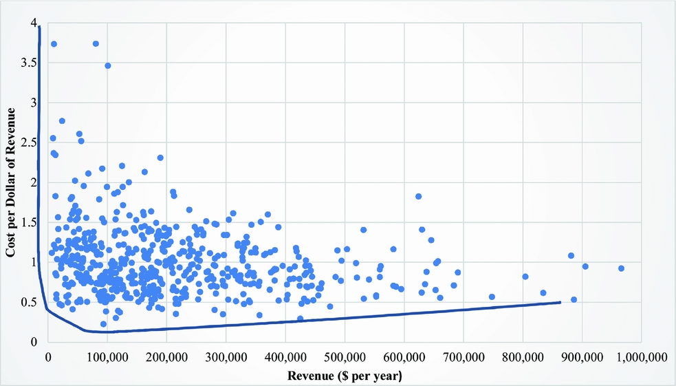
Figure 3. Western Great Plains Average Cost
Table 7. Average Reduction of InputsFootnote a for Achieving the Highest Technical Efficiency (TEVRS) for Inefficient Farms ($/producer)

a Average reduction of inputs to achieve the highest technical efficiency under variable returns to scale (TEVRS) was based on average revenue $219,473 with 1,955 acres cropped.
Note: The number of farms is on average 124 out of 141 farms that were technically inefficient in 2002–2005.
Consistent with our results, previous studies have found that modest to large farms were relatively more technically and/or economically efficient than smaller farms, including Illinois grain farmers, California fruit and vegetable producers, California dairies, and U.S. corn producers (Featherstone, Langemeier, and Ismet, Reference Featherstone, Langemeier and Ismet1997; Garcia, Sonka, and Yoo, Reference Garcia, Sonka and Yoo1982; Hall and LeVeen, Reference Hall and LeVeen1978; Matulich, Reference Matulich1978; Mugera and Langemeier, Reference Mugera and Langemeier2011; Paul et al., Reference Paul, Nehring, Banker and Somwaru2004; Weersink, Turvey, and Godah, Reference Weersink, Turvey and Godah1990). Much of this efficiency gain can be attributed to pecuniary economies of scale. Larger farms spread fixed costs of farm machinery over more acres than their smaller counterparts, reducing unit fixed costs; have greater access to financial capital; and are better poised to harbor risk. Machinery has enabled larger farms with a comparative advantage in per acre production costs and over time accumulation of expanded land holdings, notably among U.S. corn producers (Paul et al., Reference Paul, Nehring, Banker and Somwaru2004). Household labor also tends to be better used with greater demand and fewer, shorter periods of slack labor. Likewise, our finding that small farms are more scale efficient than larger farms is similar to previous studies. Byrnes et al. (Reference Byrnes, Fare, Grosskopf and Kraft1987) found that small Illinois grain farms were more scale efficient than large Illinois grain farms. In a sample of Kansas farms, Mugera and Langemeier (Reference Mugera and Langemeier2011) also found that small farms were more scale efficient than large-sized farms.
Renting land had a positive effect on all of the efficiency measures. Our modeling results imply that renting land may have allowed managers to utilize existing equipment over a larger production base increasing EE through pecuniary benefits. Although the overall effect of renting land was positive in our study, Giannakas, Schoney, and Tzouvelekas (Reference Giannakas, R and Tzouvelekas2001) identified short-term lease agreements and subsequent lack of incentives to maintain adequate agronomic conditions as having a negative effect on TE. Land tenure agreements, because they tend to be of short duration, can have a negative effect on efficiency by reducing incentives to adequately maintain agronomic conditions (Giannakas, Schoney, and Tzouvelekas Reference Giannakas, R and Tzouvelekas2001). Results from the WGP suggest that the positive aspects of having a larger land base to earn income and acquire a larger machinery complement outweigh any effect of land tenure arrangements.
Custom work had a positive effect on TE indicating it has been effective in freeing up labor to perform other operations. Its negative effect on AE, however, suggests that the costs of custom hired operations are higher than the costs of performing them using farm-owned equipment and labor. Although producers were able to improve input efficiency, there was not an overall cost savings as custom work did not have a significant effect on EE. It is also possible that managers who rely on custom work are more likely to be part-time farmers and have off-farm employment and less experience, time, and ability to allocate inputs and are less efficient than full-time managers.
5. Concluding Remarks
This article estimated the TE and EE of wheat farms in the WGP, one of the most important wheat producing regions in the United States. Our results found that wheat producers in the WGP were best able to size their farms to the optimal scale level. SE averaged 0.90, one of the highest scores reported in the agriculture production literature. Small farms were the most scale efficient reducing concerns that the agriculture sector would further concentrate and push out the smaller farms. The smaller-sized farms are operating very close to or at their optimal level of scale with nearly all farms producing under either IRS or CRS. The smaller farms should be able to increase efficiency at their current size by making better input choices. Larger farms should be encouraged to scale back their operating size to improve efficiency.
Producers were modestly efficient in their application of production inputs and resource use. TE averaged 0.65, which is in general correspondence with the performance of wheat, corn, and dairy producers found in prior studies. This reduces concerns that the less profitable wheat producing areas such as the WGP, where less new technology has been introduced, would struggle to maintain input use efficiency with other producing regions.
Results suggest concerns, however, over the ability of farms in the WGP to optimally choose inputs in response to price signals. EE averaged 0.34, substantially lower than TE and SE. Such inefficient use of resources had severe corresponding economic consequences. Our results found that if inputs and resources were efficiently applied, then production costs would be reduced by an average of $99,500 per year. Using Koopmans's efficiency modeling approach, fertilizer expenditures were identified as the primary source of inefficiency, followed by expenditures on chemicals and seeds. Policy makers and stakeholders should consider promoting new technology such as precision agriculture that can improve input use efficiency. Sensor-based technology can target fertilizer applications to site-specific locations and adjust fertilizer rates in real time based on response to plant growth. Based on the inefficient use of fertilizer, it is likely that farms are using field-level fertilizer application rates that are inadequate to account for the spatial variability in agronomic conditions and plant growth characteristics.
The increased opportunities to diversify crops over the past couple of decades have a significant and negative effect on TE and EE. Our results suggest that the introduction of crops such as sorghum and millet into the wheat rotation have not had a complementary effect on either production or economic outcomes. Further research will be needed to investigate whether the alternative crops have had unintended agronomic consequences such as promoting the spread of foliar diseases and increased weed and insect populations. Diversified farms are likely to be more innovative and entrepreneurial than the farms in the more traditional wheat monoculture, with the former more adept at planning and strategy and the later having more experience managing the technical aspects of wheat production. Producers remaining in the wheat monoculture likely have much more experience in growing wheat compared with the more diversified farms that have less familiarity growing the alternative crops. Although our data were not extensive enough to determine if there has been a learning curve associated with the alternative crops, future research using a follow-up survey could be conducted to investigate the long-term effect of diversification on efficiency and whether the efficiency of alternative crops can be improved.
Renting land had an overall positive effect on efficiency. Although SE was negatively influenced by renting land, its influence was compensated by the larger combined gains of TE, AE, and EE. Farms rent land to increase their scale of operation, seeking the pecuniary benefits from a larger farm size and corresponding efficiency gains. It appears that farm managers have largely been successful in making more efficient use of their resources and have obtained the required knowledge and experience to manage and plan larger farm sizes. Given the increase in EE, model results suggest that cash rental rates are competitively priced. There appears to be a trend, however, that renting enables farms to expand too rapidly resulting in scale inefficiency. Policy makers and stakeholders should thus encourage the use of renting land, while assisting producers in identifying their optimal farm size to improve SE.
Custom work had mixed effects on efficiency. TE was enhanced by custom work, suggesting that custom work was effectively performed in a timely manner without any significant loss in yield. It is likely that custom work enhanced TE by reducing labor bottlenecks and other production constraints, granting producers additional flexibility in other operations, particularly on diverse crop farms. It is also possible that custom work was performed in a more effective manner, perhaps through improved technology used by custom operators or field operations that were completed faster. However, the lack of a positive relationship with EE shows custom work was likely more expensive than owner-operator costs. Policy makers and researchers should consider conducting a survey of custom operator costs to identify how competitive the custom operators are in the WGP.
Future research is needed to more thoroughly investigate a couple of results that were difficult to explain. One was the significant differences in efficiency scores among the states. Researchers should consider conducting additional field studies in these states to better explain the variability. This might include a more detailed look at the inputs and technology used in each of the states as well as including an expanded scope of agricultural enterprises such as livestock. Climate, soils, and other agronomic factors could provide additional explanatory power. A second area could address identifying additional farm manager attributes to explain their performance, variables that were not present in our study because of data limitations. Only one farm manager characteristic, education, was found to be significant in the Tobit model. It is likely that the farm managers in the survey had similar backgrounds and not enough diversity to explain efficiency measures. Future researchers could include a farm survey with an expanded range of farm manager characteristics. For example, previous studies have found variables such as debt-asset ratios, capital borrowing, and access to extension information services as significant determinants of efficiency.
Appendix
Table A1. Comparison of Findings from U.S. Department of Agriculture (USDA) Estimates of Wheat Cost and Returns for the USDA Prairie Gateway Region, 2002–2005, with Average Findings from the Study Survey for States Included in Both Estimates


 Open access