


1. Introduction
The problem of particle motion in a fluid membrane was originally motivated by diffusion of proteins and lipid molecules in biological membranes separating aqueous phases (Saffman & Delbrück Reference Saffman and Delbrück1975). In his pioneering work, Saffman (Reference Saffman1976) modelled the membrane as an incompressible film (say of width  $h$) of a non-isotropic viscous fluid (say of Newtonian viscosity $\mu _m$), with no variations of fluid velocity across it; the diffusing biological molecule was modelled as a cylindrical particle of radius $a$ and height $h$. Assuming that the unbounded substrates separated by the membrane are viscous liquids (viscosity $\mu$), the dimensionless problem depends upon a single parameter, namely the Boussinesq number
 \begin{equation} {\textit{Bq}} = \frac{h \mu_m}{a\mu}. \end{equation}
The analysis of Saffman (Reference Saffman1976) involves  $h$ and $\mu _m$ only through the product $h \mu _m$. It is therefore equivalent to one involving a zero-thickness film with a Boussinesq–Scriven rheology (Scriven Reference Scriven1960) quantified by the surface viscosity $\mu _s = h \mu _m$. In what follows we employ that modern description, where the superfluous dependence upon $h$ is eliminated. The flow problem remains essentially the same if one considers, for simplicity, a single liquid substrate. We refer hereafter to that simplified scenario.
Making use of the underlying linear structure of the viscous flow problem, Saffman (Reference Saffman1976) represented the flow field via Hankel transforms. The constraint of surface incompressibility enforces a substrate flow in planes parallel to the film, with a uniform substrate pressure. The boundary conditions at the film provide dual integral equations governing the kernel of the transforms, with  ${\textit {Bq}}$ appearing as a parameter. Rather than solving the general problem, Saffman (Reference Saffman1976) focused on a translating disk in the limit ${\textit {Bq}}\to \infty$, corresponding to relatively large surface viscosity. That limit is singular, since neglecting the action of the substrate stresses on the film readily leads to the Stokes paradox.
It is well known that the Stokes paradox can be resolved by accounting for the role of inertia at distances comparable to the ratio of the kinematic viscosity to the particle speed (Leal Reference Leal2007). Given the minute particle velocities in diffusion experiments, however, these distances exceed those where other regularisation mechanisms become relevant. In particular, Saffman (Reference Saffman1976) noted that the (presumably small) substrate stresses become comparable to the film stresses at distances of order  $\mu _s/\mu (={\textit {Bq}}\,a)$. Making use of the method of matched asymptotic expansions, Saffman (Reference Saffman1976) obtained his celebrated drag approximation (see (1.2)). The comparable rotational problem in the limit ${\textit {Bq}}\to \infty$ is rather straightforward, since the two-dimensional (2-D) problem of a circular disk rotating in an unbounded viscous domain is well posed, the flow simply being a rotlet (Pozrikidis Reference Pozrikidis2011).
With the goal of extending Saffman's work to arbitrary values of  ${\textit {Bq}}$, Hughes, Pailthorpe & White (Reference Hughes, Pailthorpe and White1981) solved the dual integral equations directly. While not of the ‘standard form’ (Sneddon Reference Sneddon1966), they can be reduced to a single integral equation, which may be solved in a semianalytic manner, eventually leading to an infinite set of algebraic equations that depend upon ${\textit {Bq}}$. The main quantity of interest is the drag $D$ on the disk (normalised by the product of $\mu a$ with the disk velocity); it is a function of ${\textit {Bq}}$ alone.
Degenerating the resulting equations to the limit  ${\textit {Bq}}\to \infty$, Hughes et al. (Reference Hughes, Pailthorpe and White1981) reproduced Saffman's result (for a single substrate),
 \begin{equation} D \sim \frac{4{\rm \pi}{\textit{Bq}}}{\ln(2{\textit{Bq}})-\gamma_{E}}, \end{equation}
wherein  $\gamma _E$ is the Euler–Mascheroni constant. In the other extreme of an inviscid surface, one might have expected to retrieve the well-known drag value
 \begin{equation} D= \tfrac{16}{3}, \end{equation}
for a disk moving within a free surface. By symmetry, this value must be half the drag on a disk moving edgewise within an unbounded fluid, a classical problem that has been calculated using various methods (Ray Reference Ray1936; Lamb Reference Lamb1945; Tanzosh & Stone Reference Tanzosh and Stone1996). However, Hughes et al. (Reference Hughes, Pailthorpe and White1981) found the drag to be  $50\,\%$ larger,
 \begin{equation} \lim_{{Bq}\to0}D = 8. \end{equation}
 Hughes et al. (Reference Hughes, Pailthorpe and White1981) wrote that ‘The discrepancy … is further evidence of the singular nature of the translational problem in that even in the limit that the membrane becomes infinitely thin, it continues to influence the flow fields in the surrounding infinite fluid media’. However, other than pointing to the difference between the free-surface drag (1.3) and the small- ${\textit {Bq}}$ drag (1.4), no actual singularity was exposed.
In the literature following Hughes et al. (Reference Hughes, Pailthorpe and White1981), the difference between (1.3) and (1.4) is attributed to the need to impose surface incompressibility in the inviscid limit, a requirement absent in the case of a free surface (Fischer Reference Fischer2004a; Stone & Masoud Reference Stone and Masoud2015; Manikantan & Squires Reference Manikantan and Squires2020). While surface incompressibility is indeed the underlying source of that difference, the technical nature of the singular limit  ${\textit {Bq}}\to 0$ has remained unclear. In fact, naïvely setting ${\textit {Bq}}=0$ in the governing equations (see below) results in an ill-posed problem. Indeed, when the constraint of surface incompressibility is relaxed, that leading-order problem admits a unique solution, namely the flow leading to (1.3); that solution does not satisfy surface incompressibility, which would over-specify the flow problem.
We here revisit the translation problem using an asymptotic modus operandi. Thus, rather than analysing the dual integral equations at the limit  ${\textit {Bq}}\to 0$, we address the singular limit ${\textit {Bq}}\to 0$ from the outset. The goal is threefold. The first is to illuminate the mechanistic nature of the limit ${\textit {Bq}}\to 0$. The second is to rederive (1.4) directly, from the solution in that limit. The third is to go beyond the inviscid limit and obtain the leading-order correction to (1.4). Beyond the fundamental interest, the small- ${\textit {Bq}}$ limit is of practical value for relatively large objects (Sickert, Rondelez & Stone Reference Sickert, Rondelez and Stone2007) and highly viscous substrates (Vaz et al. Reference Vaz, Stümpel, Hallmann, Gambacorta and De Rosa1987). More generally, the understanding of particle motion within membranes may help in the interpretation of experimental results obtained from modern rheometers that use surface probes to measure interfacial viscosities (Prasad, Koehler & Weeks Reference Prasad, Koehler and Weeks2006; Zell et al. Reference Zell, Nowbahar, Mansard, Leal, Deshmukh, Mecca, Tucker and Squires2014).
We note that the Boussinesq–Scriven modelling (Scriven Reference Scriven1960) of the membrane as an incompressible viscous interface – the modern version of Saffman's description – coincides with that of a monolayer of insoluble surfactants (‘Langmuir monolayer’) in the limit of infinite Marangoni number (Manikantan & Squires Reference Manikantan and Squires2020). In that limit the description is purely mechanical, with no need to address the underlying surfactant concentration. In what follows, we shall use the notation ‘Langmuir film’ and ‘Langmuir monolayer’ interchangeably when referring to the viscous membrane.
The paper is arranged as follows. In the next section we formulate the problem, discuss the apparent incompatibility at  ${\textit {Bq}}=0$, and derive a representation for the drag in terms of the far-field behaviour of the pertinent fields. In § 3 we extract certain simplifications of the problem, valid for all ${\textit {Bq}}$. In § 4 we address the inviscid limit ${\textit {Bq}}\to 0$, obtaining an appropriate set of dual integral equations. These are solved in closed form, thus providing the velocity field as an explicit Hankel transform. The associated drag (1.4) is derived using several alternative methods. In § 5 we go beyond the inviscid limit, formulating the problem for the leading-order flow correction. Following a failed attempt to obtain the associated $\operatorname {ord}({\textit {Bq}})$ drag correction via a naïve use of the reciprocal theorem, we identify a breakdown of the asymptotic expansion near the edge of the disk. The analysis of the near-edge region is carried out in § 6. A careful reciprocal scheme, tailored to the asymptotic topology of the problem, is carried out in § 7, yielding both $\operatorname {ord}({\textit {Bq}}\ln {\textit {Bq}})$ and $\operatorname {ord}({\textit {Bq}})$ drag corrections. We conclude in § 8, describing the rotational problem which will be analysed in Part 2 of this work.
2. Problem formulation
2.1. Physical problem
The system comprises an incompressible Langmuir film that is bounding an infinite viscous substrate (viscosity  $\mu$) on one side and air on the other. The surface rheology of the film is described by the Boussinesq–Scriven model (Scriven Reference Scriven1960), with a uniform surface viscosity $\mu _s$.
A rigid disk (radius  $a$) is embedded in the film. Our goal is the calculation of the hydrodynamic drag experienced by the disk as it translates with velocity $\mathcal {U}$. We neglect the dynamical effect of the air and the deformation of the film. Dimensional arguments then imply that the ratio of the drag to $\mu \,\mathcal {U} a$ can only depend upon the Boussinesq number,
 \begin{equation} {\textit{Bq}} = \frac{\mu_s}{a\mu}. \end{equation}
2.2. Dimensionless formulation
We employ a dimensionless notation using  $a$ and $\mathcal {U}$ as length and velocity scales, respectively. The substrate stresses, and in particular the pressure, are normalised by $\mu \,\mathcal {U} / a$. The surface stresses, and in particular the surface pressure, are normalised by $\mu _s \,\mathcal {U} / a$. We utilise cylindrical coordinates
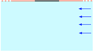
  $(\rho,\phi,z)$ in a comoving frame with the origin coinciding with the disk centre, see figure 1. The plane $z=0$ coincides with the monolayer, with $z>0$ being the liquid substrate. The upstream direction is $\phi =0$. The radial unit vector $\hat {\boldsymbol {e}}_\rho$ at that angle is denoted by $\hat {\boldsymbol {\imath }}$. (Henceforth, the unit vector associated with a generic coordinate $q$ is denoted by $\hat {\boldsymbol {e}}_q$.)

Figure 1. Schematic of the problem geometry and the  $(\rho,\phi,z)$ coordinates: (a) ‘side’ view; (b) ‘bottom’ view.
The continuity and Stokes equations governing the substrate velocity  $\boldsymbol {u}$ and pressure $p$ therefore read
 \begin{equation} \boldsymbol{\nabla} \boldsymbol{\cdot} \boldsymbol{u} = 0, \quad \boldsymbol{\nabla} \boldsymbol{\cdot} \boldsymbol{\sigma} = \boldsymbol{0} \quad \text{for} \ z>0, \end{equation}
where
 \begin{equation} \boldsymbol{\sigma} =-p \boldsymbol{\mathsf{I}} + \boldsymbol{\nabla}\boldsymbol{u} + (\boldsymbol{\nabla}\boldsymbol{u})^{{\dagger}} \end{equation}
is the Newtonian stress in the substrate, with  ${{\dagger}}$ denoting tensor transposition. They are subject to the streaming condition
 \begin{equation} \boldsymbol{u} \to -\hat{\boldsymbol{\imath}} \quad \text{as} \ \rho^2+z^2\to\infty \quad (z>0), \end{equation}
and the boundary conditions at  $z=0$, namely no-slip on the disk
 \begin{equation} \boldsymbol{u} = \boldsymbol{0} \quad \text{for} \ \rho<1, \end{equation}
and velocity continuity at the interface,
 \begin{equation} \boldsymbol{u} = \boldsymbol{u}_s \quad \text{for} \ \rho>1. \end{equation}
We note that the impermeability condition,
 \begin{equation} \hat{\boldsymbol{e}}_z \boldsymbol{\cdot} \boldsymbol{u} = 0 \quad \text{at} \ z=0, \end{equation}
is trivially satisfied.
The surface velocity  $\boldsymbol {u}_s$ at $z=0$ is governed by the incompressibility constraint
 \begin{equation} \boldsymbol{\nabla}_s \boldsymbol{\cdot} \boldsymbol{u}_s = 0 \quad \text{for} \ \rho>1 \end{equation}
and the momentum balance
 \begin{equation} \boldsymbol{\mathsf{I}}_s\boldsymbol{\cdot} \left. \boldsymbol{\sigma} \right|_{z=0^+}\boldsymbol{\cdot}\hat{\boldsymbol{e}}_z + {\textit{Bq}} \boldsymbol{\nabla}_s \boldsymbol{\cdot} \boldsymbol{\sigma}_s = \boldsymbol{0} \quad \text{for} \ \rho>1. \end{equation}
Here,  $\boldsymbol{\mathsf{I}}_s=\boldsymbol{\mathsf{I}} - \hat {\boldsymbol {e}}_z\hat {\boldsymbol {e}}_z$ is the surface idemfactor (which acts here as a projection operator), $\boldsymbol {\nabla }_s = \boldsymbol{\mathsf{I}}_s \boldsymbol {\cdot } \boldsymbol {\nabla }$ is the surface gradient operator, and the surface stress $\boldsymbol {\sigma }_s$ possesses a Newtonian form
 \begin{equation} \boldsymbol{\sigma}_s =-p_s \,\boldsymbol{\mathsf{I}}_s + \boldsymbol{\nabla}_s \boldsymbol{u}_s + (\boldsymbol{\nabla}_s \boldsymbol{u}_s)^{{\dagger}} , \end{equation}
wherein  $p_s$ is the surface pressure.
The flow field is fully determined by (2.2a,b)–(2.9). It follows from conditions (2.5) that the surface velocity must satisfy the no-slip condition
 \begin{equation} \boldsymbol{u}_s = \boldsymbol{0} \quad \text{at} \ \rho=1. \end{equation}
It also follows from (2.4) and (2.5b) that it satisfies the streaming condition
 \begin{equation} \boldsymbol{u}_s\to-\hat{\boldsymbol{\imath}} \quad \text{as} \ \rho\to\infty. \end{equation}
2.3. Surface pressure rescaling
Naïvely, the limit of an inviscid monolayer may be obtained by simply setting  ${\textit {Bq}}=0$. Then, the surface balance (2.8) becomes, using (2.3),
 \begin{equation} \boldsymbol{\mathsf{I}}_s\boldsymbol{\cdot} \left. \frac{\partial{\boldsymbol{u}}}{\partial{z}} \right|_{z=0^+} = \boldsymbol{0} \quad \text{for} \ \rho>1. \end{equation}
This shear-free condition, together with (2.4)–(2.5a), uniquely determines the solution of the Stokes equations (2.2a,b), reproducing the familiar description of a disk moving in a clean interface (Happel & Brenner Reference Happel and Brenner1965). That solution, however, when projected onto the interface via (2.5b), does not satisfy interfacial incompressibility (2.7).
The above impasse highlights the anomalous nature of the limit  ${\textit {Bq}}\to 0$. The resolution to it has to do with the scaling of the surface pressure. We conjecture that it actually becomes $\operatorname {ord}({\textit {Bq}}^{-1})$ large, balancing substrate stresses in (2.8). We therefore write
 \begin{equation} p_s = {\textit{Bq}}^{-1} \tilde p. \end{equation}
Given constraint (2.5b), no such amplification applies to the viscous surface stresses. Thus, with  $\boldsymbol {\nabla }_s\boldsymbol {u}_s=O(1)$, the viscous-stress contribution to (2.8) remains $O({\textit {Bq}})$. The rescaling (2.13) represents a normalisation of the surface pressure by the substrate scale $\mu \,\mathcal {U}$. The original normalisation by $\mu _s \,\mathcal {U} / a$, natural for both ${\textit {Bq}}=\operatorname {ord}(1)$ and ${\textit {Bq}}\gg 1$, is ill-suited for the limit ${\textit {Bq}}\to 0$.
Consistently with (2.13) we also write
 \begin{equation} \boldsymbol{\sigma}_s = {\textit{Bq}}^{-1} \tilde{\boldsymbol{\sigma}}, \end{equation}
whereby (2.8) becomes
 \begin{equation} \boldsymbol{\mathsf{I}}_s\boldsymbol{\cdot} \left. \boldsymbol{\sigma} \right|_{z=0^+}\boldsymbol{\cdot}\hat{\boldsymbol{e}}_z + \boldsymbol{\nabla}_s \boldsymbol{\cdot} \tilde{\boldsymbol{\sigma}} = \boldsymbol{0} \quad \text{for} \ \rho>1, \end{equation}
wherein (cf. (2.9))
 \begin{equation} \tilde{\boldsymbol{\sigma}} =- \tilde{p} \boldsymbol{\mathsf{I}}_s + {\textit{Bq}}[\boldsymbol{\nabla}_s \boldsymbol{u}_s + (\boldsymbol{\nabla}_s \boldsymbol{u}_s)^{{\dagger}}]. \end{equation}
2.4. Drag
The problem symmetry implies that the hydrodynamic force on the disk is antiparallel to the direction of motion. Consequently, the drag force acts in the negative- $\hat {\boldsymbol {\imath }}$ direction. Denoting the drag magnitude (normalised by $\mu \, \mathcal {U} a$) by $D$, we therefore have
 \begin{equation} \boldsymbol{\mathsf{I}}_s\boldsymbol{\cdot} \int_{\rho < 1} \left. \boldsymbol{\sigma} \right|_{z=0^+} \boldsymbol{\cdot} \hat{\boldsymbol{e}}_z \, \mathrm{d} A + \oint_{\rho=1^+} \tilde{\boldsymbol{\sigma}}\boldsymbol{\cdot} \hat{\boldsymbol{e}}_\rho \,\mathrm{d} l =- \hat{\boldsymbol{\imath}} D, \end{equation}
where the first integral is evaluated over the disk ‘bottom’ ( $z=0^+$) while the second is carried over its perimeter, $\mathrm {d} l$ being a differential length element. Equivalently,
 \begin{equation} D =-\hat{\boldsymbol{\imath}}\boldsymbol{\cdot} \int_{\rho < 1} \left. \boldsymbol{\sigma} \right|_{z=0^+} \boldsymbol{\cdot} \hat{\boldsymbol{e}}_z \, \mathrm{d} A - \hat{\boldsymbol{\imath}} \boldsymbol{\cdot} \oint_{\rho=1^+} \tilde{\boldsymbol{\sigma}}\boldsymbol{\cdot} \hat{\boldsymbol{e}}_\rho \, \mathrm{d} l . \end{equation}
 In what follows, we derive an alternative expression for  $D$, involving the flow behaviour at large distances. We start by integrating (2.15) over the annular domain $1<\rho <\varLambda$, for a fixed $\varLambda >1$. Using the 2-D variant of the divergence theorem, we obtain
 \begin{equation} \boldsymbol{\mathsf{I}}_s\boldsymbol{\cdot} \int_{1 < \rho < \varLambda} \left. \boldsymbol{\sigma} \right|_{z=0^+}\boldsymbol{\cdot}\hat{\boldsymbol{e}}_z \, \mathrm{d} A + \left(\oint_{\rho=\varLambda}-\oint_{\rho=1^+}\right)\tilde{\boldsymbol{\sigma}} \boldsymbol{\cdot} \hat{\boldsymbol{e}}_\rho \, \mathrm{d} l = \boldsymbol{0} \quad \text{for} \ \rho>1. \end{equation}
Multiplying by  $\hat {\boldsymbol {\imath }}$ and subtracting from (2.18) yields
 \begin{equation} D =-\hat{\boldsymbol{\imath}}\boldsymbol{\cdot} \int_{\rho < \varLambda} \left. \boldsymbol{\sigma} \right|_{z=0^+} \boldsymbol{\cdot} \hat{\boldsymbol{e}}_z \, \mathrm{d} A - \hat{\boldsymbol{\imath}} \boldsymbol{\cdot} \oint_{\rho=\varLambda} \tilde{\boldsymbol{\sigma}} \boldsymbol{\cdot} \hat{\boldsymbol{e}}_\rho \, \mathrm{d} l , \end{equation}
where the first integral is evaluated over the ‘bottom’ ( $z=0^+$) of the $z=0$-plane.
At this point we introduce the surface  $\mathcal {S}_\varLambda$, a hemisphere ( $z>0)$ of radius $\varLambda$ centred about the origin. Making use of (2.2b) and the divergence theorem, transforms (2.20) to
 \begin{equation} D =-\hat{\boldsymbol{\imath}}\boldsymbol{\cdot} \int_{\mathcal{S}_\varLambda} \boldsymbol{\sigma} \boldsymbol{\cdot} \hat{\boldsymbol{e}}_r \, \mathrm{d} A - \hat{\boldsymbol{\imath}} \boldsymbol{\cdot} \oint_{\rho=\varLambda} \tilde{\boldsymbol{\sigma}} \boldsymbol{\cdot} \hat{\boldsymbol{e}}_\rho \, \mathrm{d} l , \end{equation}
wherein  $\hat {\boldsymbol {e}}_r$ is a unit vector in the radial direction. Since $\varLambda$ is at our disposal, it can be taken to be arbitrarily large. The drag representation (2.21) then depends only upon the asymptotic behaviour of the substrate and surface stresses at large distances.
3. Simplifications
3.1. General
Using (2.3) and (2.6), it is readily seen that
 \begin{equation} \boldsymbol{\sigma} \boldsymbol{\cdot} \hat{\boldsymbol{e}}_z =-p \,\hat{\boldsymbol{e}}_z + \frac{\partial{\boldsymbol{u}}}{\partial{z}} \quad \text{at} \ z=0. \end{equation}
The interfacial momentum balance (2.15) therefore simplifies to
 \begin{equation} \boldsymbol{\mathsf{I}}_s\boldsymbol{\cdot} \left. \frac{\partial{\boldsymbol{u}}}{\partial{z}} \right|_{z=0^+} + \boldsymbol{\nabla}_s \boldsymbol{\cdot} \tilde{\boldsymbol{\sigma}} = \boldsymbol{0} \quad \text{for} \ \rho>1, \end{equation}
while the drag expression (2.18) becomes
 \begin{equation} D =-\hat{\boldsymbol{\imath}}\boldsymbol{\cdot} \int_{\rho<1} \left. \frac{\partial{\boldsymbol{u}}}{\partial{z}} \right|_{z=0^+} \, \mathrm{d} A - \hat{\boldsymbol{\imath}} \boldsymbol{\cdot} \oint_{\rho=1^+} \tilde{\boldsymbol{\sigma}} \boldsymbol{\cdot} \hat{\boldsymbol{e}}_\rho \, \mathrm{d} l . \end{equation}
 In fact, both (3.2) and (3.3) may be written in terms of substrate velocity  $\boldsymbol {u}$. Thus, making use of (2.5b), (2.7) and (2.16), (3.2) becomes
 \begin{equation} \boldsymbol{\mathsf{I}}_s\boldsymbol{\cdot} \frac{\partial{\boldsymbol{u}}}{\partial{z}} - \boldsymbol{\nabla}_s \tilde{p} + {\textit{Bq}} \nabla_s^2 \boldsymbol{u} = \boldsymbol{0} \quad \text{for}\ \rho>1, \end{equation}
when it is understood that both  $\boldsymbol {u}$ and $\partial \boldsymbol {u}/\partial z$ are evaluated at $z=0$. Similarly, making use of (2.5b) and (2.16), (3.3) becomes
 \begin{equation} D =-\hat{\boldsymbol{\imath}}\boldsymbol{\cdot} \int_{\rho<1} \frac{\partial{\boldsymbol{u}}}{\partial{z}}\, \mathrm{d} A +\hat{\boldsymbol{\imath}} \boldsymbol{\cdot} \oint_{\rho=1^+} \hat{\boldsymbol{e}}_\rho \,\tilde{p} \, \mathrm{d} l - {\textit{Bq}} \, \hat{\boldsymbol{\imath}} \boldsymbol{\cdot} \oint_{\rho=1^+} [\boldsymbol{\nabla}_s\boldsymbol{u} + (\boldsymbol{\nabla}_s\boldsymbol{u})^{{\dagger}}] \boldsymbol{\cdot} \hat{\boldsymbol{e}}_\rho \, \mathrm{d} l . \end{equation}
With the surface velocity absent in (3.4)–(3.5), it only appears in (2.7).
3.2. Flow in parallel planes
In the analysis of equivalent problems (Saffman Reference Saffman1976; Hughes et al. Reference Hughes, Pailthorpe and White1981), it was rigorously shown that the constraint of surface incompressibility eventually necessitates a flow structure where  $\boldsymbol {u}$ has no component in the $z$-direction. Following Stone & Ajdari (Reference Stone and Ajdari1998) we elect here to follow a simplified path, where we postulate that the substrate flow has no $z$-component. Then, substrate incompressibility (2.2a) readily implies that surface incompressibility (2.7) is trivially satisfied. In particular, the surface velocity $\boldsymbol {u}_s$ no longer appears in the governing equations.
The restriction of fluid motion to parallel planes has two immediate consequences. First, we can omit the projection operator in (3.4). Second, with (2.2a,b) necessitating pressure gradients which are independent of  $z$, it follows from (2.4) that $p$ is uniform throughout. Thus, the stress is purely deviatoric (cf. (2.3)),
 \begin{equation} \boldsymbol{\sigma} = \boldsymbol{\nabla}\boldsymbol{u} + (\boldsymbol{\nabla}\boldsymbol{u})^{{\dagger}}, \end{equation}
and the Stokes equations (2.2b) simply read
 \begin{equation} \nabla^2\boldsymbol{u} = \boldsymbol{0} \quad \text{for} \ z>0. \end{equation}
3.3. Symmetries
It follows from the problem symmetry that the substrate velocity possesses the form
 \begin{equation} \boldsymbol{u} = \hat{\boldsymbol{e}}_\rho u_\rho(\rho,z) \cos\phi + \hat{\boldsymbol{e}}_\phi u_\phi(\rho,z) \sin\phi. \end{equation}
The surface pressure is then
 \begin{equation} \tilde p(\rho,\phi) = \varPi(\rho) \cos\phi. \end{equation}
With the aforementioned structure, the continuity equation (2.2a) becomes
 \begin{equation} \frac{\partial{}}{\partial{\rho}}(\rho u_\rho)+u_\phi=0, \end{equation}
while the  $\rho$- and $\phi$-components of the Stokes equations (3.7) give
 $$\begin{gather} \frac{\partial{^2u_\rho}}{\partial{z^2}} + \frac{\partial{^2u_\rho}}{\partial{\rho^2}} + \frac{1}{\rho} \frac{\partial{u_\rho}}{\partial{\rho}} -2\frac{u_\rho+u_\phi}{\rho^2} = 0, \end{gather}$$
 $$\begin{gather}\frac{\partial{^2u_\phi}}{\partial{z^2}} +\frac{\partial{^2u_\phi}}{\partial{\rho^2}} + \frac{1}{\rho} \frac{\partial{u_\phi}}{\partial{\rho}} -2\frac{u_\rho+u_\phi}{\rho^2}=0. \end{gather}$$
The variables  $u_\rho$ and $u_\phi$ are subject to the streaming condition (cf. (2.4))
 \begin{equation} u_\rho\to -1,\quad u_\phi \to 1 \quad \text{as} \ \rho^2+z^2\to\infty \quad (z>0). \end{equation}
At  $z=0$, the no-slip condition (2.5a) becomes
 \begin{equation} u_\rho= u_\phi=0 \quad \text{for} \ \rho<1, \end{equation}
while the  $\rho$- and $\phi$-components of the interfacial balance (3.4) become
 $$\begin{gather} \frac{\partial{u_\rho}}{\partial{z}}- \frac{\mathrm{d}{\varPi}}{\mathrm{d}{\rho}} + {\textit{Bq}} \left( \frac{\partial{^2u_\rho}}{\partial{\rho^2}} + \frac{1}{\rho} \frac{\partial{u_\rho}}{\partial{\rho}} -2\frac{u_\rho+u_\phi}{\rho^2}\right)=0, \end{gather}$$
 $$\begin{gather}\frac{\partial{u_\phi}}{\partial{z}} +\frac{\varPi}{\rho} + {\textit{Bq}} \left( \frac{\partial{^2u_\phi}}{\partial{\rho^2}} + \frac{1}{\rho} \frac{\partial{u_\phi}}{\partial{\rho}} -2\frac{u_\rho+u_\phi}{\rho^2}\right)=0, \end{gather}$$
for  $\rho >1$.
Substitution of (3.8)–(3.9) into (3.5) followed by integration over  $\phi$ yields
 \begin{align} D = {\rm \pi}\int_0^{1^-} \left(\frac{\partial{u_\phi}}{\partial{z}}-\frac{\partial{u_\rho}}{\partial{z}}\right) \rho \, \mathrm{d} \rho + {\rm \pi}\left.\varPi\right|_{\rho=1^+} - {\rm \pi}{\textit{Bq}} \left( 2 \frac{\partial{u_\rho}}{\partial{\rho}} - \frac{\partial{u_\phi}}{\partial{\rho}} + {u_\rho+u_\phi}\right)_{\rho=1^+},\end{align}
with the understanding that both  $u_\rho$ and $u_\phi$ as well as their $z$-derivatives are evaluated at $z=0$.
4. The small- ${\textit {Bq}}$ limit

We now proceed to the limit  ${\textit {Bq}}\ll 1$, posing the generic expansion
 \begin{equation} f \sim f^{(0)} + {\textit{Bq}}\,f^{(1)} + \dots \end{equation}
for all field variables. We note that, in the problem formulation, the small parameter  ${\textit {Bq}}$ appears only in condition (3.14). Equations (3.10)–(3.13) therefore hold at any asymptotic order.
4.1. Inviscid solution
Setting  ${\textit {Bq}}=0$ in (3.14) we obtain
 \begin{equation} \frac{\partial{u_\rho^{(0)}}}{\partial{z}} = \frac{\mathrm{d}{\varPi^{(0)}}}{\mathrm{d}{\rho}}, \quad \frac{\partial{u_\phi^{(0)}}}{\partial{z}} =-\frac{\varPi^{(0)}}{\rho} \quad \text{for} \ \rho>1 . \end{equation}
By eliminating  $\varPi ^{(0)}$ we readily obtain the vorticity balance
 \begin{equation} \frac{\partial{}}{\partial{r}} \left(\rho\frac{\partial{u_\phi^{(0)}}}{\partial{z}}\right) + \frac{\partial{u_\rho^{(0)}}}{\partial{z}} = 0 . \end{equation}
The general solution of (3.10)–(3.11) that satisfies (3.12) is given in terms of Hankel transforms (Saffman Reference Saffman1976)
 $$\begin{gather} u_\rho^{(0)} +1= \tfrac{1}{2} \int_0^\infty B(k) [{\rm J}_2(k\rho)+{\rm J}_0(k\rho)] \mathrm{e}^{-kz}\, \mathrm{d} k, \end{gather}$$
 $$\begin{gather}u_\phi^{(0)} -1= \tfrac{1}{2} \int_0^\infty B(k) [{\rm J}_2(k\rho)-{\rm J}_0(k\rho)] \mathrm{e}^{-kz}\, \mathrm{d} k, \end{gather}$$
wherein  ${\rm J}_n$ is the Bessel function of the first kind. From (4.2b) we then obtain
 \begin{equation} \varPi^{(0)} = \frac{\rho}{2} \int_0^\infty k B(k) [{\rm J}_2(k\rho)-{\rm J}_0(k\rho)] \, \mathrm{d} k. \end{equation}
 We now apply the boundary conditions at  $z=0$ to the Hankel transforms (4.4). The first condition is at the interface. Substituting (4.4) into the vorticity equation (4.3) yields the integral equation
 \begin{equation} \int_0^\infty k^2 B(k) {\rm J}_1(k \rho) \, \mathrm{d} k = 0 \quad \text{for} \ \rho>1. \end{equation}
 The second equation is at the disk bottom. Substitution of (4.4) into the no-slip condition (3.13) at  $\operatorname {ord}(1)$ yields
 \begin{equation} \int_0^\infty B(k) {\rm J}_2(k \rho)\, \mathrm{d} k = 0 ,\quad \int_0^\infty B(k) {\rm J}_0(k \rho)\, \mathrm{d} k = 2, \end{equation}
for  $\rho <1$. Mutual addition of (4.7a,b), in conjunction with the identity
 \begin{equation} {\rm J}_0(x)+{\rm J}_2(x) = \frac{2}{x} {\rm J}_1(x), \end{equation}
yields the second equation governing  $B(k)$,
 \begin{equation} \int_0^\infty \frac{B(k)}{k} {\rm J}_1(k \rho)\, \mathrm{d} k = \rho \quad \text{for} \ \rho<1. \end{equation}
 The function  $B(k)$ is determined by the dual integral equations (4.6) and (4.9). Multiplying (4.9) by $\rho$ and differentiating with respect to $\rho$ gives
 \begin{equation} \int_0^\infty B(k) {\rm J}_0(k \rho)\, \mathrm{d} k = 2 \quad \text{for} \ \rho<1, \end{equation}
where we have used the identity
 \begin{equation} \frac{\mathrm{d}{{\rm J}_0}}{\mathrm{d}\kern0.06em {x}}=-{\rm J}_1(x). \end{equation}
Also, integrating (4.6) from  $\rho$ to $\infty$ and making use of (4.11) in conjunction with ${\rm J}_0(\infty )=0$ yields
 \begin{equation} \int_0^\infty k B(k) {\rm J}_0(k \rho) \, \mathrm{d} k = 0 \quad \text{for} \ \rho>1. \end{equation}
The dual set (4.10) and (4.12) is equivalent to that encountered in the classical calculation of the capacitance of an electrified disk, a problem originally solved by Weber (Reference Weber1873). In the present context we find (Sneddon Reference Sneddon1966)
 \begin{equation} B(k) =\frac{4\sin k}{{\rm \pi} k}. \end{equation}
Substitution of (4.13) into (4.5) yields the simple expression
 \begin{equation} \varPi^{(0)} = \frac{4}{{\rm \pi} \rho}. \end{equation}
No comparable closed-form for the substrate fields  $u_\rho ^{(0)}$ and $u_\phi ^{(0)}$ is obtained by substituting (4.13) into (4.4) for arbitrary $z$. Nonetheless, evaluation at $z=0$ (with $\rho >1$) gives
 \begin{align} u_\rho^{(0)} +1= \frac{2}{\rm \pi} \left(\frac{\sqrt{\rho^2-1}}{\rho^2} + \arcsin\frac{1}{\rho}\right), \quad u_\phi^{(0)} -1= \frac{2}{\rm \pi} \left(\frac{\sqrt{\rho^2-1}}{\rho^2} - \arcsin\frac{1}{\rho}\right). \end{align}
Similarly, evaluation of the derivatives at  $z=0$ (with $\rho <1$) gives
 \begin{equation} \frac{\partial{u_\rho^{(0)}}}{\partial{z}} = \frac{4}{{\rm \pi} \rho^2} \left(\sqrt{1-\rho^2}-1\right), \quad \frac{\partial{u_\phi^{(0)}}}{\partial{z}} = \frac{4}{{\rm \pi} \rho^2} \left(\frac{1}{\sqrt{1-\rho^2}} -1\right). \end{equation}
 We can also obtain the asymptotic behaviour of  $\boldsymbol {u}^{(0)}$ at large distances, $\rho ^2+z^2\to \infty$. To that end, we employ the spherical polar coordinates $(r,\theta,\phi )$, related to the present cylindrical coordinates via
 \begin{equation} z = r \cos\theta, \quad \rho = r \sin\theta. \end{equation}
In the limit  $r\to \infty$, the integral representations (4.4) are dominated by $k=O(1/r)$. We readily obtain
 \begin{equation} u_\rho^{(0)} +1\sim \frac{2}{{\rm \pi} r \cos^2(\theta/2)}, \quad u_\phi^{(0)} -1\sim-\frac{2\cos\theta}{{\rm \pi} r \cos^2(\theta/2)} \quad \text{as} \ r\to\infty. \end{equation}
Note that at  $\theta ={\rm \pi} /2$, where $r=\rho$ and $\boldsymbol {u}=\boldsymbol {u}_s$, (4.18a,b) reduces to the purely radial field
 \begin{equation} \boldsymbol{u}_s^{(0)}+\hat{\boldsymbol{\imath}}\sim \frac{4}{{\rm \pi}\rho} \hat{\boldsymbol{e}}_\rho\hat{\boldsymbol{e}}_\rho\boldsymbol{\cdot}\hat{\boldsymbol{\imath}} \quad \text{as} \ \rho\to\infty, \end{equation}
in agreement with the associated 2-D Green's function of the problem (Fischer Reference Fischer2004b).
4.2. Drag in an inviscid monolayer
We now proceed to the calculation of the drag  $D^{(0)}$, which is the quantity of interest. Here, the simplest calculation method is the direct one, using (3.15). Setting ${\textit {Bq}}=0$ we obtain
 \begin{equation} D^{(0)} = {\rm \pi}\int_0^{1^-} \left(\frac{\partial{u_\phi^{(0)}}}{\partial{z}}-\frac{\partial{u_\rho^{(0)}}}{\partial{z}}\right)\rho\,\mathrm{d} \rho + \left. {\rm \pi}\varPi^{(0)}\right|_{\rho=1^+} . \end{equation}
Substitution of (4.14) and (4.16a,b) into (4.20) yields
 \begin{equation} D^{(0)}=8, \end{equation}
where half the drag is contributed by viscous stresses on the disk bottom while the other half is due to interfacial pressure. A derivation of (4.21) using the direct formula (3.15), which does not require the explicit expressions (4.14) and (4.16a,b), is presented in Appendix A.
Alternatively, we can use representation (2.21), which at leading order gives
 \begin{equation} D^{(0)} =-\hat{\boldsymbol{\imath}}\boldsymbol{\cdot} \int_{\mathcal{S}_\varLambda} \boldsymbol{\sigma}^{(0)} \boldsymbol{\cdot} \hat{\boldsymbol{e}}_r \, \mathrm{d} A - \hat{\boldsymbol{\imath}} \boldsymbol{\cdot} \oint_{\rho=\varLambda} \tilde{\boldsymbol{\sigma}}^{(0)} \boldsymbol{\cdot} \hat{\boldsymbol{e}}_\rho \, \mathrm{d} l . \end{equation}
Noting that (see (3.6) and (2.16))
 \begin{equation} \boldsymbol{\sigma}^{(0)} = \boldsymbol{\nabla}\boldsymbol{u}^{(0)} + (\boldsymbol{\nabla}\boldsymbol{u}^{(0)})^{{\dagger}}, \quad \tilde{\boldsymbol{\sigma}}^{(0)} =- \tilde p^{(0)} \boldsymbol{\mathsf{I}}_s, \end{equation}
we see that
 \begin{equation} D^{(0)} =-\hat{\boldsymbol{\imath}}\boldsymbol{\cdot} \int_{\mathcal{S}_\varLambda} [\boldsymbol{\nabla}\boldsymbol{u}^{(0)} + (\boldsymbol{\nabla}\boldsymbol{u}^{(0)})^{{\dagger}}] \boldsymbol{\cdot} \hat{\boldsymbol{e}}_r \, \mathrm{d} A +\hat{\boldsymbol{\imath}} \boldsymbol{\cdot} \oint_{\rho=\varLambda} \hat{\boldsymbol{e}}_\rho \,\tilde{p}^{(0)} \, \mathrm{d} l . \end{equation}
The contribution of the second integral, using (3.9) and (4.14), is  $4$. In evaluating the contribution of the first integral, we exploit the independence of the drag upon the arbitrary parameter $\varLambda$, and form the limit $\varLambda \to \infty$. Substitution of (4.18a,b) yields $4$. We have therefore reproduced (4.21), where again half the drag is contributed by the interfacial pressure.
Considering the limit  $\varLambda \to \infty$, it is evident that the $1/r$ decay rate in (4.18a,b) is necessary for a finite drag contribution from viscous stresses over the hemisphere $\mathcal {S}_\varLambda$, which decay there as $1/\varLambda ^2$. We observe that (4.18a,b), which must satisfy a surface incompressibility condition at the interface $\theta ={\rm \pi} /2$, differ from the large- $r$ asymptotic limit of the classical solution of a disk in a clean interface, which is the familiar Stokeslet (corresponding to drag $16/3$).
5. Nearly inviscid film
We now proceed to calculate the drag correction  $D^{(1)}$. With the use of the reciprocal theorem in mind, we find it convenient to summarise first the equations governing the $\operatorname {ord}(1)$ problem in an invariant notation. The continuity and Stokes equations read
 \begin{equation} \boldsymbol{\nabla} \boldsymbol{\cdot} \boldsymbol{u}^{(0)} = 0, \quad \boldsymbol{\nabla} \boldsymbol{\cdot} \boldsymbol{\sigma}^{(0)} = \boldsymbol{0} \quad \text{for} \ z>0. \end{equation}
These are supplemented by the streaming condition
 \begin{equation} \boldsymbol{u}^{(0)} \to -\hat{\boldsymbol{\imath}} \quad \text{as} \ r\to\infty \quad (z>0), \end{equation}
and two conditions at  $z=0$: the first is the no-slip condition (see (2.5a)),
 \begin{equation} \boldsymbol{u}^{(0)} = \boldsymbol{0} \quad \text{for} \ \rho<1; \end{equation}
the second is the shear balance (see (2.15)),
 \begin{equation} \boldsymbol{\mathsf{I}}_s\boldsymbol{\cdot} \left. \boldsymbol{\sigma}^{(0)} \right|_{z=0^+}\boldsymbol{\cdot}\hat{\boldsymbol{e}}_z + \boldsymbol{\nabla}_s \boldsymbol{\cdot} \tilde{\boldsymbol{\sigma}}^{(0)} = \boldsymbol{0} \quad \text{for} \ \rho>1. \end{equation}
The stress expressions are given in (4.23a,b). The surface velocity is simply provided by the substrate velocity at  $z=0$ (cf. (2.5b))
 \begin{equation} \boldsymbol{u}_s^{(0)} = \boldsymbol{u}^{(0)} (z=0); \end{equation}
it satisfies surface incompressibility (cf. (2.7))
 \begin{equation} \boldsymbol{\nabla}_s \boldsymbol{\cdot} \boldsymbol{u}_s^{(0)} = 0 \quad \text{for} \ \rho>1 . \end{equation}
 The  $\operatorname {ord}({\textit {Bq}})$ balances readily follow. The continuity and Stokes equations read
 \begin{equation} \boldsymbol{\nabla} \boldsymbol{\cdot} \boldsymbol{u}^{(1)} = 0, \quad \boldsymbol{\nabla} \boldsymbol{\cdot} \boldsymbol{\sigma}^{(1)} = \boldsymbol{0} \quad \text{for} \ z>0. \end{equation}
These are supplemented by the decay condition
 \begin{equation} \boldsymbol{u}^{(1)} \to \boldsymbol{0} \quad \text{as} \ r\to\infty, \end{equation}
and two conditions at  $z=0$: the first,
 \begin{equation} \boldsymbol{u}^{(1)} = \boldsymbol{0} \quad \text{for} \ \rho<1, \end{equation}
obtained from (2.5a); and the second,
 \begin{equation} \boldsymbol{\mathsf{I}}_s\boldsymbol{\cdot} \left. \boldsymbol{\sigma}^{(1)} \right|_{z=0^+}\boldsymbol{\cdot}\hat{\boldsymbol{e}}_z + \boldsymbol{\nabla}_s \boldsymbol{\cdot} \tilde{\boldsymbol{\sigma}}^{(1)} = \boldsymbol{0} \quad \text{for} \ \rho>1, \end{equation}
obtained from (2.15). From (2.16) and (3.6) we have (cf. (4.23a,b))
 \begin{equation} \boldsymbol{\sigma}^{(1)} = \boldsymbol{\nabla}\boldsymbol{u}^{(1)} + (\boldsymbol{\nabla}\boldsymbol{u}^{(1)})^{{\dagger}}, \quad \tilde{\boldsymbol{\sigma}}^{(1)} =- \tilde{p}^{(1)} \boldsymbol{\mathsf{I}}_s + \boldsymbol{\nabla}_s \boldsymbol{u}_s^{(0)} + (\boldsymbol{\nabla}_s \boldsymbol{u}_s^{(0)})^{{\dagger}}. \end{equation}
 The associated drag correction is obtained from (2.21), which at  $\operatorname {ord}({\textit {Bq}})$ gives (cf. (4.22))
 \begin{equation} D^{(1)} =-\hat{\boldsymbol{\imath}}\boldsymbol{\cdot} \int_{\mathcal{S}_\varLambda} \boldsymbol{\sigma}^{(1)} \boldsymbol{\cdot} \hat{\boldsymbol{e}}_r \, \mathrm{d} A - \hat{\boldsymbol{\imath}} \boldsymbol{\cdot} \oint_{\rho=\varLambda} \tilde{\boldsymbol{\sigma}}^{(1)} \boldsymbol{\cdot} \hat{\boldsymbol{e}}_\rho \, \mathrm{d} l . \end{equation}
5.1. Drag correction: naïve try with the reciprocal theorem
In principle, the drag correction can be obtained using (5.12) from the solution of the problem (5.7a,b)–(5.11a,b) governing  $\boldsymbol {u}^{(1)}$ and $\tilde {p}^{(1)}$. As we want to avoid that detailed solution, we resort to the use of the reciprocal theorem (Masoud & Stone Reference Masoud and Stone2019), already employed in related problems in the field (Stone & Masoud Reference Stone and Masoud2015). Exploiting the fact that both the flow $\boldsymbol {u}^{(0)}$ (with stress $\boldsymbol {\sigma }^{(0)}$) and $\boldsymbol {u}^{(1)}$ (with stress $\boldsymbol {\sigma }^{(1)}$) satisfy the homogeneous Stokes equations, see (5.1a,b) and (5.7a,b), our starting point is (Happel & Brenner Reference Happel and Brenner1965)
 \begin{equation} \boldsymbol{\nabla} \boldsymbol{\cdot} (\boldsymbol{u}^{(0)} \boldsymbol{\cdot} \boldsymbol{\sigma}^{(1)}) = \boldsymbol{\nabla} \boldsymbol{\cdot} (\boldsymbol{u}^{(1)} \boldsymbol{\cdot} \boldsymbol{\sigma}^{(0)}). \end{equation}
We integrate (5.13) over the domain bounded by the hemisphere  $\mathcal {S}_\varLambda$ and the plane $z=0^+$. Integration of the left-hand side gives, upon making use the divergence theorem,
 \begin{equation} \int_{\mathcal{S}_\varLambda} \boldsymbol{u}^{(0)} \boldsymbol{\cdot} \boldsymbol{\sigma}^{(1)} \boldsymbol{\cdot} \hat{\boldsymbol{e}}_r\, \mathrm{d} A -\int_{0<\rho<1} \boldsymbol{u}^{(0)} \boldsymbol{\cdot} \boldsymbol{\sigma}^{(1)} \boldsymbol{\cdot}\hat{\boldsymbol{e}}_z\,\mathrm{d} A -\int_{1<\rho<\varLambda} \boldsymbol{u}^{(0)} \boldsymbol{\cdot} \boldsymbol{\sigma}^{(1)} \boldsymbol{\cdot}\hat{\boldsymbol{e}}_z\,\mathrm{d} A. \end{equation}
(In what follows, integrals over the domains  $0<\rho <1$ and $1<\rho <\varLambda$ are understood to be evaluated at $z=0^+$.) Using (5.3) and (5.10), (5.14) simplifies to
 \begin{equation} \int_{\mathcal{S}_\varLambda} \boldsymbol{u}^{(0)} \boldsymbol{\cdot} \boldsymbol{\sigma}^{(1)} \boldsymbol{\cdot} \hat{\boldsymbol{e}}_r\, \mathrm{d} A +\int_{1<\rho<\varLambda} \boldsymbol{u}^{(0)} \boldsymbol{\cdot} (\boldsymbol{\nabla}_s \boldsymbol{\cdot} \tilde{\boldsymbol{\sigma}}^{(1)})\,\mathrm{d} A. \end{equation}
 At this point we make use of (2.5b), conveniently employing the surface velocity  $\boldsymbol {u}_s^{(0)}$ instead of $\boldsymbol {u}^{(0)}$ in the second integral of (5.15). Noting that, for any surface tensor field $\boldsymbol{\mathsf{S}}$ and surface vector field $\boldsymbol {a}$,
 \begin{equation} \boldsymbol{\nabla}_s \boldsymbol{\cdot} (\boldsymbol{\mathsf{S}} \boldsymbol{\cdot} {\boldsymbol{a}}) = (\boldsymbol{\nabla}_s \boldsymbol{\cdot} \boldsymbol{\mathsf{S}}) \boldsymbol{\cdot} {\boldsymbol{a}} + \boldsymbol{\mathsf{S}}\boldsymbol{:}\boldsymbol{\nabla}_s{\boldsymbol{a}}, \end{equation}
the second integral in (5.15) becomes
 \begin{equation} \int_{1<\rho<\varLambda} [\boldsymbol{\nabla}_s \boldsymbol{\cdot} (\boldsymbol{u}_s^{(0)} \boldsymbol{\cdot} \tilde{\boldsymbol{\sigma}}^{(1)}) - \tilde{\boldsymbol{\sigma}}^{(1)} \boldsymbol{:} \boldsymbol{\nabla}_s \boldsymbol{u}_s^{(0)} ] \,\mathrm{d} A. \end{equation}
Upon making use of the surface variant of the divergence theorem and exploiting (5.3), we find that
 \begin{equation} \int_{1<\rho<\varLambda} \boldsymbol{\nabla}_s \boldsymbol{\cdot} (\boldsymbol{u}_s^{(0)} \boldsymbol{\cdot} \tilde{\boldsymbol{\sigma}}^{(1)}) \,\mathrm{d} A = \oint_{\rho=\varLambda} \boldsymbol{u}_s^{(0)} \boldsymbol{\cdot} \tilde{\boldsymbol{\sigma}}^{(1)} \boldsymbol{\cdot} \hat{\boldsymbol{e}}_\rho \, \mathrm{d} l. \end{equation}
Also, making use of (5.6) and (5.11b)
 \begin{equation} \int_{1<\rho<\varLambda} \tilde{\boldsymbol{\sigma}}^{(1)} \boldsymbol{:} \boldsymbol{\nabla}_s \boldsymbol{u}_s^{(0)} \,\mathrm{d} A = 2\int_{1<\rho<\varLambda} \boldsymbol{\mathsf{e}}^{(0)}_s \boldsymbol{:} \boldsymbol{\mathsf{e}}^{(0)}_s\,\mathrm{d} A \end{equation}
wherein
 \begin{equation} \boldsymbol{\mathsf{e}}^{(0)}_s = \tfrac{1}{2} [\boldsymbol{\nabla}_s \boldsymbol{u}_s^{(0)} + (\boldsymbol{\nabla}_s \boldsymbol{u}_s^{(0)})^{{\dagger}}], \end{equation}
is the surface rate-of-strain tensor associated with  $\boldsymbol {u}^{(0)}$.
To summarise, the volume integral of the left-hand side of (5.13) is
 \begin{equation} \int_{\mathcal{S}_\varLambda} \boldsymbol{u}^{(0)} \boldsymbol{\cdot} \boldsymbol{\sigma}^{(1)} \boldsymbol{\cdot} \hat{\boldsymbol{e}}_r\, \mathrm{d} A + \oint_{\rho=\varLambda}\boldsymbol{u}^{(0)} \boldsymbol{\cdot} \tilde{\boldsymbol{\sigma}}^{(1)} \boldsymbol{\cdot} \hat{\boldsymbol{e}}_\rho \, \mathrm{d} l - 2\int_{1<\rho<\varLambda} \boldsymbol{\mathsf{e}}^{(0)}_s \boldsymbol{:} \boldsymbol{\mathsf{e}}^{(0)}_s\,\mathrm{d} A, \end{equation}
where we reverted to the substrate velocity. In a similar manner we find that the integral of the right-hand side of (5.13) is
 \begin{equation} \int_{\mathcal{S}_\varLambda} \boldsymbol{u}^{(1)} \boldsymbol{\cdot} \boldsymbol{\sigma}^{(0)} \boldsymbol{\cdot} \hat{\boldsymbol{e}}_r\, \mathrm{d} A + \oint_{\rho=\varLambda}\boldsymbol{u}^{(1)} \boldsymbol{\cdot} \tilde{\boldsymbol{\sigma}}^{(0)} \boldsymbol{\cdot} \hat{\boldsymbol{e}}_\rho \, \mathrm{d} l. \end{equation}
 We now form the limit  $\varLambda \to \infty$. Recalling that $\boldsymbol {\sigma }^{(0)}=O(r^{-2})$ and $\tilde {\boldsymbol {\sigma }}^{(0)}=O(r^{-1})$ at large $r$, we see from (5.8) that (5.22) vanishes in that limit. From (5.2) and (5.21) we therefore obtain
 \begin{equation} -\hat{\boldsymbol{\imath}} \boldsymbol{\cdot} \lim_{\varLambda\to\infty} \left[\int_{\mathcal{S}_\varLambda} \boldsymbol{\sigma}^{(1)} \boldsymbol{\cdot} \hat{\boldsymbol{e}}_r\, \mathrm{d} A + \oint_{\rho=\varLambda} \tilde{\boldsymbol{\sigma}}^{(1)} \boldsymbol{\cdot} \hat{\boldsymbol{e}}_\rho \, \mathrm{d} l \right] - 2\int_{\rho>1} \boldsymbol{\mathsf{e}}^{(0)}_s \boldsymbol{:} \boldsymbol{\mathsf{e}}^{(0)}_s\,\mathrm{d} A = 0. \end{equation}
Since  $\varLambda$ is arbitrary in (5.12), the first term in (5.23) is $D^{(1)}$. We therefore find the drag as a surface-dissipation quadrature,
 \begin{equation} D^{(1)} = 2\int_{\rho>1} \boldsymbol{\mathsf{e}}^{(0)}_s : \boldsymbol{\mathsf{e}}^{(0)}_s\,\mathrm{d} A. \end{equation}
 Substituting (4.15a,b) in conjunction with the angular dependence (3.8) and using the expressions for the rate-of-strain components in polar coordinates (Batchelor Reference Batchelor1967) gives, upon integrating over  $\phi$,
 \begin{equation} D^{(1)} = 2{\rm \pi} \int_1^\infty \mathcal{D}(\rho)\,\mathrm{d} \rho, \end{equation}
wherein
 \begin{align} \mathcal{D} = \rho\left[\left(\frac{\partial{u_\rho^{(0)}}}{\partial{\rho}}\right)^2 + \frac{1}{2}\left(\frac{\partial{u_\phi^{(0)}}}{\partial{\rho}}\right)^2 + \frac{3}{2} \left(\frac{u_\rho^{(0)}+u_\phi^{(0)}}{\rho}\right)^2 - \frac{u_\rho^{(0)}+u_\phi^{(0)}}{\rho}\frac{\partial{u_\phi^{(0)}}}{\partial{\rho}}\right]_{z=0}. \end{align}
 While (5.24) may appear plausible, it is in fact meaningless, as the integral does not converge. Indeed, (4.15a,b) implies the following asymptotic behaviours at  $z=0$:
 \begin{equation} u_\rho^{(0)} = O\{(\rho-1)^{3/2}\} \quad \text{as} \ \rho\searrow 1 \end{equation}
and
 \begin{equation} u_\phi^{(0)} \sim \frac{4}{\rm \pi}2^{1/2}(\rho-1)^{1/2} + O\{(\rho-1)^{3/2}\} \quad \text{as}\ \rho\searrow 1. \end{equation}
Substitution into (5.26) gives
 \begin{equation} \mathcal{D}\sim \frac{4}{{\rm \pi}^2(\rho-1)} \quad \text{as} \ \rho\searrow 1. \end{equation}
With that behaviour, the integral appearing in (5.25) diverges logarithmically.
5.2. Edge singularity
Our attempt to employ the reciprocal theorem has failed because of the square-root singularity in the surface-velocity field (5.28). While  $u_\phi ^{(0)}$ possesses a finite limit as $\rho \searrow 1$, the derivative $\partial u_\phi ^{(0)} / \partial \rho$ diverges. A similar singularity is also manifested over the disk ( $\rho <1$). Indeed, expressions (4.16a,b) imply that, at $z=0$,
 \begin{equation} \frac{\partial{u_\rho^{(0)}}}{\partial{z}} \sim-\frac{4}{\rm \pi}, \quad \frac{\partial{u_\phi^{(0)}}}{\partial{z}} \sim \frac{2\sqrt{2}}{{\rm \pi}(1-\rho)^{1/2}} -\frac{4}{\rm \pi} \quad \text{as} \ \rho\nearrow 1, \end{equation}
the asymptotic error being of order  $(1-\rho )^{1/2}$. The derivative (5.30b) is therefore singular as the rim is approached. We conclude (recall (3.8)) that the $\phi$-component of $\boldsymbol {u}^{(0)}$ has a square-root singularity near the edge, a singularity possessed by neither the $\rho$-component nor the interfacial pressure.
Towards the asymptotic analysis that follows, it is desirable to understand the behaviour of both  $u_\rho ^{(0)}$ and $u_\phi ^{(0)}$ near the rim without the restriction to $z=0$. We therefore consider a generic point within the substrate, $z>0$ (with $\rho$ smaller or larger than 1). To conveniently address an approach to the rim, we use the polar-like coordinates $(\varpi,\psi )$, defined by (see figure 2)
 \begin{equation} \rho-1 =-\varpi\cos\psi, \quad z = \varpi\sin\psi. \end{equation}
(In terms of these, (5.28) applies at  $\psi ={\rm \pi}$.) The near-edge behaviour is revealed by applying the limit $\varpi \ll 1$ (with $0<\psi <{\rm \pi}$) to the velocity components (4.4). The results, obtained in Appendix B, are
 \begin{equation} u_\rho^{(0)} \sim- \frac{4\varpi}{\rm \pi}\sin\psi + O(\varpi^{3/2}) \end{equation}
and
 \begin{equation} u_\phi^{(0)} \sim \frac{4}{\rm \pi} (2\varpi)^{1/2} \sin\frac{\psi}{2} + O(\varpi). \end{equation}
Note that (5.33) constitutes the harmonic continuation of (5.28) that vanishes on the disk, where  $\psi =0$.

Figure 2. (a) Integration domain and local polar coordinates  $(\varpi,\psi )$. (b) Edge-layer coordinates.
6. Edge layer
The breakdown of the asymptotic expansion (4.1) near the rim suggests the formation of local edge layer. Recall that with asymptotic expansion (4.1) the last term of condition (3.4) does not enter the leading-order problem. We therefore seek a distinguished limit where that term resurfaces. The form (3.14) of condition (3.4) suggests a region of  $\operatorname {ord}({\textit {Bq}})$ extent. Matching with (5.33) then implies that $u_\phi =\operatorname {ord}({\textit {Bq}}^{1/2})$ in that region.
To describe that region we define the Cartesian-like coordinates (see figure 2)
 \begin{equation} \rho-1 = {\textit{Bq}} \,{X}, \quad z = {\textit{Bq}} \, {Y}, \end{equation}
and pose the edge-layer expansion
 \begin{equation} u_\phi = {\textit{Bq}}^{1/2} U+ \dots. \end{equation}
In what follows, we seek the leading-order velocity  ${U}$. Note that (5.32) and (4.14) imply that both $u_\rho$ and $\varPi - 4/{\rm \pi}$ are $O({\textit {Bq}})$ in the edge layer; neither of them participates in the following analysis.
From (3.11b) we find that  ${U}$ satisfies Laplace's equation in the upper-half $XY$-plane,
 \begin{equation} \frac{\partial{^2{U}}}{\partial{{X}^2}}+\frac{\partial{^2{U}}}{\partial{{Y}^2}} = 0 \quad \text{for} \ Y>0. \end{equation}
At  ${Y}=0$ it satisfies a mixed boundary condition. Thus, the no-slip condition (3.13) gives
 \begin{equation} {U} = 0 \quad \text{for} \ {X}<0,\end{equation}
while the interface balance (3.14b) gives
 \begin{equation} \frac{\partial{U}}{\partial{Y}} + \frac{\partial{^2{U}}}{\partial{{X}^2}} = 0 \quad \text{for} \ {X}>0. \end{equation}
Finally, we have matching with (5.33),
 \begin{equation} {U} \sim \frac{32^{1/2}}{\rm \pi}{R}^{1/2} \sin\frac{\psi}{2} \quad \text{as} \ R\to\infty, \end{equation}
wherein  ${R}=\sqrt {{X}^2+{Y}^2}$ (see figure 2). Note that $R = {\textit {Bq}} \, \varpi$, cf. (6.1a,b). We made no use of the continuity equation (3.10); it merely relates ${U}$ to the radial velocity component in the edge region.
We note that  $(X,Y)$ are related to the polar coordinates $({R},\psi )$ as (cf. (5.31a,b))
 \begin{equation} X =-R\cos\psi, \quad Y = R\sin\psi. \end{equation}
When using  $({R},\psi )$ as independent variables, Laplace's equation becomes
 \begin{equation} \frac{\partial{^2{U}}}{\partial{{R}^2}} + \frac{1}{R}\frac{\partial{U}}{\partial{R}} + \frac{1}{{R}^2}\frac{\partial{^2{U}}}{\partial{\psi^2}}=0, \end{equation}
while conditions (6.4)–(6.5) read, respectively,
 $$\begin{gather} {U}=0\quad \text{for} \ \psi=0, \end{gather}$$
 $$\begin{gather}\frac{\partial{U}}{\partial{\psi}} = {R}\frac{\partial{^2{U}}}{\partial{{R}^2}} \quad \text{for} \ \psi={\rm \pi}. \end{gather}$$
6.1. Local analysis
We now perform a local analysis at large  $R$, seeking the correction to (6.6). We therefore write
 \begin{equation} {U} \sim \frac{32^{1/2}}{\rm \pi}{R}^{1/2}\sin\frac{\psi}{2} + \varOmega + \dots \quad \text{for} \ {R}\to\infty, \end{equation}
where the harmonic field  $\varOmega$ satisfies the boundary conditions
 $$\begin{gather} \varOmega=0\quad \text{for} \ \psi=0, \end{gather}$$
 $$\begin{gather}\frac{\partial{\varOmega}}{\partial{\psi}} =-\frac{2^{1/2}}{\rm \pi} {R}^{-1/2} \quad \text{for} \ \psi={\rm \pi} \end{gather}$$
and the requirement
 \begin{equation} \varOmega \ll R^{1/2} \quad \text{for} \ {R}\to\infty. \end{equation}
 Condition (6.13) may appear to suggest a correction of  $\operatorname {ord}(R^{-1/2})$, which is compatible with (6.14). To satisfy (6.12), the harmonic correction would then have the form
 \begin{equation} \varOmega = K {R}^{-1/2} \sin\frac{\psi}{2}. \end{equation}
This expression, however, has zero derivative with respect to  $\psi$ at $\psi ={\rm \pi}$, and is therefore incompatible with (6.13). We therefore have a degenerate case, where we need to supplement (6.15) by a slightly more singular harmonic solution (Brandão & Schnitzer Reference Brandão and Schnitzer2020). Keeping in mind the need to satisfy (6.12), we replace (6.15) by
 \begin{equation} \varOmega = K {R}^{-1/2} \sin\frac{\psi}{2} + L {R}^{-1/2} \left( \sin\frac{\psi}{2} \ln {R}- \psi \cos\frac{\psi}{2} \right) . \end{equation}
Condition (6.13) then gives
 \begin{equation} L =-\frac{8^{1/2}}{{\rm \pi}^2}. \end{equation}
6.2. Behaviour on the positive real axis
To determine  $K$ we make use of the dispersion relation between the real ( $Q_1$) and imaginary ( $Q_2$) parts of a function that is analytic in the upper half-plane and decays at large $R$. When applied on the positive real axis, it gives
 \begin{equation} Q_2(X,0) =-\frac{1}{\rm \pi} \mathcal{P} \int_{-\infty}^\infty \frac{Q_1(\xi,0)}{\xi-X}\, \mathrm{d}\xi, \end{equation}
wherein  $\mathcal {P}$ denotes the Cauchy principal value. Here, we choose $Q_1$ as $\partial U/\partial X$ (which is evidently harmonic), whose harmonic conjugate $Q_2$ is $-\partial U/\partial Y$. Making use of (6.4)–(6.5) we obtain the following singular integro-differential equation governing $\partial U/\partial X$ on the positive real axis:
 \begin{equation} \frac{\partial{^2U}}{\partial{X^2}}(X,0) =-\frac{1}{\rm \pi} \mathcal{P}\int_0^\infty \frac{\partial{U}}{\partial{X}}(\xi,0)\frac{\mathrm{d}\xi}{\xi-X} \quad \text{for} \ {X}>0. \end{equation}
The general solution of equations of that type was constructed by Varley & Walker (Reference Varley and Walker1989). In the present context, it is given by the Laplace transform
 \begin{equation} \frac{\partial{U}}{\partial{X}}(X,0) = \int_0^\infty \ell(s) \mathrm{e}^{-X s}\, \mathrm{d} s, \end{equation}
wherein
 \begin{equation} \ell(s) = \frac{A}{s^{1/2}(1+s^2)^{3/4}} \exp\left\{-\frac{1}{\rm \pi}\int_0^s \frac{\ln t}{1+t^2}\, \mathrm{d} t\right\}. \end{equation}
Note that  $\partial U / \partial X$, and whence the in-plane stress, is finite at the origin.
The arbitrary constant  $A$ cannot be determined from the above analysis of the homogeneous relation (6.19). At this point, we require that (6.20) is compatible with the far-field behaviour (6.6). To that end, we obtain the large- $X$ asymptotic limit of (6.20) using the small- $s$ asymptotic limit of $\ell (s)$, $\ell (s) \sim {A}/{s^{1/2}}$. Substitution into (6.20) gives
 \begin{equation} \frac{\partial{U}}{\partial{X}}(X,0) \sim \frac{A{\rm \pi}^{1/2}}{X^{1/2}} \quad \text{for} \ X\gg1. \end{equation}
Comparing with (6.6) at  $X>0$ (i.e. $\psi ={\rm \pi}$) gives
 \begin{equation} A=8^{1/2}/{\rm \pi}^{3/2} . \end{equation}
 We can go further now, obtaining (in the spirit of Watson's Lemma) the large- $X$ asymptotic expansion of (6.20) using the small- $s$ asymptotic expansion of $\ell (s)$. From (6.21) and (6.23) we readily obtain
 \begin{equation} \ell(s) \sim \frac{8^{1/2}}{{\rm \pi}^{3/2}s^{1/2}} \left[1-\frac{s}{\rm \pi}(\ln s -1) + O_l(s^2)\right] \quad \text{for} \ s\ll1, \end{equation}
where  $O_l$ means that the order includes (an unspecified power of) the logarithm of the expansion parameter. Substitution into (6.20) gives the asymptotic refinement of (6.22),
 \begin{equation} \frac{\partial{U}}{\partial{X}}(X,0) \sim \frac{8^{1/2}}{{\rm \pi} X^{1/2}} + \frac{2^{1/2}}{{\rm \pi}^{2} X^{3/2}} ( \ln 4X+\gamma_E -1)+O_l(X^{-5/2}) \quad \text{for} \ X\gg1, \end{equation}
wherein  $\gamma _{E}=0.57721\ldots$ is the Euler–Mascheroni constant. Comparing with the refined far-field behaviour (6.11) and (6.16) reproduces (6.17) and gives
 \begin{equation} K =-\frac{8^{1/2}(\gamma_E + \ln 4 +1)}{{\rm \pi}^2}. \end{equation}
6.3. The inner limit of the outer correction
We now reconsider the flow in the ‘outer’ region, outside the ‘inner’ edge layer. The appearance of a  $\ln \varpi$ term in (6.16) and the requirement of asymptotic matching implies the appearance of $\operatorname {ord}({\textit {Bq}}\ln {\textit {Bq}})$ terms in the outer expansion of $u_\phi$. Following the standard approach in matched asymptotic expansions (Van Dyke Reference Van Dyke1964), we do not separate by logarithms. Thus, expansion (4.1) still holds, with the understanding that terms beyond leading order (and in particular $D^{(1)}$) may depend upon $\ln {\textit {Bq}}$.
Van Dyke matching, using the two-term inner expansion (6.11) and expression (6.16), implies that
 \begin{equation} u_\phi^{(1)} \sim \left(K-L\ln\frac{{\textit{Bq}}}{\varpi}\right) \varpi^{-1/2} \sin\frac{\psi}{2} - L \varpi^{-1/2} \psi \cos\frac{\psi}{2} \quad \text{as} \ \varpi\to0. \end{equation}
7. Drag correction
7.1. Revised reciprocal scheme
In employing the reciprocal theorem using various terms of the asymptotic expansion (4.1), it is necessary to restrict the analysis to the portion of the fluid domain where that expansion is valid. Given the breakdown of that expansion near the rim, the domain naïvely chosen in § 5.1 is clearly inadequate. We here outline a modified approach for using the reciprocal theorem.
Introducing a cut torus of radius  $\lambda (<1)$ about the rim $\rho =1$ (Brandão & Schnitzer Reference Brandão and Schnitzer2020), we employ a domain that is bounded by the hemisphere $\mathcal {S}_\varLambda$, where the outward-pointing unit normal $\hat {\boldsymbol {n}}$ coincides with $\hat {\boldsymbol {e}}_r$; the cut torus $\mathcal {S}_\lambda$, where $\hat {\boldsymbol {n}}=-\hat {\boldsymbol {e}}_\varpi$; and two regions at $z=0^+$, where $\hat {\boldsymbol {n}}=-\hat {\boldsymbol {e}}_z$: the disk region $0<\rho <1-\lambda$, and the ring $1+\lambda <\rho <\varLambda$. The domain is illustrated in figure 2.
To avoid the rim singularity, we impose  $\lambda \gg {\textit {Bq}}$. Expansion (4.1) is then valid within the domain, allowing for integration of (5.13). The integration of the left-hand side gives, upon making use the divergence theorem (cf. (5.14)),
 \begin{align} & \int_{\mathcal{S}_\varLambda} \boldsymbol{u}^{(0)} \boldsymbol{\cdot} \boldsymbol{\sigma}^{(1)} \boldsymbol{\cdot} \hat{\boldsymbol{e}}_r\, \mathrm{d} A -\int_{\mathcal{S}_\lambda} \boldsymbol{u}^{(0)} \boldsymbol{\cdot} \boldsymbol{\sigma}^{(1)} \boldsymbol{\cdot}\hat{\boldsymbol{e}}_\varpi\,\mathrm{d} A \nonumber\\ &\quad -\int_{0<\rho<1-\lambda} \boldsymbol{u}^{(0)} \boldsymbol{\cdot} \boldsymbol{\sigma}^{(1)} \boldsymbol{\cdot}\hat{\boldsymbol{e}}_z\,\mathrm{d} A -\int_{1+\lambda<\rho<\varLambda} \boldsymbol{u}^{(0)} \boldsymbol{\cdot} \boldsymbol{\sigma}^{(1)} \boldsymbol{\cdot}\hat{\boldsymbol{e}}_z\,\mathrm{d} A. \end{align}
(In what follows, integrals over the domains  $0<\rho <1-\lambda$ and $1+\lambda <\rho <\varLambda$ are understood to be evaluated at $z=0^+$.) Using (5.3) and (5.10), this simplifies to (cf. (5.15))
 \begin{equation} \int_{\mathcal{S}_\varLambda} \boldsymbol{u}^{(0)} \boldsymbol{\cdot} \boldsymbol{\sigma}^{(1)} \boldsymbol{\cdot} \hat{\boldsymbol{e}}_r\, \mathrm{d} A -\int_{\mathcal{S}_\lambda} \boldsymbol{u}^{(0)} \boldsymbol{\cdot} \boldsymbol{\sigma}^{(1)} \boldsymbol{\cdot}\hat{\boldsymbol{e}}_\varpi\,\mathrm{d} A +\int_{1+\lambda<\rho<\varLambda} \boldsymbol{u}^{(0)} \boldsymbol{\cdot} (\boldsymbol{\nabla}_s \boldsymbol{\cdot} \tilde{\boldsymbol{\sigma}}^{(1)})\,\mathrm{d} A. \end{equation}
At this point we make use of (2.5b), conveniently employing the surface velocity  $\boldsymbol {u}_s^{(0)}$ instead of $\boldsymbol {u}^{(0)}$ in the last integral. Making use of (5.16), the third integral in (7.2) becomes
 \begin{equation} \int_{1+\lambda<\rho<\varLambda} [\boldsymbol{\nabla}_s \boldsymbol{\cdot} (\boldsymbol{u}_s^{(0)} \boldsymbol{\cdot} \tilde{\boldsymbol{\sigma}}^{(1)}) - \tilde{\boldsymbol{\sigma}}^{(1)} \boldsymbol{:} \boldsymbol{\nabla}_s \boldsymbol{u}_s^{(0)} ] \,\mathrm{d} A. \end{equation}
Upon making use of the surface variant of the divergence theorem, we find that
 \begin{equation} \int_{1+\lambda<\rho<\varLambda} \boldsymbol{\nabla}_s \boldsymbol{\cdot} (\boldsymbol{u}_s^{(0)} \boldsymbol{\cdot} \tilde{\boldsymbol{\sigma}}^{(1)}) \,\mathrm{d} A = \left(\oint_{\rho=\varLambda}-\oint_{\rho=1+\lambda} \right)\boldsymbol{u}_s^{(0)} \boldsymbol{\cdot} \tilde{\boldsymbol{\sigma}}^{(1)} \boldsymbol{\cdot} \hat{\boldsymbol{e}}_\rho \, \mathrm{d} l. \end{equation}
Also, making use of (5.6) and (5.11b) gives (recall (5.20))
 \begin{equation} \int_{1+\lambda<\rho<\varLambda} \tilde{\boldsymbol{\sigma}}^{(1)} \boldsymbol{:} \boldsymbol{\nabla}_s \boldsymbol{u}_s^{(0)} \,\mathrm{d} A = 2\int_{1+\lambda<\rho<\varLambda} \boldsymbol{\mathsf{e}}^{(0)}_s : \boldsymbol{\mathsf{e}}^{(0)}_s\,\mathrm{d} A. \end{equation}
To summarise, (7.2) becomes
 \begin{align} &\int_{\mathcal{S}_\varLambda} \boldsymbol{u}^{(0)} \boldsymbol{\cdot} \boldsymbol{\sigma}^{(1)} \boldsymbol{\cdot} \hat{\boldsymbol{e}}_r\, \mathrm{d} A -\int_{\mathcal{S}_\lambda} \boldsymbol{u}^{(0)} \boldsymbol{\cdot} \boldsymbol{\sigma}^{(1)} \boldsymbol{\cdot}\hat{\boldsymbol{e}}_\varpi\,\mathrm{d} A \nonumber\\ &\quad +\left(\oint_{\rho=\varLambda}-\oint_{\rho=1+\lambda} \right)\boldsymbol{u}^{(0)} \boldsymbol{\cdot} \tilde{\boldsymbol{\sigma}}^{(1)} \boldsymbol{\cdot} \hat{\boldsymbol{e}}_\rho \, \mathrm{d} l - 2\int_{1+\lambda<\rho<\varLambda} \boldsymbol{\mathsf{e}}^{(0)}_s \boldsymbol{:} \boldsymbol{\mathsf{e}}^{(0)}_s\,\mathrm{d} A, \end{align}
where we reverted to substrate velocities. In a similar manner we find that the integral of the right-hand side of (5.13) is
 \begin{align} &\int_{\mathcal{S}_\varLambda} \boldsymbol{u}^{(1)} \boldsymbol{\cdot} \boldsymbol{\sigma}^{(0)} \boldsymbol{\cdot} \hat{\boldsymbol{e}}_r\, \mathrm{d} A -\int_{\mathcal{S}_\lambda} \boldsymbol{u}^{(1)} \boldsymbol{\cdot} \boldsymbol{\sigma}^{(0)} \boldsymbol{\cdot}\hat{\boldsymbol{e}}_\varpi\,\mathrm{d} A \nonumber\\ &\quad + \left(\oint_{\rho=\varLambda}-\oint_{\rho=1+\lambda} \right)\boldsymbol{u}^{(1)} \boldsymbol{\cdot} \tilde{\boldsymbol{\sigma}}^{(0)} \boldsymbol{\cdot} \hat{\boldsymbol{e}}_\rho \, \mathrm{d} l. \end{align}
Forming the limit  $\varLambda \to \infty$ and using (5.2) and (5.8) thus gives
 \begin{align} &-\hat{\boldsymbol{\imath}} \boldsymbol{\cdot} \lim_{\varLambda\to\infty} \left[\int_{\mathcal{S}_\varLambda} \boldsymbol{\sigma}^{(1)} \boldsymbol{\cdot} \hat{\boldsymbol{e}}_r\, \mathrm{d} A + \oint_{\rho=\varLambda} \tilde{\boldsymbol{\sigma}}^{(1)} \boldsymbol{\cdot} \hat{\boldsymbol{e}}_\rho \, \mathrm{d} l \right] -\int_{\mathcal{S}_\lambda} \boldsymbol{u}^{(0)} \boldsymbol{\cdot} \boldsymbol{\sigma}^{(1)} \boldsymbol{\cdot}\hat{\boldsymbol{e}}_\varpi\,\mathrm{d} A\nonumber\\ &\quad -\oint_{\rho=1+\lambda} \boldsymbol{u}^{(0)} \boldsymbol{\cdot} \tilde{\boldsymbol{\sigma}}^{(1)} \boldsymbol{\cdot} \hat{\boldsymbol{e}}_\rho \, \mathrm{d} l - 2\int_{\rho>1+\lambda} \boldsymbol{\mathsf{e}}^{(0)}_s \boldsymbol{:} \boldsymbol{\mathsf{e}}^{(0)}_s\,\mathrm{d} A \nonumber\\ &\qquad =-\int_{\mathcal{S}_\lambda} \boldsymbol{u}^{(1)} \boldsymbol{\cdot} \boldsymbol{\sigma}^{(0)} \boldsymbol{\cdot}\hat{\boldsymbol{e}}_\varpi\,\mathrm{d} A -\oint_{\rho=1+\lambda} \boldsymbol{u}^{(1)} \boldsymbol{\cdot} \tilde{\boldsymbol{\sigma}}^{(0)} \boldsymbol{\cdot} \hat{\boldsymbol{e}}_\rho \, \mathrm{d} l. \end{align}
Since  $\varLambda$ is arbitrary in (5.12), the first term in (7.8) is $D^{(1)}$. We conclude that
 \begin{align} D^{(1)} &=
2\int_{\rho>1+\lambda} \boldsymbol{\mathsf{e}}^{(0)}_s
\boldsymbol{:}
\boldsymbol{\mathsf{e}}^{(0)}_s\,\mathrm{d} A +
\int_{\mathcal{S}_\lambda} [ \boldsymbol{u}^{(0)}
\boldsymbol{\cdot} \boldsymbol{\sigma}^{(1)}
-\boldsymbol{u}^{(1)} \boldsymbol{\cdot}
\boldsymbol{\sigma}^{(0)} ]
\boldsymbol{\cdot}\hat{\boldsymbol{e}}_\varpi\,\mathrm{d} A
\nonumber\\ &\quad + \oint_{\rho=1+\lambda} [
\boldsymbol{u}^{(0)} \boldsymbol{\cdot}
\tilde{\boldsymbol{\sigma}}^{(1)} -\boldsymbol{u}^{(1)}
\boldsymbol{\cdot} \tilde{\boldsymbol{\sigma}}^{(0)}]\boldsymbol{\cdot} \hat{\boldsymbol{e}}_\rho \,
\mathrm{d} l, \end{align}
\begin{align} D^{(1)} &=
2\int_{\rho>1+\lambda} \boldsymbol{\mathsf{e}}^{(0)}_s
\boldsymbol{:}
\boldsymbol{\mathsf{e}}^{(0)}_s\,\mathrm{d} A +
\int_{\mathcal{S}_\lambda} [ \boldsymbol{u}^{(0)}
\boldsymbol{\cdot} \boldsymbol{\sigma}^{(1)}
-\boldsymbol{u}^{(1)} \boldsymbol{\cdot}
\boldsymbol{\sigma}^{(0)} ]
\boldsymbol{\cdot}\hat{\boldsymbol{e}}_\varpi\,\mathrm{d} A
\nonumber\\ &\quad + \oint_{\rho=1+\lambda} [
\boldsymbol{u}^{(0)} \boldsymbol{\cdot}
\tilde{\boldsymbol{\sigma}}^{(1)} -\boldsymbol{u}^{(1)}
\boldsymbol{\cdot} \tilde{\boldsymbol{\sigma}}^{(0)}]\boldsymbol{\cdot} \hat{\boldsymbol{e}}_\rho \,
\mathrm{d} l, \end{align}
which replaces the naïve (5.24).
7.2. Calculation of $D^{(1)}$

Since  $\lambda$ is at our disposal, we now refine the original requirement $\lambda \gg {\textit {Bq}}$ to the more restrictive form ${\textit {Bq}}\ll \lambda \ll 1$. Thus, the evaluation of the second and third integrals in (7.9) requires the inner limit of the outer fields, namely the asymptotic behaviour of both $\boldsymbol {u}^{(0)}$ and $\boldsymbol {u}^{(1)}$ (as well as $\tilde{\boldsymbol{\sigma}}^{(0)}$ and $\tilde{\boldsymbol{\sigma}}^{(1)}$) for small $\varpi$. In addition to the exact result (4.14), we have available approximations (5.32)–(5.33) for the leading-order flow, and (6.27) for $u_\phi ^{(1)}$. In Appendix C we additionally find that
 \begin{equation} \varPi^{(1)} = o(\varpi^{-3/2}), \quad u_\rho^{(1)} = o(1) \quad \text{for} \ \varpi\ll1. \end{equation}
These asymptotic bounds suffice for the following calculation.
7.2.1. Surface-dissipation contribution
Consider the first integral in (7.9). Substituting the angular dependence (3.8) gives, upon integrating over  $\phi$ (cf. (5.25)),
 \begin{equation} 2{\rm \pi} \int_{1+\lambda}^\infty \mathcal{D}(\rho)\,\mathrm{d} \rho, \end{equation}
wherein  $\mathcal {D}$ is given by (5.26). In what follows, we wish to subtract off the singular behaviour (5.29). We employ a regularised version of that behaviour, writing
 \begin{equation} \mathcal{D} = \frac{4}{{\rm \pi}^2(\rho-1)}\mathrm{e}^{1-\rho} + \left\{\mathcal{D} - \frac{4}{{\rm \pi}^2(\rho-1)}\mathrm{e}^{1-\rho} \right\}. \end{equation}
Substitution of the first term into (7.11) yields  $(8/{\rm \pi} )E_1(\lambda )$, wherein $E_1$ is the exponential integral. With $\lambda \ll 1$ we therefore obtain the contribution $(8/{\rm \pi} ) [-\gamma _E -\ln \lambda + o(1)]$ from that term.
Given (5.29), the second term in (7.12) is  $o[(\rho -1)^{-1}]$ as $\rho \searrow 1$ and is accordingly integrable over $(1,\infty )$. In the limit $\lambda \ll 1$ we then obtain the contribution $(8/{\rm \pi} ) [\gamma _E -\ln 2 + o(1)]$ to (7.11) from that term. We conclude that the first integral in (7.9) is
 \begin{equation} -\frac{8}{\rm \pi} \ln(2\lambda)+o(1) \quad \text{for} \ \lambda\ll1. \end{equation}
7.2.2. Torus contribution
To evaluate the contribution of the second integral in (7.9) for  $\lambda \ll 1$ we employ the local polar-like coordinates $(\varpi,\psi )$ defined by (5.31a,b). For small $\varpi$, $(\varpi,\psi,\phi )$ appear locally as cylindrical coordinates with $\phi$ playing the role of the axial coordinate. Given (5.32)–(5.33), $\boldsymbol {u}^{(0)}$ is primarily in the $\phi$-direction; given (6.27) and (7.10b), the same is true for $\boldsymbol {u}^{(1)}$. Recalling (3.8) we therefore have
 \begin{equation} \boldsymbol{u}^{(0)}\sim \hat{\boldsymbol{e}}_\phi u_\phi^{(0)} \sin\phi,\quad \boldsymbol{u}^{(1)}\sim \hat{\boldsymbol{e}}_\phi u_\phi^{(1)} \sin\phi. \end{equation}
Using  $\lambda \ll 1$ we find, after integrating over $\phi$,
 \begin{equation}
\int_{\mathcal{S}_\lambda} [ \boldsymbol{u}^{(0)}
\boldsymbol{\cdot} \boldsymbol{\sigma}^{(1)}
-\boldsymbol{u}^{(1)} \boldsymbol{\cdot}
\boldsymbol{\sigma}^{(0)} ]
\boldsymbol{\cdot}\hat{\boldsymbol{e}}_\varpi\,\mathrm{d} A
\sim {\rm \pi}\lambda\int_0^{\rm \pi} \left[u_\phi^{(0)}
\frac{\partial{u_\phi^{(1)}}}{\partial{\varpi}}-u_\phi^{(1)}
\frac{\partial{u_\phi^{(0)}}}{\partial{\varpi}}\right]_{\varpi=\lambda}
\, \mathrm{d}\psi . \end{equation}
\begin{equation}
\int_{\mathcal{S}_\lambda} [ \boldsymbol{u}^{(0)}
\boldsymbol{\cdot} \boldsymbol{\sigma}^{(1)}
-\boldsymbol{u}^{(1)} \boldsymbol{\cdot}
\boldsymbol{\sigma}^{(0)} ]
\boldsymbol{\cdot}\hat{\boldsymbol{e}}_\varpi\,\mathrm{d} A
\sim {\rm \pi}\lambda\int_0^{\rm \pi} \left[u_\phi^{(0)}
\frac{\partial{u_\phi^{(1)}}}{\partial{\varpi}}-u_\phi^{(1)}
\frac{\partial{u_\phi^{(0)}}}{\partial{\varpi}}\right]_{\varpi=\lambda}
\, \mathrm{d}\psi . \end{equation}
Substituting (5.33) and (6.27) yields
 \begin{equation} 8^{1/2}{\rm \pi} \left(2L-K + L \ln\frac{{\textit{Bq}}}{\lambda}\right). \end{equation}
Using (6.17) and (6.26), we conclude that the second integral in (7.9) is
 \begin{equation} \frac{8}{\rm \pi} \left( \ln\frac{4\lambda}{{\textit{Bq}}} + \gamma_E-1\right) +o(1) \quad \text{for} \ \lambda\ll1. \end{equation}
7.2.3. Circle contribution
Making use of (4.23a,b) and (5.11a,b) in conjunction with (3.9) we find that the third integral in (7.9) is
 \begin{equation} {\rm \pi}(1+\lambda)[
u_\rho^{(1)} \varPi^{(0)} - u_\rho^{(0)} \varPi^{(1)}]_{\rho=1+\lambda} + \oint_{\rho=1+\lambda}
\boldsymbol{u}^{(0)} \boldsymbol{\cdot}
[\boldsymbol{\nabla}_s \boldsymbol{u}_s^{(0)} +
(\boldsymbol{\nabla}_s
\boldsymbol{u}_s^{(0)})^{{\dagger}}] \boldsymbol{\cdot}
\hat{\boldsymbol{e}}_\rho \, \mathrm{d} l.
\end{equation}
\begin{equation} {\rm \pi}(1+\lambda)[
u_\rho^{(1)} \varPi^{(0)} - u_\rho^{(0)} \varPi^{(1)}]_{\rho=1+\lambda} + \oint_{\rho=1+\lambda}
\boldsymbol{u}^{(0)} \boldsymbol{\cdot}
[\boldsymbol{\nabla}_s \boldsymbol{u}_s^{(0)} +
(\boldsymbol{\nabla}_s
\boldsymbol{u}_s^{(0)})^{{\dagger}}] \boldsymbol{\cdot}
\hat{\boldsymbol{e}}_\rho \, \mathrm{d} l.
\end{equation}
In the limit  $\lambda \to 0$ we see from (7.10a,b) that the first term is $o(1)$. In that limit, we find using (5.32)–(5.33) that the second term gives
 \begin{equation} \frac{16}{\rm \pi} + o(1) \quad \text{for} \ \lambda\ll1. \end{equation}
7.3. Drag correction
Combining (7.13), (7.17) and (7.19) we find that  $\ln \lambda$ cancels out, as it should, thus obtaining from (7.9)
 \begin{equation} D^{(1)} = \frac{8}{\rm \pi} \left(\ln\frac{2}{{\textit{Bq}}} + \gamma_E+1\right). \end{equation}
We conclude that
 \begin{equation} D \sim 8 + \frac{8{\textit{Bq}}}{\rm \pi} \left(\ln\frac{2}{{\textit{Bq}}} + \gamma_E+1\right) \quad \text{for}\ {\textit{Bq}}\ll1. \end{equation}
Approximation (7.21) is the key result of this paper.
8. Concluding remarks
We have studied the translational motion of a disk in a Langmuir film, focusing upon the singular limit of small surface viscosity. The dimensionless surface pressure scales as  ${\textit {Bq}}^{-1}$, thus affecting the leading-order problem. This scaling is not evident in the solution of the dual integral equations governing the exact problem. We observe that the surface pressure accounts for half of the leading-order hydrodynamic drag.
Yet another feature of the singular nature of the small- ${\textit {Bq}}$ limit has to do with a square-root singularity of the leading-order flow at the edge of the disk. While that singularity is not strong enough to hinder the leading-order calculation, it prohibits a straightforward evaluation of the leading-order interfacial viscous stress, which would appear in the direct expression for the $\operatorname {ord}({\textit {Bq}})$ drag correction. In fact, the associated inverse-square-root singularity of the strain-rate precludes the direct use of the reciprocal theorem for calculating that drag correction.
A significant part of the present paper is therefore dedicated to the analysis of the edge layer that is formed about the rim of the disk, where the flow is primarily in the azimuthal direction, and to the construction of a reciprocal scheme adapted to the presence of that layer. This procedure provides the requisite  $\operatorname {ord}({\textit {Bq}})$ drag correction, with the appearance of $\ln {\textit {Bq}}$ being a signature of the singular nature of the nearly inviscid limit.
Ideally, one would wish to compare the present asymptotic results with an exact solution of the problem. To the best of our knowledge, the only available such solution is that of Hughes et al. (Reference Hughes, Pailthorpe and White1981). Unfortunately, it provides the particle mobility only down to  ${\textit {Bq}}=0.1$, see their figure 2. (The parameter $\epsilon$, appearing in Hughes et al. (Reference Hughes, Pailthorpe and White1981), corresponds here to $1/{\textit {Bq}}$.) Moreover, even at such mild values the numerical results of Hughes et al. (Reference Hughes, Pailthorpe and White1981), which are shown graphically, appear rather crude. This is hardly surprising, as the numerical evaluation of their Hankel-transform solution encounters difficulties at small ${\textit {Bq}}$ as the edge layer emerges.
Our analysis has been motivated by the anomalous  $50\,\%$-enhancement of the drag in an inviscid surface relative to that in a free surface. It is interesting to note that a similar increase, though less dramatic (approximately $8\,\%$), was found when calculating the effective viscosity of particle-laden interface (Lishchuk Reference Lishchuk2014). Presumably there are other situations where the singular nature of the inviscid limit is manifested in such a finite difference. The critical role played by surface viscosity was recently illustrated in the context of hole closure (Jia & Shelley Reference Jia and Shelley2022), where its incorporation regularises non-physical predictions of a comparable inviscid model (Alexander et al. Reference Alexander, Bernoff, Mann, Mann and Zou2006). In that problem, however, the regularisation has to do with the time-dependent Boussinsq number eventually becoming large, as the hole size diminishes (recall (2.1)).
In the present contribution we have exclusively focused upon the translational problem. In his pioneering paper, Saffman (Reference Saffman1976) noted that the rotational problem is rather straightforward in the limit  ${\textit {Bq}}\to \infty$, with the surface velocity varying as $1/\rho$. The rotational problem for arbitrary ${\textit {Bq}}$ was addressed by Hughes et al. (Reference Hughes, Pailthorpe and White1981); just as in the translational problem, it has been reduced to a set of dual integral equations. In degenerating their solution in the limit ${\textit {Bq}}\to 0$, Hughes et al. (Reference Hughes, Pailthorpe and White1981) found the dimensionless torque $16/3$ – identical to that on a disk rotating in a free surface (Ray Reference Ray1936; Tanzosh & Stone Reference Tanzosh and Stone1996). In retrospect, that was to be expected: with circular streamlines, surface incompressibility is trivially satisfied, so no pressure gradients are set up within the film (Manikantan & Squires Reference Manikantan and Squires2020).
While that leading-order coincidence with a free surface does not suggest any singularity, scrutiny of the flow field in the substrate reveals a square-root singularity of the azimuthal velocity component, identical to that observed in the translational problem. The singular nature of the rotational problem at small  ${\textit {Bq}}$ has already been hinted by Goodrich & Chatterjee (Reference Goodrich and Chatterjee1970), where numerical results indicate an anomalous negative excess torque in a small interval about ${\textit {Bq}}=0$. In the end of their paper, Goodrich & Chatterjee (Reference Goodrich and Chatterjee1970) wrote: ‘We are at the present time attempting to clarify the hydrodynamic problem in the ultralow surface viscosity region by the use of perturbation methods…’; to the best of our knowledge, no such perturbative analysis has been published since. In Part 2 of this series we address the singular limit of disk rotation at small ${\textit {Bq}}$.
Funding
E.Y. and M.S. were supported by the United States–Israel Binational Science Foundation (grant no. 2020123). M.S. was also supported by NSF grant DMS-1909407.
Declaration of interests
The authors report no conflict of interest.
Appendix A. Alternative calculation of $D^{(0)}$

Plugging the Hankel transforms (4.4)–(4.5) into (4.20) yields
 \begin{equation} D^{(0)} = {\rm \pi}\int_0^{1^-} \mathrm{d} \rho\, \rho \int_0^\infty \mathrm{d} k \, k B(k) {\rm J}_0(k \rho) + \frac{\rm \pi}{2} \int_0^\infty kB(k) [{\rm J}_2(k^+)-{\rm J}_0(k^+)] \, \mathrm{d} k. \end{equation}
Interchanging the order of integration in the double integral then gives
 \begin{equation} D^{(0)} = {\rm \pi}\int_0^\infty B(k) {\rm J}_1(k^-) \, \mathrm{d} k+ \frac{\rm \pi}{2} \int_0^\infty kB(k) [{\rm J}_2(k^+)-{\rm J}_0(k^+)] \, \mathrm{d} k. \end{equation}
In the above we have employed the compact notation
 \begin{equation} \int_0^\infty f(k,k^\pm)\, \mathrm{d} k= \lim_{r\to1^\pm} \int_0^\infty f(k,k \rho) \,\mathrm{d} k. \end{equation}
Using the identity (4.8) we eventually obtain
 \begin{equation} D^{(0)} = {\rm \pi}\int_0^\infty kB(k) {\rm J}_2(k^+)\, \mathrm{d} k + {\rm \pi}\int_0^\infty B(k) {\rm J}_1(k^-)\, \mathrm{d} k - {\rm \pi}\int_0^\infty B(k) {\rm J}_1(k^+)\, \mathrm{d} k, \end{equation}
where we allow for the possible discontinuity of the integrals
 \begin{equation} \int_0^\infty kB(k) {\rm J}_2(k \rho)\, \mathrm{d} k, \quad \int_0^\infty B(k) {\rm J}_1(k \rho)\, \mathrm{d} k \end{equation}
at  $\rho =1$.
In calculating the drag using (A4) together with (4.13), we observe that the second integral in (A5a,b) does not undergo a jump discontinuity with (4.13). The first integral in (A5a,b) does, however, require a careful treatment. Recalling the interpretation (A3), we rewrite (A4) in the form
 \begin{equation} D^{(0)} =4 \lim_{\rho \to 1^+} \int_0^\infty {\rm J}_2(k \rho) \sin k\, \mathrm{d} k. \end{equation}
For  $\rho >1$ the integral is (Gradshteyn & Rhyzhik Reference Gradshteyn and Rhyzhik2007)
 \begin{equation} \frac{\sin\left(2 \arcsin \dfrac{1}{\rho}\right)}{\sqrt{\rho^2-1}}. \end{equation}
For  $\rho -1\ll 1$ the numerator ${\sim }8^{1/2}(\rho -1)^{1/2}$ while the denominator ${\sim }2^{1/2}(\rho -1)^{1/2}$. We therefore reproduce (4.21).
Appendix B. Near-edge asymptotics
Consider first  $u_\rho ^{(0)}$, as given by (4.4a). Using (4.13) we obtain
 \begin{equation} u_\rho^{(0)} = \frac{2}{\rm \pi} \int_0^\infty \frac{\sin k}{k} \left\{ [{\rm J}_2(k \rho)+{\rm J}_0(k \rho)] \mathrm{e}^{-kz} - [{\rm J}_2(k)+{\rm J}_0(k)]\right\} \mathrm{d} k, \end{equation}
or, in terms of the polar coordinates (5.31a,b),
 \begin{align} u_\rho^{(0)} &= \frac{2}{\rm \pi} \int_0^\infty \frac{\sin k}{k} \left\{ [{\rm J}_2(k - k\varpi\cos\psi)+{\rm J}_0(k - k\varpi\cos\psi)] \mathrm{e}^{-k\varpi\sin\psi}\right.\nonumber\\ &\quad \left.\vphantom{[{\rm J}_2(k - k\varpi\cos\psi)+{\rm J}_0(k - k\varpi\cos\psi)] \mathrm{e}^{-k\varpi\sin\psi}} - [{\rm J}_2(k)+{\rm J}_0(k)]\right\} \mathrm{d} k. \end{align}
A Taylor expansion for  $\varpi \ll 1$ gives
 \begin{equation} u_\rho^{(0)} \sim-\frac{4\varpi}{\rm \pi} \int_0^\infty \frac{\sin k}{k} \left\{ {\rm J}_1(k)\sin\psi-{\rm J}_2(k)\cos\psi\right\} \mathrm{d} k. \end{equation}
Evaluation of the integral yields (5.32).
Consider now  $u_\phi ^{(0)}$, as given by (4.4b). From (4.13) we obtain
 \begin{equation} u_\phi^{(0)} = \frac{2}{\rm \pi} \int_0^\infty \frac{\sin k}{k} \left\{ [{\rm J}_2(k \rho)-{\rm J}_0(k \rho)] \mathrm{e}^{-kz} - [{\rm J}_2(k)-{\rm J}_0(k)]\right\} \mathrm{d} k, \end{equation}
or, in terms of the polar coordinates (5.31a,b),
 \begin{align} u_\phi^{(0)} &= \frac{2}{\rm \pi} \int_0^\infty \frac{\sin k}{k} \left\{ [{\rm J}_2(k - k\varpi\cos\psi)-{\rm J}_0(k - k\varpi\cos\psi)] \mathrm{e}^{-k\varpi\sin\psi}\right.\nonumber\\ &\quad \left. \vphantom{[{\rm J}_2(k - k\varpi\cos\psi)-{\rm J}_0(k - k\varpi\cos\psi)] \mathrm{e}^{-k\varpi\sin\psi}}- [{\rm J}_2(k)-{\rm J}_0(k)]\right\} \mathrm{d} k. \end{align}
Here, an attempt to use a Taylor expansion as before results in a divergent integral. In fact, the leading-order contribution in the limit  $\varpi \to 0$ is a ‘local’ one, from the region $k=\operatorname {ord}(1/\varpi )$ (Hinch Reference Hinch1991). Transforming to the integration variable $s=k\varpi$, we have
 \begin{align} u_\phi^{(0)} &= \frac{2}{\rm \pi} \int_0^\infty \sin \left(\frac{s}{\varpi}\right) \left\{ \left[{\rm J}_2\left(\frac{s}{\varpi} - s \cos\psi\right)-{\rm J}_0\left(\frac{s}{\varpi} - s \cos\psi\right)\right] \mathrm{e}^{-s \sin\psi} \right. \nonumber\\ &\quad \left. - \left[{\rm J}_2\left(\frac{s}{\varpi}\right)-{\rm J}_0\left(\frac{s}{\varpi}\right)\right] \right\} \frac{\mathrm{d} s}{s}. \end{align}
Making use of the large-argument approximation of the Bessel functions we get at leading order
 \begin{align} \frac{4}{\rm \pi} \left(\frac{2\varpi}{\rm \pi}\right)^{1/2} \int_0^\infty \sin\left(\frac{s}{\varpi}\right) \left[ \cos\left(\frac{s}{\varpi} - \frac{\rm \pi}{4}\right) - \mathrm{e}^{-s \sin\psi} \cos\left(\frac{s}{\varpi} - s \cos\psi - \frac{\rm \pi}{4}\right) \right] \frac{\mathrm{d} s}{s^{3/2}}. \end{align}
Following Schnitzer, Davis & Yariv (Reference Schnitzer, Davis and Yariv2020), we now transform each product of a ‘rapidly’ oscillating sine and cosine (of slightly different frequencies) into sums of ‘slow’ and ‘fast’ sines, obtaining
 \begin{align} &\frac{2}{\rm \pi} \left(\frac{2\varpi}{\rm \pi}\right)^{1/2} \int_0^\infty \left\{\left[\sin\left(\frac{2s}{\varpi} - \frac{\rm \pi}{4}\right)+\sin\frac{\rm \pi}{4}\right] \right. \nonumber\\ & \quad \left. - \mathrm{e}^{-s \sin\psi} \left[ \sin\left(\frac{2s}{\varpi} - s \cos\psi - \frac{\rm \pi}{4}\right) +\sin\left(s \cos\psi + \frac{\rm \pi}{4}\right)\right] \right\} \frac{\mathrm{d} s}{s^{3/2}}. \end{align}
Using the standard method of integration by parts, it may be shown that the contribution of the ‘fast’ terms is subdominant. We conclude that
 \begin{equation} u_\phi^{(0)} \sim \frac{2}{\rm \pi} \left(\frac{2\varpi}{\rm \pi}\right)^{1/2} \int_0^\infty \left\{ 2^{-1/2}-\mathrm{e}^{-s \sin\psi}\sin\left(s \cos\psi + \frac{\rm \pi}{4}\right) \right\} \frac{\mathrm{d} s}{s^{3/2}}. \end{equation}
Integration gives (5.33).
Appendix C. Asymptotic estimates of $\varPi ^{(1)}$ and $u^{(1)}_\rho$


The surface-pressure perturbation may be obtained from the azimuthal momentum balance (3.14b) as
 \begin{equation} \varPi^{(1)} =-\rho\frac{\partial{u_\phi^{(1)}}}{\partial{z}} - \rho\frac{\partial{^2u^{(0)}_\phi}}{\partial{\rho^2}} - \frac{\partial{u^{(0)}_\phi}}{\partial{\rho}} + 2\frac{u^{(0)}_\rho+u^{(0)}_\phi}{\rho}, \end{equation}
which, for  $\varpi \ll 1$, gives
 \begin{equation} \varPi^{(1)} \sim \frac{1}{\varpi} \frac{\partial{u_\phi^{(1)}}}{\partial{\psi}} - \frac{\partial{^2u^{(0)}_\phi}}{\partial{\varpi^2}} - \frac{\partial{u^{(0)}_\phi}}{\partial{\varpi}}+ 2{u^{(0)}_\rho+u^{(0)}_\phi}, \end{equation}
evaluated at  $\psi ={\rm \pi}$. With $u^{(0)}_\phi =O(\varpi ^{1/2})$ and $u^{(0)}_\rho =O(\varpi )$, the last three terms are $o(\varpi ^{-3/2})$. Moreover, we find using (5.33), (6.17) and (6.27) that the $\operatorname {ord}(\varpi ^{-3/2})$ contributions of the first two terms mutually cancel. We conclude that $\varPi ^{(1)} = o(\varpi ^{-3/2})$.
The component  $u_\rho ^{(1)}$ is governed by (cf. (3.10))
 \begin{equation} \frac{\partial{}}{\partial{\rho}}(\rho u^{(1)}_\rho)+u^{(1)}_\phi=0, \end{equation}
or, for  $\varpi \ll 1$,
 \begin{equation} \frac{\partial{u^{(1)}_\rho}}{\partial{\psi}}\frac{\sin\psi}{\varpi} - \frac{\partial{u^{(1)}_\rho}}{\partial{\varpi}} \cos\psi \sim-u^{(1)}_\phi. \end{equation}
The homogeneous solution is simply  $F(\varpi \sin \psi )=F(0) + O(\varpi )$, with $F$ an arbitrary function. With $u^{(1)}_\phi =O(\varpi ^{-1/2}\ln \varpi )$ we note the existence of an $o(1)$ particular integral. From condition (5.9) on the disk ( $\psi =0$) we see, moreover, that $F(0)=0$. We conclude that $u^{(1)}_\rho =o(1)$ for $\varpi \ll 1$.


 Open access