


Part I Introduction
1 Statement of results and history
Let  $k \geqslant 3$ be a positive integer. Write $w(3,k)$ (sometimes written $w(2;3,k)$) for the smallest N such that the following is true: however $[N] = \{1,\dots , N\}$ is coloured blue and red, there is either a blue 3-term arithmetic progression or a red k-term arithmetic progression. The celebrated theorem of van der Waerden implies that $w(3,k)$ is finite; the best upper bound currently known is due to Schoen [Reference Schoen19], who proved that for large k, one has $w(3,k) < e^{k^{1 - c}}$ for some constant $c> 0$. This also follows from the celebrated recent work of Bloom and Sisask [Reference Bloom and Sisask4] on bounds for Roth’s theorem.
There is some literature on lower bounds for  $w(3,k)$. Brown, Landman and Robertson [Reference Brown, Landman and Robertson5] showed that $w(3,k) \gg k^{2 - \frac {1}{\log \log k}}$, and this was subsequently improved by Li and Shu [Reference Li and Shu16] to $w(3,k) \gg (k/\log k)^2$, the best bound currently in the literature. Both of these papers use probabilistic arguments based on the Lovász Local Lemma.
Computation or estimation of  $w(3,k)$ for small values of k has attracted the interest of computationally inclined mathematicians. In [Reference Brown, Landman and Robertson5], one finds, for instance, that $w(3,10) = 97$, whilst in Ahmed, Kullmann and Snevily [Reference Ahmed, Kullmann and Snevily1], one finds the lower bound $w(3,20) \geqslant 389$ (conjectured to be sharp) as well as $w(3,30) \geqslant 903$. This data suggests a quadratic rate of growth, and indeed Li and Shu state as an open problem to prove or disprove that $w(3,k) \geqslant c k^2$, whilst in [Reference Ahmed, Kullmann and Snevily1] it is conjectured that $w(3,k) = O(k^2)$. Brown, Landman and Robertson are a little more circumspect and merely say that it is ‘of particular interest whether or not there is a polynomial bound for $w(3,k)$’. I should also admit that I suggested the plausibility of a quadratic bound myself [Reference Green12, Problem 14].
The main result in this paper shows that, in fact, there is no such bound.
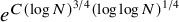
Theorem 1.1. There is a blue-red colouring of  $[N]$ with no blue 3-term progression and no red progression of length $e^{C(\log N)^{3/4}(\log \log N)^{1/4}}$. Consequently, we have the bound
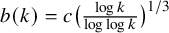
  $w(3,k) \geqslant k^{b(k)}$, where $b(k) = c \big ( \frac {\log k}{\log \log k} \big )^{1/3}$.
Update, June 2022: Nine months after the arxiv version of this paper was made public, Zachary Hunter [Reference Hunter14] was able to simplify parts of the argument and at the same time improve the lower bound to  $w(3,k) \geqslant k^{b'(k)}$, where $b'(k) = c \frac {\log k}{\log \log k}$.
2 Overview and structure the paper
2.1 Discussion and overview
I first heard the question of whether or not  $w(3,k) = O(k^2)$ from Ron Graham in around 2004. My initial reaction was that surely this must be false, for the following reason: take a large subset of $[N]$ free of 3-term progressions, and colour it blue. Then the complement of this set probably does not have overly long red progressions. However, by considering the known examples of large sets free of 3-term progressions, one swiftly becomes less optimistic about this strategy.
Example 1. If we take the blue points to be the folklore example  $\{ \sum _i a_i 3^i : a_i \in \{0,1\}\} \cap [N]$, then the set of red points contains a progression of linear length, namely $\{ n \equiv 2 (\operatorname {mod}\, 3)\}$.
Example 2. If we take the blue points to be the Salem-Spencer set [Reference Salem and Spencer18] or the Behrend set [Reference Behrend3], then one runs into similar issues. Both sets consists of points  $a_1 + a_2 (2d-1) + \dots + a_n (2d - 1)^n$ with all $a_i \in \{0,1,\dots , d-1\}$, and for such sets the red set will contain progressions such as $\{ n \equiv d (\operatorname {mod}\, 2d-1)\}$. If $N := d(2d - 1)^n$, so that the set is contained in $[N]$, the length of such a red progression is $\sim N/d$. In the Behrend case, one takes $d \sim \sqrt {\log N}$, so this is very long.
Example 3. One runs into an apparently different kind of obstacle (although it is closely related) when considering the variant of Behrend’s construction due to Julia Wolf and myself [Reference Green and Wolf11]. (The bound in [Reference Green and Wolf11] was previously obtained by Elkin [Reference Elkin7], but the method of construction in [Reference Green and Wolf11] was different.) Roughly speaking, this construction proceeds as follows. Pick a dimension D, and consider the torus  $\mathbf {T}^D = \mathbf {R}^D/\mathbf {Z}^D$. In this torus, consider a thin annulus, the projection $\pi (A)$ of the set $A = \{ x \in \mathbf {R}^D : \frac {1}{4} - N^{-4/D} \leqslant \Vert x \Vert _2 \leqslant \frac {1}{4}\}$ under the natural map. Pick a rotation $\theta \in \mathbf {T}^D$ at random, and define the blue points to be $\{ n \in [N] : \theta n \in \pi (A)\}$. By simple geometry, one can show that the only 3-term progressions in A are those with very small common difference v, $\Vert v \Vert _2 \ll N^{-4/D}$. This property transfers to $\pi (A)$, essentially because by choosing $\frac {1}{4}$ as the radius of the annulus, one eliminates ‘wraparound effects’, which could have generated new progressions under the projection $\pi $. Due to the choice of parameters, it turns out that with very high probability, there are no blue 3-term progressions at all.
Let us now consider red progressions. Suppose that  $\theta = (\theta _1,\dots , \theta _D)$, and think of D as fixed, with N large. By Dirichlet’s theorem, there is some $d \leqslant \sqrt {N}$ such that $\Vert \theta _1 d \Vert \leqslant 1/\sqrt {N}$, where $\Vert \cdot \Vert _{\mathbf {T}}$ denotes the distance to the nearest integer. Since $\theta $ is chosen randomly, the sequence $(\theta n)_{n = 1}^{\infty }$ will be highly equidistributed, and one certainly expects to find an $n_0 = O_D(1)$ such that $\theta n_0 \approx (\frac {1}{2},\dots , \frac {1}{2})$. If one then considers the progression $P = \{ n_0 + nd : n \leqslant \sqrt {N}/10\}$ (say), one sees that $P \subset [N]$ and $\Vert \theta _1 (n_0 + nd) - \frac {1}{2} \Vert _{\mathbf {T}} < \frac {1}{4}$ for all $n \leqslant \sqrt {N}/10$. That is, all points of P avoid the annulus $\pi (A)$ (and in fact the whole ball of radius $\frac {1}{4}$) since their first coordinates are confined to a narrow interval about $\frac {1}{2}$. Therefore, P is coloured entirely red.
This last example does rather better than Examples 1 and 2, and it is the point of departure for the construction in this paper. Note that, in Example 3, the progression P of length  $\gg \sqrt {N}$ that we found is not likely to be the only one. One could instead apply Dirichlet’s theorem to any of the other coordinates $\theta _2,\dots , \theta _D$. Moreover, one could also apply it to $\theta _1 + \theta _2$, noting that points $x \in \pi (A)$ satisfy $\Vert x_1 + x_2 \Vert _{\mathbf {T}} \leqslant \frac {\sqrt {2}}{4}$ and so avoid a narrow ‘strip’ $\Vert x_1 + x_2 - \frac {1}{2} \Vert _{\mathbf {T}} \leqslant \frac {1}{2} - \frac {\sqrt {2}}{4}$, or to $\theta _1 + \theta _2 + \theta _3$, noting that points $x \in \pi (A)$ satisfy $\Vert x_1 + x_2 + x_3 \Vert _{\mathbf {T}} \leqslant \frac {\sqrt {3}}{4}$ and so avoid a narrow strip $\Vert x_1 + x_2 + x_3 - \frac {1}{2} \Vert _{\mathbf {T}} \leqslant \frac {1}{2} - \frac {\sqrt {3}}{4}$. However, this no longer applies to $\theta _1 + \theta _2 + \theta _3 + \theta _4$, since the relevant strip has zero width.
This discussion suggests the following key idea: instead of one annulus  $\pi (A)$, we could try taking several, in such a way that every strip like the ones just discussed intersects at least one of these annuli. This then blocks all the ‘obvious’ ways of making red progressions of length $\sim \sqrt {N}$. Of course, one then runs the risk of introducing blue 3-term progressions. However, by shrinking the radii of the annuli to some $\rho \lll 1$, a suitable construction may be achieved by picking the annuli to be random translates of a fixed one.
At this point we have an annulus  $A = \{ x \in \mathbf {R}^D : \rho - N^{-4/D} \leqslant \Vert x \Vert _2 \leqslant \rho \}$ together with a union of translates $S := \bigcup _{i=1}^M (x_i + \pi (A)) \subset \mathbf {T}^D$. Pick $\theta \in \mathbf {T}^D$ at random, and colour those $n \leqslant N$ for which $\theta n \in S$ blue. As we have stated, it is possible to show that (with a suitable choice of $\rho $, and for random translates $x_1,\dots , x_M$ with M chosen correctly) there are likely to be no blue 3-term progressions. Moreover, the obvious examples of red progressions of length $\sim \sqrt {N}$ coming from Dirichlet’s theorem are blocked.
Now one may also apply Dirichlet’s theorem to pairs of frequencies, for instance producing  $d \leqslant N^{2/3}$ such that $\Vert \theta _1 d\Vert _{\mathbf {T}}, \Vert \theta _2 d \Vert _{\mathbf {T}} \leqslant N^{-1/3}$ and thereby potentially creating red progressions of length $\sim N^{1/3}$ unless they too are blocked by the union of annuli. To obstruct these, one needs to consider ‘strips’ of codimension $2$, for instance given by conditions such as $x_1, x_2 \approx \frac {1}{2}$. Similarly, to avoid progressions of length $\sim N^{1/4}$, one must ensure that strips of codimension $3$ are blocked, and so on.
Using these ideas, one can produce, for arbitrarily large values of r, a red–blue colouring of  $[N]$ with no blue 3-term progression and no obvious way to make a red progression of length $N^{1/r}$. Of course, this is by no means a proof that there are no such red progressions!
Let us now discuss a further difficulty that arises when one tries to show that there no long red progressions. Consider the most basic progression  $P = \{ 1, 2,\dots , X\}$, $X = N^{1/r}$, together with the task of showing it has at least one blue point. Suppose that $x_1$ (the centre of the first annulus in S) is equal to $0 \in \mathbf {T}^D$. Then, since P is ‘centred’ on $0$, it is natural to try to show that $\{ \theta , 2\theta ,\dots , X \theta \}$ intersects the annulus $\pi (A)$ with centre $x_1 = 0$, or in other words to show that there is $n \leqslant X$ such that
 $$ \begin{align} (\rho - N^{-4/D})^2 < \Vert n \theta_1 \Vert_{\mathbf{T}}^2 + \dots + \Vert n \theta_D \Vert_{\mathbf{T}}^2 < \rho^2.\end{align} $$
The general flavour of this problem is to show that a certain ‘quadratic form’ takes at least one value in a rather small interval. However, what we have is not a bona fide quadratic form. To make it look like one, we apply standard geometry of numbers techniques to put a multidimensional structure on the Bohr set of n such that  $\Vert n \theta _1 \Vert _{\mathbf {T}},\dots , \Vert n \theta _D \Vert _{\mathbf {T}} \leqslant \frac {1}{10}$ (say). This gives, inside the set of such n, a multidimensional progression $\{ \ell _1 n_1 + \dots + \ell _{D+1} n_{D+1} : 0 \leqslant \ell _i < L_i\}$ for certain $n_i$ and certain lengths $L_i$. The size $L_1 \cdots L_{D+1}$ of this progression is comparable to X.
In this ‘basis’, the task in equation (2.1) then becomes to show that there are  $\ell _1,\dots , \ell _{D+1}$, $0 \leqslant \ell _i < L_i$, such that
 $$ \begin{align} (\rho - N^{-4/D})^2 < q(\ell_1,\dots, \ell_{D+1}) < \rho^2, \end{align} $$
where q is a certain quadratic form depending on  $n_1,\dots , n_{D+1}$ and $\theta $. A representative case (but not the only one we need to consider) would be $L_1 \approx \dots \approx L_{D+1} \approx L = X^{1/(D+1)}$, with the coefficients of q having size $\sim L^{-2}$ so that q is bounded in size by $O(1)$. Note that $N^{-4/D} \approx L^{-4r}$. Thus we have a problem of roughly the following type: given a quadratic form $q : \mathbf {Z}^{D+1} \rightarrow \mathbf {R}$ with coefficients of size $\sim L^{-2}$, show that on the box $[L]^{D+1}$, it takes at least one value on some given interval of length $L^{-4r}$.
Without further information, this is unfortunately a hopeless situation because of the possibility that, for instance, the coefficients of q lie in  $\frac {1}{Q} \mathbf {Z}$ for some $Q> L^2$. In this case, the values taken by q are $\frac {1}{Q}$-separated and hence, for moderate values of Q, not likely to lie in any particular interval of length $L^{-4r}$.
A small amount of hope is offered by the fact that q is not a fixed quadratic form – it depends on the random choice of  $\theta $. However, the way in which random $\theta $ correspond to quadratic forms is not at all easy to analyse, and moreover we also need to consider similar problems for $2\theta , 3 \theta ,\dots $ corresponding to potential red progressions with common difference $d = 2,3,\dots $.
Our way around this issue, and the second key idea in the paper, is to introduce a large amount of extra randomness elsewhere, in the definition of the annuli. Instead of the standard  $\ell ^2$-norm $\Vert x \Vert _2$, we consider instead a perturbation $\Vert (I + E) x \Vert _2$, where E is a random $D \times D$ matrix with small entries so that $I+E$ is invertible with operator norm close to $1$. Such ellipsoidal annuli are just as good as spherical ones for the purposes of our construction. The choice of E comes with a massive $D(D+1)/2$ degrees of freedom (not $D^2$, because Es that differ by an orthogonal matrix give the same norm). The quadratic form q then becomes a random quadratic form $q_E$.
With considerable effort, the distribution of  $q_E$, E random, can be shown to be somewhat related (for typical $\theta $) to the distribution of a truly random quadratic form $q_a(\ell _1,\dots , \ell _{D+1}) = \sum _{i\leqslant j} a_{ij} \ell _i \ell _j$, with the coefficients chosen uniformly from $|a_{ij}| \leqslant L^{-2}$. One is then left with the task of showing that a uniformly random quadratic form $q_a$ takes values in a very short interval of length $L^{-4r}$. Moreover, this is required with a very strong bound on the exceptional probability, suitable for taking a union bound over the $\sim N^{1 - 1/r}$ possible choices of the common difference d.
A natural tool for studying gaps in the values of quadratic forms is the Hardy-Littlewood circle method, and indeed it turns out that a suitable application of the Davenport-Heilbronn variant of the method can be applied to give what we require. The application is not direct and additionally requires a novel amplification argument using lines in the projective plane over a suitable  $\mathbf {F}_p$ to get the strong bound on the exceptional probability that we need.
The above sketch omitted at least one significant detail, namely how to handle ‘uncentred’ progressions P starting at points other than  $0$. For these, one must use the particular choice of the centres $x_i$. One can show that P enters inside at least one of the balls $x_i + \pi (B_{\rho /10}(0))$, and starting from here one can proceed much as in the centred case.
2.2 Structure of the paper
With that sketch of the construction complete, let us briefly describe the structure of the paper. As the above discussion suggests, it is natural to introduce a parameter r and consider the following equivalent form of Theorem 1.1.
Theorem 2.1. Let r be an integer, and suppose that  $N> e^{Cr^4 \log r}$. Then there is a red/blue colouring of $[N]$ with no blue 3-term progression and no red progression of length $N^{1/r}$.
Taking  $r = c \big ( \frac {\log N}{\log \log N} \big )^{1/4}$ for suitable c, we recover Theorem 1.1. While Theorems 1.1 and 2.1 are equivalent, it is much easier to think about Theorem 2.1 and its proof by imagining that r is fixed and N is a very large compared to r. We will, of course, keep track of just how large N needs to be as we go along, but this is somewhat secondary to understanding the key concepts of the argument. For the rest of the paper, r will denote the parameter appearing in Theorem 2.1, and we will always assume (as we clearly may) that it is sufficiently large.
In Section 3, we summarise some key notation and conventions in force for the rest of the paper. In Section 4, we turn to the details of our construction, in particular constructing the translates  $x_1,\dots , x_M$ of our annuli, and introducing the notion of a random ellipsoidal annulus properly. In Section 5, we describe the red/blue colouring itself and divide the task of showing that there are no blue 3-term progressions or red $N^{1/r}$-term progressions into three parts (the blue progressions, and what we call steps 1 and 2 for the red progressions). In Section 6, we handle the blue 3-term progressions. Section 7 is then devoted to a technical ‘diophantine’ condition on $\theta \in \mathbf {T}^D$ that will be in force for the rest of the paper. In Section 8, we handle step 1 of the treatment of red progressions.
At this point we are only one third of the way through the paper. The remaining discussion is devoted to the treatment of step 2 for the red progressions, which involves the geometry of numbers and gaps in random quadratic forms material outlined above. We devote Section 9 to a more detailed technical overview of the argument that reduces it to three key propositions. The proofs of these propositions are then handled in Parts IV and V of the paper. Part IV contains, roughly speaking, the relevant geometry of numbers arguments, whilst Part V contains the arguments pertaining to gaps in quadratic forms. These parts may be read independently of one another and of the rest of the paper.
2.3 Further comments
The discussion around the application of Dirichlet’s theorem above suggests that there are certain ‘phase changes’ in the problem as one goes from ruling out red progressions of length  $\sim N^{1/2}$ to ruling out progressions of length $\sim N^{1/3}$, and so on. Indeed, this is why we formulate our main result in the equivalent form of Theorem 2.1. I consider it quite plausible that such phase changes are not merely an artefact of our argument but rather of the problem as a whole, and the apparently strong numerical evidence for quadratic behaviour of $w(3,k)$ reflects the fact that in the regime $k \leqslant 40$, one is only seeing the first phase in which it is more efficient to take just one large annulus as in the construction of Julia Wolf and myself, at the expense of having to allow strips of codimension 1 that admit red progressions of length $\sim N^{1/2}$. It would be interesting to see whether the ideas of this paper could be used to produce, computationally, an example with $w(3,k) \sim k^3$.
I have worked quite hard to try to optimise the exponent in Theorem 1.1, and it seems to represent the limit of the method for multiple different reasons, as discussed in a little more detail in Section 3 below. These limitations seem to be a mix of fundamental ones and artefacts of our analysis. I would expect that the true value of  $w(3,k)$ lies somewhere in between the bound of Theorem 1.1 and something like $k^{c\log k}$, which is what a Behrend construction of the blue points would give if only the complement of such a set ‘behaved randomly’. Ron Graham [Reference Graham10] established a lower bound of this type for a restricted version of the problem in which one only forbids red progressions with common difference $1$.
$1$.
Finally, we remark that [Reference Fox and Pohoata9] is an earlier example in which random unions of structured objects are used to understand a problem related to arithmetic progressions.
3 Notation and conventions
3.1 Fourier transforms
We use the standard notation  $e(t) := e^{2\pi i t}$ for $t \in \mathbf {R}$.
We will take Fourier transforms of functions on  $\mathbf {R}^k, \mathbf {Z}^k, \mathbf {T}^k$ for various integers k. We will use the same hat symbol for all of these and define them as follows:
• If $f : \mathbf {R}^k \rightarrow \mathbf {C}$, $\hat {f}(\gamma ) = \int _{\mathbf {R}^k} f(x) e(-\langle \gamma , x\rangle ) dx$ for $\gamma \in \mathbf {R}^k$;
• If
$f : \mathbf {Z}^k \rightarrow \mathbf {C}$, $\hat {f}(\theta ) = \sum _{n \in \mathbf {Z}^k} f(n) e(-n \cdot \theta )$ for $\theta \in \mathbf {T}^k$;• If
$f : \mathbf {T}^k \rightarrow \mathbf {C}$, $\hat {f}(\xi ) = \int _{\mathbf {T}^k} f(x) e(-\xi \cdot x) dx$ for $\xi \in \mathbf {Z}^k$.


The notation  $\langle x, y\rangle $ for $\sum _i x_i y_i$ in $\mathbf {R}^k$, but $x \cdot y$ in $\mathbf {Z}^k$ and $\mathbf {T}^k$, is merely cultural and is supposed to reflect the fact that our arguments in the former space will be somewhat geometric in flavour.
We will only be using the Fourier transform on smooth, rapidly decaying functions where convergence issues are no problem. Note in particular that the normalisation of the Fourier transform on  $\mathbf {R}^k$ (with the phase multiplied by $2\pi $) is just one of the standard options, but a convenient one in this paper. With this normalisation, Fourier inversion states that $f(x) = \int _{\mathbf {R}^k} \hat {f}(\gamma ) e(\langle \gamma , x\rangle ) d\gamma $.
3.2 Convention on absolute constants
It would not be hard to write in explicit constants throughout the paper. They would get quite large, but not ridiculously so. However, we believe it makes the presentation neater, and the dependencies between parameters easier to understand, if we leave the larger ones unspecified and adopt the following convention:
•
$C_1$ is a sufficiently large absolute constant;•
$C_2$ is an even larger absolute constant, how large it needs to be depending on the choice of $C_1$;•
$C_3$ is a still larger constant, large enough in terms of $C_1, C_2$.


To clarify, no matter which  $C_1$ we choose (provided it is sufficiently big), there is an appropriate choice of $C_2$, and in fact all sufficiently large $C_2$ work. No matter which $C_2$ we choose, all sufficiently large $C_3$ work. There are many constraints on how large $C_1$ needs to be throughout the paper, and it must be chosen to satisfy all of them, and similarly for $C_2, C_3$.
3.3 Key parameters
The most important global parameters in the paper are the following:
• N: the interval
$[N]$ is the setting for Theorem 2.1.• r: a positive integer, always assumed to be sufficiently large.
$N^{1/r}$ is the length of red progressions we are trying to forbid.• D: a positive integer dimension. The torus
$\mathbf {T}^D = \mathbf {R}^D/\mathbf {Z}^D$ will play a key role in the paper.


Throughout the paper, we will assume that
 $$ \begin{align} r \ \mbox{sufficiently large}, \qquad D = C_3 r^2, \qquad N \geqslant D^{C_2 D^2}.\end{align} $$
Several lemmas and propositions do not require such strong assumptions. However, two quite different results in the paper (Proposition 4.1 and the application of Proposition 9.3 during the proof of Proposition 5.4 in Section 9) require a condition of the form  $D \gg r^2$. The condition $N> D^{C_2 D^2}$ comes up in the proof of Proposition 5.4, in fact in no fewer than three different ways in the last displayed equation of Section 9. For these reasons, it seems as if our current mode of argument cannot possibly yield anything stronger than Theorem 2.1.
A number of other parameters and other nomenclature feature in several sections of the paper:
• X: shorthand for
$N^{1/r}$.•
$\theta $: an element of $\mathbf {T}^D$, chosen uniformly at random, and later in the paper always taken to lie in the set $\Theta $ of diophantine elements (Section 7).•
$\rho $: a small radius (of annuli in $\mathbf {T}^D$), from Section 5 onwards fixed to be $D^{-4}$.•
$\mathbf {e}$: a uniform random element of $[-\frac {1}{D^4} , \frac {1}{D^4} ]^{D(D+1)/2}$ (used to define random ellipsoids). Usually we will see $\sigma (\mathbf {e})$, which is a symmetric matrix formed from $\mathbf {e}$ in an obvious way (see Section 4 for the definition).• d: invariably the common difference of a progression, with
$d \leqslant N/X$.


The letter Q is reserved for a ‘complexity’ parameter (bounding the allowed size of coefficients, or of matrix entries) in various different contexts.
3.4 Notation $[N]$ always denotes $\{1,\dots , N\}$.
If  $x \in \mathbf {T}$, then we write $\Vert x \Vert _{\mathbf {T}}$ for the distance from x to the nearest integer. If $x = (x_1,\dots , x_D) \in \mathbf {T}^D$, then we write $\Vert x \Vert _{\mathbf {T}^D} = \max _i \Vert x_i \Vert _{\mathbf {T}}$.
We identify the dual  $\hat {\mathbf {T}}^D$ with $\mathbf {Z}^D$ via the map $\xi \mapsto (x \mapsto e(\xi \cdot x))$, where $\xi \cdot x = \xi _1 x_1 + \cdots + \xi _D x_D$. In this setting, we always write $|\xi | := \max _i |\xi _i|$ instead of the more cumbersome $\Vert \xi \Vert _{\infty }$.
Apart from occasional instances where it denotes  $3.141592\dots $, $\pi $ is the natural projection homomorphism $\pi : \mathbf {R}^D \rightarrow \mathbf {T}^D$. Clearly $\pi $ is not invertible, but nonetheless we abuse notation by writing $\pi ^{-1}(x)$ for the unique element $y \in (-\frac {1}{2}, \frac {1}{2}]^D$ with $\pi (y) = x$.
If R is a  $D \times D$ matrix over $\mathbf {R}$, then we write $\Vert R \Vert $ for the $\ell ^2$-to- $\ell ^2$ operator norm, that is to say $\Vert Rx \Vert _{2} \leqslant \Vert R \Vert \Vert x \Vert _2$, and $\Vert R \Vert $ is the smallest constant with this property. Equivalently, $\Vert R \Vert $ is the largest singular value of R.
Part II A red/blue colouring of  $ [\boldsymbol{N}]$
4 Random ellipsoidal annuli
In this section, we prepare the ground for describing our red/blue colouring of  $[N]$, which we will give in Section 5. In the next section, we describe our basic construction by specifying the points in $[N]$ to be coloured blue. The torus $\mathbf {T}^D$ (and Euclidean space $\mathbf {R}^D$) play a fundamental role in our construction, where $D = C_3 r^2$.
4.1 A well-distributed set of centres
As outlined in Section 2, an important part of our construction is the selection (randomly) of a certain set  $x_1,\dots , x_M$ of points in $\mathbf {T}^D$. Later, we will fix $\rho := D^{-4}$, but the following proposition does not make any assumption on $\rho $ beyond that $\rho < D^{-1}$.
Proposition 4.1. Suppose that  $D = C_3 r^2$ and $\rho < \frac {1}{D}$. There are $x_1,\dots , x_M \in \mathbf {T}^D$ such that the following hold:
1. Whenever
$i_1, i_2, i_3$ are not all the same, $\Vert x_{i_1} - 2 x_{i_2} + x_{i_3} \Vert _{\mathbf {T}^D} \geqslant 10 \rho $.2. Whenever
$V \leqslant \mathbf {Q}^D$ is a subspace of dimension at most $4r$ and $x \in \mathbf {T}^D$, there is some j such that $\Vert \xi \cdot (x_j - x) \Vert _{\mathbf {T}} \leqslant \frac {1}{100}$ for all $\xi \in V \cap \mathbf {Z}^D$ with $|\xi | \leqslant \rho ^{-3}$.


Remark. With reference to the outline in Section 2, condition (2) here is saying that any ‘slice’ of codimension at most  $4r$ contains one of the $x_i$; this is what obstructs a simple construction of red progressions of length $N^{1/r}$ using Dirichlet’s theorem. Item (1) will allow us to guarantee that by taking a union of translates of annuli, rather than just one, we do not introduce new blue 3-term progressions.
Proof. Set  $M = \lceil \rho ^{-D/4}\rceil $, and pick $x_1,\dots , x_M \in \mathbf {T}^D$ independently and uniformly at random. For any triple $(i_1, i_2, i_3)$ with not all the indices the same, $x_{i_1} - 2x_{i_2} + x_{i_3}$ is uniformly distributed on $\mathbf {T}^D$. Therefore, $\mathbb {P} ( \Vert x_{i_1} - 2 x_{i_2} + x_{i_3} \Vert _{\mathbf {T}^D} \leqslant 10 \rho ) \leqslant (20 \rho )^{D}$. Summing over all $< M^3$ choices of indices gives an upper bound of $M^3 (20 \rho )^D < \frac {1}{4}$ on the probability that (1) fails (since D is sufficiently large).
For (2), we may assume that V is spanned (over  $\mathbf {Q}$) by vectors $\xi \in \mathbf {Z}^D$ with $|\xi | \leqslant \rho ^{-3}$ (otherwise, pass from V to the subspace of V spanned by such vectors). There are at most $4r (3 \rho ^{-3})^{4r D} < \rho ^{-14rD}$ such V (choose the dimension $m < 4r$, and then m basis elements with $\xi \in \mathbf {Z}^D$ and $|\xi | \leqslant \rho ^{-3}$).
Fix such a V. By Lemma 1.2,  $V \cap \mathbf {Z}^D$ is a free $\mathbf {Z}$-module generated by some $\xi _1,\dots , \xi _m$, $m \leqslant 4r$, and with every element $\xi \in V \cap \mathbf {Z}^D$ with $|\xi | \leqslant \rho ^{-3}$ being $\xi = n_1 \xi _1+ \cdots + n_m \xi _m$ with $|n_i| \leqslant m! (2\rho ^{-3})^m \leqslant \frac {1}{400r}\rho ^{-14 r}$. Thus, to satisfy our requirement, we need only show that for any $x \in \mathbf {T}^D$ there is $x_j$ such that
 $$ \begin{align} \Vert \xi_i \cdot (x_j - x) \Vert_{\mathbf{T}} \leqslant \rho^{14r} \; \mbox{for} \ i = 1,\dots, m, \end{align} $$
since then
 $$\begin{align*}\Vert \xi \cdot (x_j - x) \Vert_{\mathbf{T}} \leqslant \rho^{14r}\sum_{i = 1}^m |n_i| < \frac{1}{100}.\end{align*}$$
 Divide  $\mathbf {T}^m$ into $\rho ^{- 14 rm} \leqslant \rho ^{-56r^2}$ boxes of side length $\rho ^{14 r}$; it is enough to show that each such box B contains at least one point $(\xi _1 \cdot x_j, \cdots \xi _m \cdot x_j)$. The following fact will also be needed later, so we state it as a separate lemma.
Lemma 4.2. Let  $\xi _1,\dots , \xi _m \in \mathbf {Z}^D$ be linearly independent. Then as x ranges uniformly over $\mathbf {T}^D$, $(\xi _1 \cdot x, \cdots , \xi _m \cdot x)$ ranges uniformly over $\mathbf {T}^m$.
Proof. Let  $f(t) = e(\gamma \cdot t)$ be a nontrivial character on $\mathbf {T}^{m}$. Then
 $$\begin{align*}\int_{\mathbf{T}^D} f(\xi_1 \cdot x, \dots, \xi_m \cdot x) dx = \int_{\mathbf{T}^D} e( (\gamma_1 \xi_1 + \cdots + \gamma_{m} \xi_{m}) \cdot x)dx = 0 = \int_{\mathbf{T}^m} f,\end{align*}$$
since  $\gamma _1 \xi _1 + \dots + \gamma _m \xi _m \neq 0$. Since the characters are dense in $L^1(\mathbf {T}^m)$, the result follows.
Returning to the proof of Proposition 4.1, Lemma 4.2 implies that for each fixed j,
 $$\begin{align*}\mathbb{P}( (\xi_1 \cdot x_j, \dots , \xi_m \cdot x_j) \notin B ) = 1 - \rho^{14rm}.\end{align*}$$
By independence,
 $$ \begin{align*} \mathbb{P} ( (\xi_1 \cdot x_j, \dots , \xi_m \cdot x_j) \notin & \; B \; \mbox{for } \ j = 1,\dots, M ) \\ & = (1 - \rho^{14rm})^M \leqslant e^{-\rho^{14rm} M} \leqslant e^{-\rho^{-D/8}}. \end{align*} $$
 Here we critically use that  $D = C_3 r^2$; $C_3 \geqslant 448$ is sufficient here, but it will need to be larger than this in later arguments. Summing over the boxes B, we see that the probability of even one empty box is $\leqslant \rho ^{-56 r^2} e^{-\rho ^{-D/8}}$. This is the probability that equation (4.1) does not hold for this particular V. Summing over the $\leqslant \rho ^{-14 D r}$ choices for V, the probability that equation (4.1) fails to hold for some V is
 $$\begin{align*}\leqslant \rho^{-16 D r} e^{-\rho^{-D/8}}.\end{align*}$$
For D large, this will be  $< \frac {1}{4}$ as well, uniformly in $\rho $. (To see this, write $X = 1/\rho> D$; then this function is bounded by $X^{D^2} e^{-X^{D/8}}$, which is absolutely tiny on the range $X> D$.)
It follows that, with probability  $> \frac {1}{2}$ in the choice of $x_1,\dots , x_M$, both (1) and (2) hold.
4.2 Random ellipsoidal annuli
Our construction is based on annuli centred on the points  $x_1,\dots , x_M$ just constructed. As outlined in Section 2, so as to introduce a source of randomness into the problem, we consider, rather than just spherical annuli, random ellipsoidal annuli.
To specify the ellipsoids, here and throughout the paper identify  $\mathbf {R}^{D(D+1)/2}$ with the space of all tuples $x = (x_{ij})_{1 \leqslant i \leqslant j \leqslant D}$. Let $\mathbf {e}$ be a random tuple uniformly sampled from $[-\frac {1}{D^4} , \frac {1}{D^4} ]^{D(D+1)/2} \subset \mathbf {R}^{D(D+1)/2}$.
To any tuple  $x \in \mathbf {R}^{D(D+1)/2}$, we associate a symmetric matrix $\sigma (x) \in \operatorname {Sym}_D(\mathbf {R})$ (the space of $D \times D$ symmetric matrices over $\mathbf {R}$) as follows: $(\sigma (x))_{ii} = x_{ii}$, $(\sigma (x))_{ij} = \frac {1}{2}x_{ij}$ for $i < j$, and $(\sigma (x))_{ij} = \frac {1}{2}x_{ji}$ for $i> j$.
The ellipsoidal annuli we consider will then be of the form  $\pi (A_{\mathbf {e}})$, where $\pi : \mathbf {R}^D \rightarrow \mathbf {T}^D$ is the natural projection and
 $$ \begin{align} A_{\mathbf{e}} := \{ x \in \mathbf{R}^D : \rho - N^{-4/D} < \Vert (I + \sigma(\mathbf{e})) x \Vert_2 < \rho\}.\end{align} $$
It is convenient to fix, for the rest of the paper,
 $$ \begin{align} \rho := D^{-4}; \end{align} $$
the choice is somewhat arbitrary, and any sufficiently large power of  $1/D$ would lead to essentially the same bounds in our final result. With this choice, the parameter M in Proposition 4.1 (that is, the number of points $x_1,\dots , x_M$) is $D^D$.
Now  $\Vert \sigma (e) \Vert \leqslant D \Vert e \Vert _{\infty } \leqslant \frac {1}{2}$, where $\Vert \cdot \Vert $ denotes the $\ell ^2$-to- $\ell ^2$ operator norm on matrices, and therefore
 $$ \begin{align} \frac{1}{2} \leqslant \Vert I + \sigma(\mathbf{e}) \Vert \leqslant \frac{3}{2}. \end{align} $$
Remark. Taking  $\sigma (\mathbf {e})$ to be symmetric is natural in view of the polar decomposition of real matrices. Premultiplying $\sigma (\mathbf {e})$ by an orthogonal matrix makes no difference to $\Vert (I + \sigma (\mathbf {e}) ) x\Vert _2$.
5 The colouring. Outline proof of the main theorem
We are now in a position to describe our red/blue colouring of  $[N]$. Once again let $r, D$ be integers with r sufficiently large and $D = C_3 r^2$. Set $\rho := D^{-4}$, and let $x_1,\dots , x_M \in \mathbf {T}^D$ be points as constructed in Proposition 4.1 for this value of $\rho $. Pick $\mathbf {e} \in [-\frac {1}{D^4} , \frac {1}{D^4} ]^{D(D+1)/2} \subset \mathbf {R}^{D(D+1)/2}$ uniformly at random, and consider the random ellipsoidal annulus
 $$\begin{align*}A_{\mathbf{e}} := \{ x \in \mathbf{R}^D : \rho - N^{-4/D} < \Vert (I + \sigma(\mathbf{e})) x \Vert_2 < \rho\}.\end{align*}$$
 Pick  $\theta \in \mathbf {T}^D$ uniformly at random, let $\pi : \mathbf {R}^D \rightarrow \mathbf {T}^D$ be the natural projection, and define a red/blue colouring by
 $$ \begin{align} \operatorname{Blue}_{\mathbf{e},\theta} := \{ n \in [N] : \theta n \in \bigcup_{j=1}^M (x_j + \pi(A_{\mathbf{e}}) \}, \end{align} $$
 $$ \begin{align} \operatorname{Red}_{\mathbf{e},\theta} := [N] \setminus \operatorname{Blue}_{\mathbf{e},\theta}.\end{align} $$
 Suppose henceforth that  $N> D^{C_2 D^2}$, this being stronger than needed for some results but necessary in the worst case. We claim that with high probability there is no blue progression of length $3$.
$3$.
Proposition 5.1. Suppose that  $N> D^{C_2D^2}$. Then
 $$\begin{align*}\mathbb{P}_{\theta, \mathbf{e}} \big( \operatorname{Blue}_{\theta, \mathbf{e}} \mbox{has no 3-term progression} \big) \geqslant 1 - O(N^{-1}). \end{align*}$$
 In dealing with the progressions in the red points, we introduce a specific set  $\Theta $ of rotations $\theta \in \mathbf {T}^D$ that we wish to consider. We call $\Theta $ the set of diophantine $\theta $: the terminology is not standard, but the word diophantine is used in similar ways in other contexts. The precise definition of $\Theta $ is given in Section 7 below. Roughly, $\theta $ is disqualified from $\Theta $ if the orbit $\{ \theta n : n \leqslant N\}$ exhibits certain pathological behaviours such as being highly concentrated near $0$ or having long subprogressions almost annihilated by a large set of characters on $\mathbf {T}^D$. For our discussion in this section, the important fact about $\Theta $ is that diophantine elements are (highly) generic in the sense that
 $$ \begin{align} \mu_{\mathbf{T}^D} (\Theta) \geqslant 1 - O(N^{-1}). \end{align} $$
This is proven in Section 7, specifically Proposition 7.1, where the definition of  $\Theta $ is given.
Now we claim that, conditioned on the event that  $\theta $ is diophantine, with high probability there is no red progression of length $N^{1/r}$.
Proposition 5.2. Suppose that  $N> D^{C_2D^2}$. Then
 $$\begin{align*}\mathbb{P}_{\mathbf{e}} \big( \operatorname{Red}_{\theta, \mathbf{e}} \ \mbox{has no} \ N^{1/r}\mbox{-term progression} \; | \; \theta \in \Theta \big) \geqslant 1 - O(N^{-1}), \end{align*}$$
where  $\Theta \subset \mathbf {T}^D$ denotes the set of diophantine elements.
The proof of Proposition 5.1 is relatively straightforward and is given in Section 6. The proof of Proposition 5.2 is considerably more involved and occupies the rest of the paper.
Let us now show how Theorem 2.1 follows essentially immediately from Propositions 5.1 and 5.2.
Proof of Theorem 2.1.
(assuming Propositions 5.1 and 5.2) First observe that, with  $D = C_3 r^2$, the conditions required in Propositions 5.1 and 5.2 will be satisfied if $N> e^{C r^4 \log r}$ for a sufficiently large C. Also, in proving Theorem 2.1, we may clearly assume that r is sufficiently large.
First note that by Proposition 5.2 and equation (5.3), we have
 $$\begin{align*}\mathbb{P}_{\theta, \mathbf{e}} \big( \operatorname{Red}_{\theta, \mathbf{e}} \ \mbox{has no} \ N^{1/r}\mbox{-term progression} \big) \geqslant 1 - O(N^{-1}). \end{align*}$$
This and Proposition 5.1 imply that there is some choice of  $\theta , \mathbf {e}$ (in fact, a random choice works with very high probability) for which simultaneously $\operatorname {Blue}_{\theta , \mathbf {e}}$ has no 3-term progression and $\operatorname {Red}_{\theta , \mathbf {e}}$ has no $N^{1/r}$-term progression. This completes the proof of Theorem 2.1.
Let us consider the task of proving Proposition 5.2 in a little more detail. Let
 $$ \begin{align} X := N^{1/r}, \end{align} $$
a notational convention we will retain throughout the paper.
It suffices to show that if  $N> D^{C_2D^2}$ and $\theta \in \Theta $ is diophantine, then for each fixed progression $P = \{n_0 + dn : n \leqslant X \} \subset [N]$ of length X,
 $$ \begin{align} \mathbb{P}_{\mathbf{e}} (P \cap \operatorname{Blue}_{\theta, \mathbf{e}} = \emptyset) \leqslant N^{-3}. \end{align} $$
Indeed, there are fewer than  $N^2$ choices of $n_0$ and d, the start point and common difference of P, so Proposition 5.2 follows from equation (5.5) by the union bound.
The task, then, is to show that (with very high probability)  $\theta P \subset \mathbf {T}^D$ intersects one of the annuli $x_j + \pi (A_{\mathbf {e}})$. To achieve this, we proceed in two distinct stages. Denoting by $P_{\operatorname {init}} = \{ n_0 + dn : n \leqslant X/2\}$ the first half of P, we show that $\theta P_{\operatorname {init}}$ at some point enters the interior of some ball $x_j + \pi (B_{\rho /10}(0))$, where $B_{\varepsilon }(0) \subset \mathbf {R}^D$ is the Euclidean ball of radius $\varepsilon $, and as usual $\pi : \mathbf {R}^D \rightarrow \mathbf {T}^D$ is projection. This we call the first step.
Proposition 5.3 (First step)
Suppose that  $N> D^{C_2 D^2}$. Let $\theta \in \Theta $ be diophantine. Let $d \leqslant N/X$, and consider a progression $P_{\operatorname {init}} = \{n_0 + dn : n \leqslant X/2\}$. Then $\theta P_{\operatorname {init}}$ intersects $x_j + \pi (B_{\rho /10}(0))$ for some $j \in \{1,\dots , M\}$.
Once we have a point of  $\theta P_{\operatorname {init}}$ in $x_j + \pi (B_{\rho /10}(0))$, we use the remaining half of P to intersect the annulus $x_j + \pi (A_{\mathbf {e}})$. This we call the second step.
Proposition 5.4 (Second step)
Suppose that  $N \geqslant D^{C_2D^2}$. Let $d \leqslant N/X$. Suppose that $\theta \in \Theta $ is diophantine, and consider a progression $\dot {P} = \{ dn : n \leqslant X/2\}$. Then
 $$\begin{align*}\mathbb{P}_{\mathbf{e}} (\mbox{there is} \ y \in \pi(B_{\rho/10}(0))\ \mbox{such that} \ (y + \theta \dot{P}) \cap \pi(A_{\mathbf{e}}) = \emptyset) \leqslant N^{-3}.\end{align*}$$
 Together, Propositions 5.3 and 5.4 imply equation (5.5) and hence, as explained above, Proposition 5.2. Indeed, Proposition 5.3 implies that there is some  $n_0 + n_1 d \in P_{\operatorname {init}}$ (that is, some $n_1 \leqslant X/2$ such that $\theta (n_0 + n_1 d) \in x_j + \pi (B_{\rho /10}(0))$, for some $j \in \{1,\dots , M\}$). Now apply Proposition 5.4, taking $y = \theta (n_0 + n_1d) - x_j$. With probability $1 - O(N^{-3})$ in the choice of $\mathbf {e}$, this provides some $n_2 d \in \dot {P}$ (that is, $n_2 \leqslant X/2$) such that $y + \theta n_2 d \in \pi (A_{\mathbf {e}})$.
If  $n_1, n_2$ can both be found (which happens with probability $1 - O(N^{-3})$ in the choice of $\mathbf {e}$), then
 $$\begin{align*}\theta(n_0 + (n_1 + n_2) d) - x_j \in \pi(A_{\mathbf{e}}), \end{align*}$$
which means  $n_0 + (n_1 + n_2)d$ is coloured blue. This establishes equation (5.5).
The remaining tasks in the paper are therefore as follows.
• Establish Proposition 5.1 (blue 3-term progressions). This is relatively straightforward and is covered in Section 6.
• Give the full definition of
$\Theta $ and the set of diophantine $\theta $, and prove equation (5.3). This is carried out in Section 7.• Prove Proposition 5.3, the ‘first step’ for the red progressions. This is carried out in Section 8.
• Prove Proposition 5.4, the ‘second step’ for the red progressions.


The first three tasks, as well as an outline of the fourth, are carried out in Part III of the paper (Sections 6, 7, 8 and 9, respectively).
The fourth task (proving Proposition 5.4) is very involved. We give a technical outline in Section 9, which reduces it to the task of proving three further propositions: Propositions 9.1, 9.2 and 9.3. These propositions are established in Parts IV and V of the paper.
Part III Monochromatic progressions
6 No blue 3-term progressions
In this section, we establish Proposition 5.1. Let us recall the statement.
Proposition 5.1. Suppose that  $N> D^{C_2D^2}$. Then
 $$\begin{align*}\mathbb{P}_{\theta, \mathbf{e}} \big( \operatorname{Blue}_{\theta, \mathbf{e}}\ \mbox{has no 3-term progression} \big) \geqslant 1 - O(N^{-1}). \end{align*}$$
 Recall that the definition of  $\operatorname {Blue}_{\theta , \mathbf {e}}$ is given in equation (5.1). The following lemma is a quantitative version of Behrend’s observation that no three points on a sphere lie in arithmetic progression. The spherical version of this was already used in [Reference Green and Wolf11].
Lemma 6.1. Fix  $e \in [-\frac {1}{D^4} , \frac {1}{D^4} ]^{D(D+1)/2}$. Suppose that $u , u + v, u + 2v$ all lie in $A_{e}$, where the ellipsoidal annulus $A_{e}$ is defined as in equation (4.2), but with e fixed. Then $\Vert v \Vert _2 \leqslant \frac {1}{2}N^{-2/D}$.
Proof. We have the parallelogram law
 $$\begin{align*}2 \Vert y \Vert_2^2 = \Vert x + 2y \Vert_2^2 + \Vert x\Vert_2^2 - 2 \Vert x+y \Vert_2^2.\end{align*}$$
Applying this with  $x = (1 + \sigma (e))u$, $y = (1 + \sigma (e)) v$ gives
 $$\begin{align*}\Vert (1 + \sigma(e)) v \Vert_2^2 = \Vert y \Vert_2^2 \leqslant \rho^2 - (\rho - N^{-4/D})^2 < \frac{1}{10} N^{-4/D}.\end{align*}$$
The result now follows from equation (4.4).
Condition on the event that  $\mathbf {e} = e$, and let $\theta \in \mathbf {T}^D$ be chosen uniformly at random. Suppose that $n, n + d, n + 2d$ are all coloured blue. Then for some $i,j,k \in \{1,\dots , M\}$, we have $\theta n \in x_i + \pi (A_{e})$, $\theta (n+d) \in x_j + \pi (A_{e})$, $\theta (n+2d) \in x_k + \pi (A_{e})$. Since $\theta (n+2d) - 2\theta (n+d) + \theta n = 0$, we have $x_i - 2x_j + x_k \in \pi (A_{e}) - 2 \pi (A_{e}) + \pi (A_{e})$, so $\Vert x_i - 2x_j + x_k \Vert _{\mathbf {T}^D} \leqslant 4 \rho $ since every $x \in \pi (A_{e})$ has $\Vert x \Vert _{\mathbf {T}^D} = \Vert \pi ^{-1} x \Vert _{\infty } \leqslant \Vert \pi ^{-1} x \Vert _2 \leqslant \rho $. By the construction of the points $x_1,\dots , x_M$ (specifically, Proposition 4.1 (1)), it follows that $i = j = k$.
We apply Lemma 6.1 with  $u = \pi ^{-1}(\theta n - x_i)$, $v = \pi ^{-1}(\theta d)$, both of which lie in $B_{2\rho }(0) \subset B_{1/10}(0)$. Since $\pi (u + \lambda v) = \theta (n + \lambda d) - x_i$ for $\lambda \in \{0,1,2\}$, we see that $\pi (u + \lambda v) \in \pi ( A_{e})$, and therefore since $u + \lambda v \in B_{1/5}(0)$ and $A_{e} \subset B_{1/5}(0)$, we have $u + \lambda v \in A_{e}$.
It follows from Lemma 6.1 that  $\Vert v \Vert _2 \leqslant \frac {1}{2}N^{-2/D}$. Therefore, $\Vert \theta d \Vert _{\mathbf {T}^D} = \Vert \pi ^{-1}(\theta d) \Vert _{\infty } \leqslant \Vert \pi ^{-1}(\theta d) \Vert _2 \leqslant \frac {1}{2}N^{-2/D}$.
If  $d \neq 0$, then, with $\theta \in \mathbf {T}^D$ chosen randomly, $\theta d$ is uniformly distributed on $\mathbf {T}^D$. Therefore, the probability that there is any blue 3-term progression $(n, n+d, n + 2d)$ with common difference d is bounded above by the probability that $\theta d$ lies in the box $\{ x \in \mathbf {T}^D : \Vert x \Vert _{\mathbf {T}^d} \leqslant \frac {1}{2}N^{-2/D}\}$, a set of volume $N^{-2}$.
Therefore, for any fixed  $e \in [-\frac {1}{D^4} , \frac {1}{D^4} ]^{D(D+1)/2}$, we have, summing over the at most N possible choices for d, that
 $$\begin{align*}\mathbb{P}_{\theta} \big( \operatorname{Blue}_{\theta, e} \ \mbox{has no 3AP}) \geqslant 1 - O(N^{-1}), \end{align*}$$
from which Proposition 5.1 follows immediately by removing the conditioning on  $\mathbf {e} = e$.
This completes the proof of Proposition 5.1. Note that the randomness of  $\theta $ was vital, but the ability to choose $\mathbf {e}$ randomly here was irrelevant since the analysis works for any fixed $\mathbf {e} = e$.
7 Diophantine conditions
We turn now to the definition of  $\Theta $, the set of ‘diophantine’ rotations $\theta \in \mathbf {T}^D$. Here (as usual) $X = N^{1/r}$.
Proposition 7.1. Suppose that  $D = C_3 r^2$ and $N \geqslant D^{D^2}$. Define $\Theta \subset \mathbf {T}^D$ to be the set of all $\theta $ satisfying the following two conditions:
1. For all
$n \leqslant N$, $$\begin{align*}\dim \{ \xi \in \mathbf{Z}^D : |\xi| \leqslant D^{C_2}, \Vert n \xi \cdot \theta\Vert_{\mathbf{T}} \leqslant D^{C_2 D} X^{-1} \} < 4r. \end{align*}$$2. For all
$d \leqslant N/X$, $$\begin{align*}\#\{ n \leqslant X : \Vert \theta d n \Vert_{\mathbf{T}^D} \leqslant X^{-1/D} \} \leqslant X^{9/10}.\end{align*}$$


Then  $\mu _{\mathbf {T}^D}(\Theta ) \geqslant 1 - O(N^{-1})$.
Before launching into the proof, let us offer some informal explanation of conditions (1) and (2). Condition (2) is fairly self-explanatory, asserting that orbits  $\{ \theta d n : n \leqslant X\}$ are not highly concentrated around $0$. Note for reference that the box $\{x \in \mathbf {T}^D : \Vert x \Vert _{\mathbf {T}^D} \leqslant X^{-1/D}\}$ has volume $\sim _D X^{-1}$, so on average one expects just $\sim _D 1$ points of the orbit $\{ \theta d n : n \leqslant X\}$ to lie in this box. Thus that (2) should hold generically is very unsurprising (although seemingly harder to prove than one might imagine).
Item (1) is harder to explain. With reference to the introductory discussion in Section 2, if some condition along these lines did not hold, then the orbit  $\theta n, 2 \theta n,3\theta n,\dots $ would be concentrated near subtori of high codimension, and this makes it easier for such orbits to evade our union of annuli. Thus one should expect this condition to come up in the proof of Proposition 5.3, and we shall see in the next section that this is indeed the case. (It also comes up later in the proof of Proposition 5.4.)
Proof. We can address (1) and (2) separately and then take the intersection of the corresponding sets of  $\theta $.
(1) Suppose that  $\xi _1,\dots , \xi _{4r}$ are linearly independent over $\mathbf {Q}$. Then as x varies uniformly over $\mathbf {T}^D$, $(\xi _1\cdot x, \dots , \xi _{4r} \cdot x)$ is equidistributed (the proof is the same as in Proposition 4.1). It follows that for fixed n,
 $$\begin{align*}\mu \{ \theta : \Vert n \xi_i \cdot \theta \Vert_{\mathbf{T}} \leqslant D^{C_2 D} X^{-1} \; \ \mbox{for}\ i = 1,\dots, 4r \} = (2D^{C_2 D})^{4r} N^{-4}.\end{align*}$$
By the union bound, the measure of  $\theta $ for which there exists $n \leqslant N$ such that $\Vert n \xi _i \cdot \theta \Vert \leqslant D^{C_2 D} N^{-1/r}$ for $i = 1,\dots , 4r$ is $\leqslant (2D^{C_2 D})^{4r} N^{-3}$, which is comfortably less than $N^{-2}$ with our assumptions on $r, D$ and N.
If item (1) fails, then there must be some choice of  $\xi _1,\dots , \xi _{4r} \in \mathbf {Z}^D$, $|\xi _i| \leqslant D^{C_2}$ for which the preceding statement holds. The number of choices for this tuple is at most $\big ((3D^{C_2})^{D} \big )^{4r} < N$. The result follows by another application of the union bound.
(2) The proof is easier to read if we set  $c := \frac {1}{10}$ throughout (also a similar claim with any $c> 0$ would suffice for our purposes). It is enough to show that
 $$ \begin{align} \mu_{\mathbf{T}^D} \{ \alpha : \# \{ n \leqslant X : \Vert \alpha n \Vert_{\mathbf{T}^D} \leqslant X^{-1/D}\} \geqslant X^{1-c} \} \leqslant X^{-c^2 D/2}. \end{align} $$
Then one may take a union bound over all  $\alpha = \theta d$, $d = 1,\dots , N$, noting that $N X^{-c^2 D} < N^{-1}$ with our assumptions on D and r (recall that $X = N^{1/r}$). To prove equation (7.1), we employ an inductive approach based on the following claim.
Claim. Suppose that  $\alpha ' \in \mathbf {T}^{D'}$ and
 $$ \begin{align} \# \{ n \leqslant X : \Vert \alpha' n \Vert_{\mathbf{T}^{D'}} \leqslant X^{-(1 - c)/D'} \} \geqslant X^{1 -c}. \end{align} $$
Then there is some  $\xi \in \mathbf {Z}^{D'}$, $0 < |\xi | \leqslant 2X^{3c/D'}$, such that $\Vert \xi \cdot \alpha ' \Vert _{\mathbf {T}} \leqslant 2X^{3c - 1}$.
Proof of claim. Inside the proof of the claim, we drop the dashes for clarity (if we did not include them in the statement, it would make the subsequent deduction of Proposition 7.1 (2) confusing). By Lemma 2.5, there is a smooth cutoff  $\chi : \mathbf {T}^D \rightarrow [0,\infty )$ satisfying
1.
$\chi (x) \geqslant 1$ for $\Vert x \Vert _{\mathbf {T}^D} \leqslant X^{-(1-c)/D}$;2.
$\int \chi \leqslant 5^D X^{c-1}$;3.
$\hat {\chi }(\xi ) = 0$ for $|\xi | \geqslant X^{(1-c)/D}$.


Then if equation (7.2) holds (remember, we have dropped the dashes),
 $$ \begin{align*} X^{1-c} \leqslant \sum_{n \leqslant X} \chi(\alpha n) & = \sum_{\xi} \hat{\chi}(\xi) \sum_{n \leqslant X} e(\xi \cdot \alpha n) \\[6pt] & \leqslant 5^DX^{c-1} \sum_{|\xi| \leqslant X^{(1-c)/D}}| \sum_{n \leqslant X} e(\xi \cdot \alpha n)| \\[6pt] & < \frac{1}{2}X^{2c-1} \sum_{|\xi| \leqslant X^{(1-c)/D}}\min(X, \Vert \xi \cdot \alpha \Vert_{\mathbf{T}}^{-1}).\end{align*} $$
(The factor  $\frac {1}{2}$ is a minor technical convenience for later.) Therefore,
 $$\begin{align*}2X^{2 - 3c} < \sum_{|\xi| \leqslant X^{(1-c)/D}} \min(X, \Vert \xi \cdot \alpha \Vert_{\mathbf{T}}^{-1}).\end{align*}$$
The contribution from those  $\xi $ with $\Vert \xi \cdot \alpha \Vert _{\mathbf {T}} \geqslant X^{3c - 1}$ is bounded above by $(3 X^{(1 - c)/D})^D X^{1 - 3c} < X^{2 - 3c}$. Writing $\Xi \subset [-X^{1/D}, X^{1/D}]^D$ for the set of $\xi $, $|\xi | \leqslant X^{1/D}$, with $\Vert \xi \cdot \alpha \Vert _{\mathbf {T}} \leqslant X^{3c - 1}$, it follows that $X^{1 - 3c} < |\Xi |$. By the pigeonhole principle, dividing $[-X^{1/D}, X^{1/D}]^D$ into $X^{1 - 3c}$ boxes of side length $2X^{3c/D}$, we see that there are distinct $\xi _1, \xi _2 \in \Xi $ with $| \xi _1 - \xi _2| \leqslant 2X^{3c/D}$. Taking $\xi := \xi _1 - \xi _2$ completes the proof of the claim.
Let us resume the proof of Proposition 7.1 (2). Set  $D_0 := \lceil (1 - c)D\rceil $. We prove, by induction on $j = 0,1,\dots , D - D_0$, the following statement: The measure of all $\alpha ^{(j)} \in \mathbf {T}^{D_0 + j}$ such that
 $$ \begin{align} \# \{ n \leqslant X : \Vert \alpha^{(j)} n \Vert_{\mathbf{T}^{D_0 + j}} \leqslant X^{-1/D} \} \geqslant X^{1-c} \end{align} $$
is at most  $X^{- cj}$. This result is trivial for $j = 0$, and the case $j = D - D_0$ gives the result we are trying to prove: that is, equation (7.1), which implies Proposition 7.1 (2) as explained above.
To deduce the case j from  $j-1$, apply the claim with $D' = D_0 + j$. Since $D' \geqslant (1 - c)D$, the condition in equation (7.3) implies that
 $$\begin{align*}\# \{ n \leqslant X : \Vert \alpha^{(j)} n \Vert_{\mathbf{T}^{D'}} \leqslant X^{-(1-c)/D'} \} \geqslant X^{1 - c},\end{align*}$$
and so by the claim there is some  $\xi \in \mathbf {Z}^{D'}$, $0 < |\xi | \leqslant X^{3c/D_0}$ such that $\Vert \xi \cdot \alpha ^{(j)} \Vert _{\mathbf {T}} \leqslant 2X^{3c - 1}$. Suppose that the last nonzero coordinate of $\xi $ is $\xi _{D'} = \xi _{D_0 + j}$ (the other possibilities can be treated similarly with very minor notational changes). Form $\alpha ^{(j-1)} \in \mathbf {T}^{D_0 + j - 1}$ by restricting $\alpha ^{(j)}$ to the first $D_0 + j - 1$ coordinates (i.e., by dropping the last coordinate $\alpha ^{(j)}_{D_0 + j}$). Then, since $\Vert \alpha ^{(j-1)} n \Vert _{\mathbf {T}^{D_0 + j -1}} \leqslant \Vert \alpha ^{(j)} n \Vert _{\mathbf {T}^{D_0 + j}}$, the hypothesis in equation (7.3) is satisfied by $\alpha ^{(j-1)}$. By the inductive hypothesis, the measure of possible $\alpha ^{(j-1)}$ is at most $X^{-c(j-1)}$. For each such $\alpha ^{(j-1)}$, and for each fixed $\xi $, the final coordinate satisfies $\Vert \gamma + \xi _{D_0 + j} \alpha ^{(j)}_{D_0 + j} \Vert _{\mathbf {T}} = \Vert \xi \cdot \alpha ^{(j)}\Vert _{\mathbf {T}} \leqslant 2X^{3c - 1}$, where $\gamma $ depends only on $\alpha ^{(j-1)}$ and the first $D_0 + j - 1$ coordinates of $\xi $. As $\alpha ^{(j)}_{D_0 + j}$ varies uniformly over $\mathbf {T}$, so does $\xi _{D_0 + j} \alpha ^{(j)}_{D_0 + j}$, so the probability of this event is $\leqslant 4X^{3c - 1}$.
Summing over all possible choices of  $\xi $ (of which there are at most $(3 X^{3c/D_0})^{D}$), it follows that the total measure of $\alpha ^{(j)}$ satisfying equation (7.3) is bounded above by
 $$\begin{align*}4X^{3c - 1} \cdot (3 X^{3c/D_0})^{D} \cdot X^{-c(j-1)} < X^{-cj}.\end{align*}$$
(The key calculation for this last step is that  $3c - 1 + \frac {3c}{1 - c} < - c$, which is certainly true for $c = \frac {1}{10}$, and we used the assumption that $N> D^{D^2}$ to comfortably absorb the $3^D$ term into a tiny power of $X = N^{1/r}$.)
This completes the inductive step, and hence equation (7.3) is true for all j. As previously remarked, the case  $j = D - D_0 \geqslant cD/2$ gives Proposition 7.1 (2).
Remark. Whilst the  $\frac {9}{10}$ in Proposition 7.1 (2) can easily be improved a little, it cannot be improved very far by the method we have employed here. One feels that, even with $X^{1/10}$ on the right-hand side in (2), this should be a highly likely event in $\theta $, but I do not know how to prove anything in this direction. We state this (where, for simplicity, we have set $D = r^2$) as a separate question.
Question 7.2. Define  $\Theta ' \subset \mathbf {T}^{r^2}$ to be the set of all $\theta $ for which $\# \{ n \leqslant N^{1/r} : \Vert \theta d n \Vert _{\mathbf {T}^{r^2}} \leqslant N^{-1/r}\} \leqslant N^{1/10r}$ for all $d \leqslant N^{1 - 1/r}$. Is $\mu _{\mathbf {T}^{r^2}}(\Theta ') \geqslant \frac {1}{2}$, for N large enough in terms of r?
We also remark that something in the direction of Proposition 7.1 (2) seems essential for obtaining a relatively small exponent of r in Theorem 2.1, but one can still obtain some fixed exponent there using only consequences of Proposition 7.1 (1), although this would require some reorganisation of the paper.
8 The first step – red progressions enter balls
In this section, we prove Proposition 5.3. Thus, let  $x_1,\dots , x_M$ be as in Proposition 4.1, let $\theta \in \Theta $ be diophantine (where $\Theta $ is defined in Proposition 7.1), and set $X := N^{1/r}$. Recall that $\rho := D^{-4}$, and recall that, in the statement of Proposition 5.3, we encounter $P_{\operatorname {init}} := \{n_0 + nd : n \leqslant X/2\}$.
Proof of Proposition 5.3.
Set  $\alpha := \theta d$. Set $n_1 := n_0 + \lfloor \frac {X}{4} \rfloor d$ so that $P_{\operatorname {init}} \supset \{ n_1 + nd : |n| \leqslant X/5\}$. Set
 $$ \begin{align} \Lambda := \{ \xi \in \mathbf{Z}^D : |\xi| < \rho^{-3}, \Vert \xi \cdot \alpha \Vert_{\mathbf{T}} \leqslant \rho^{-2D} X^{-1}\}. \end{align} $$
By the definition of  $\Theta $ (specifically, item (1) of Proposition 7.1, and assuming that $C_2 \geqslant 12$), we have $\dim _{\mathbf {Q}}\Lambda < 4r$. By Proposition 4.1, there is some j such that
 $$ \begin{align} \Vert \xi \cdot (x_j - \theta n_1) \Vert_{\mathbf{T}} \leqslant 10^{-2} \end{align} $$
for all  $\xi \in \Lambda $. We claim that $\theta P_{\operatorname {init}}$ intersects the ball $x_j + \pi (B_{\rho /10}(0))$. To this end, take a function $\chi : \mathbf {T}^D \rightarrow \mathbf {R}$ with the following properties:
1.
$\chi (x) \leqslant 0$ outside of $\pi (B_{\rho /10}(0))$;2.
$\hat {\chi }$ is real and nonnegative;3.
$\hat {\chi }(\xi )$ is supported on $|\xi | \leqslant \rho ^{-3}$;4.
$\int \chi = 1$;5.
$\int |\chi | \leqslant 3$.


Such a function is constructed in Lemma 2.6. Take also a function  $w : \mathbf {Z} \rightarrow [0,\infty )$ satisfying
(a) w is supported on
$[-X/5, X/5]$;(b)
$\hat {w} : \mathbf {T} \rightarrow \mathbf {C}$ is real and nonnegative;(c)
$\sum _{n \in \mathbf {Z}} w(n) \geqslant X$;(d)
$|\hat {w}(\beta )| \leqslant 2^5 X^{-1} \Vert \beta \Vert _{\mathbf {T}}^{-2}$ for all $\beta \in \mathbf {T}$.


For this, one can take a Fejér kernel: see Lemma 2.2 for details.
Then it is enough to show that
 $$ \begin{align} \sum_{n \in \mathbf{Z}} w(n)\chi(\theta (n_1 + nd) - x_j)> 0. \end{align} $$
Indeed, if this holds, then there must be some  $n \in \operatorname {Supp}(w)$ (and hence $|n| \leqslant X/5$) such that $\chi (\theta (n_1 + nd) - x_j)> 0$, which means $\theta (n_1 + nd) - x_j \in \pi (B_{\rho /10}(0))$. Thus $n' := n_1 + nd$ lies in $P_{\operatorname {init}}$ and $\theta n' \in x_j + \pi (B_{\rho /10}(0))$, as required.
It remains to establish equation (8.3). By Fourier inversion on  $\chi $ (recalling that $\alpha = d \theta $), the LHS of equation (8.3) is
 $$ \begin{align} \nonumber \sum_{\xi \in \mathbf{Z}^D} \hat{\chi}(\xi) e(\xi \cdot (n_1 \theta - & x_j)) \sum_{n \in \mathbf{Z}} w(n) e(\xi \cdot \alpha n) \\ & = \sum_{\xi \in \mathbf{Z}^D} \hat{\chi}(\xi) e(\xi \cdot (n_1 \theta - x_j))\hat{w}(-\xi \cdot \alpha) \nonumber \\ & = \sum_{\xi \in \mathbf{Z}^D} \hat{\chi}(\xi) \cos (2\pi\xi \cdot (n_1 \theta - x_j))\hat{w}(-\xi \cdot \alpha) , \end{align} $$
where the last line follows by taking real parts, noting that the LHS of equation (8.3) is real, as are  $\hat {\chi }$, $\hat {w}$. Note that by (3), the sum here is supported where $|\xi | \leqslant \rho ^{-3}$. We now divide into the contributions from the following three different classes of $\xi $: (i) $\xi = 0$; (ii) $\xi \in \Lambda $ and (iii) $|\xi | \leqslant \rho ^{-3}$ but $\xi \notin \Lambda $.
(i) The contribution from  $\xi = 0$ is $\hat {\chi }(0) \hat {w}(0) = (\int \chi ) (\sum _{n \in \mathbf {Z}} w(n)) \geqslant X$, using the properties of $\chi $ and w listed above.
(ii) If  $\xi \in \Lambda $, then by equation (8.2), we have $\cos (2\pi \xi \cdot (n_1 \theta - x_j))> 0$. Since $\hat {\chi }$, $\hat {w}$ are both real and nonnegative, the contribution of these terms to equation (8.4) is nonnegative.
(iii) By the triangle inequality, the contribution to equation (8.4) from these  $\xi $ is bounded above by
 $$ \begin{align} \sum_{\xi \notin \Lambda, |\xi| \leqslant \rho^{-3}} |\hat{\chi}(\xi)| |\hat{w}(-\xi \cdot \alpha) | \leqslant \big( \sum_{|\xi| \leqslant \rho^{-3}} |\hat{\chi}(\xi)|\big) \sup_{\Vert \beta \Vert_{\mathbf{T}}> \rho^{-2D} X^{-1}} |\hat{w}(\beta)|, \end{align} $$
where the second step follows by the definition in equation (8.1) of  $\Lambda $. Now from (5) above, we have $|\hat {\chi }(\xi )| \leqslant \int |\chi | \leqslant 3$ for all $\xi $, so
 $$ \begin{align} \sum_{|\xi| \leqslant \rho^{-3}} |\hat{\chi}(\xi)| \leqslant 3 (3\rho^{-3})^D < 2^{-6}\rho^{-4D} \end{align} $$
(here, of course, we have used the fact that D is sufficiently large). By property (4) of w, we have
 $$ \begin{align} \sup_{\Vert \beta \Vert_{\mathbf{T}}> \rho^{-2D} X^{-1}} |\hat{w}(\beta)| \leqslant 2^5 \rho^{4D} X.\end{align} $$
Combining equations (8.5), (8.6) and (8.7), we see that the total contribution from  $\xi $ in (iii) is at most $X/2$ in magnitude.
Summing the estimates we have obtained under (i), (ii) and (iii), it follows from equation (8.4) that the LHS of equation (8.3) is at least  $X + 0 - X/2 = X/2$ and so is indeed positive, which is what we aimed to prove.
9 The second step – red progressions hit annuli
In this section, we give the proof of Proposition 5.4, conditional upon three substantial results that we will prove later in the paper. The proofs of these results may be read independently of one another.
Throughout this section, set  $X = N^{1/r}$ (as usual), and let $d \leqslant N/X$. Recall that $\dot {P}$ denotes the progression $\{ nd : n \leqslant X/2\}$. Assume through the section that $\theta \in \Theta $ is diophantine in the sense of Proposition 7.1.
The first substantial result we need is the following proposition, in which we put a multidimensional structure on  $\mathbf {Z}$ suitable for analysing the metric behaviour of the orbit $\theta \dot {P} = \{ \theta d n : n \leqslant X/2\} \subset \mathbf {T}^D$. Proposition 9.1 is the main result we will use in subsequent sections.
In the statement of this result, recall that  $\pi : \mathbf {R}^D \rightarrow \mathbf {T}^D$ is the natural projection, and we write $\pi ^{-1} : \mathbf {T}^D \rightarrow \mathbf {R}^D$ for the unique partial inverse map taking values in $(-\frac {1}{2}, \frac {1}{2}]^D$. In particular, $\Vert x \Vert _{\mathbf {T}^D} = \Vert \pi ^{-1} x \Vert _{\infty }$. If $w_1,\dots , w_s \in \mathbf {R}^D$, then we define the volume $\operatorname {vol}(w_1,\dots , w_s)$ to be $\sqrt { \det (\langle w_i, w_j \rangle )_{1 \leqslant i,j \leqslant s}}$, that is to say the square root of the determinant of the Gram matrix associated to the $w_i$. For more properties of this notion; see Section 10.
Proposition 9.1. Suppose that  $N \geqslant D^{C_2 D^2}$, let $d \leqslant N/X$, and suppose that $\theta \in \Theta $ is diophantine. Then there are positive integers $n_1,\dots , n_s$, $s \leqslant D$, such that if we write $L_i := \Vert \theta d n_i \Vert _{\mathbf {T}^D}^{-1}$, then
1.
$\prod _{i = 1}^s L_i \geqslant X^{1/80}$;2.
$\sum _{i = 1}^s n_i L_i \leqslant X/2$;3. if we set
$v_i := \pi ^{-1}(\theta d n_i) \in \mathbf {R}^D$ and $w_i :=v_i/\Vert v_i \Vert _2$, the unit vector in the direction of $v_i$, then $\operatorname {vol} (w_1,\dots , w_s) \geqslant D^{-C_1 D}$;4.
$L_i \leqslant X^{C_1/D}$ for all i.


Note that the  $n_i$, $L_i$ and s can (and will) depend on $\theta $ and d. We will not indicate this dependence later in the section. Various bounds we state will be uniform in $\theta \in \Theta $ and $d \leqslant N/X$, so this dependence is ultimately unimportant.
To prove this result, we first develop, in Section 10, some basic properties of volume. In Section 11, we prove a key technical result stating that the orbit  $\theta \dot {P}$ cannot be too concentrated near (the image in $\mathbf {T}^D$ of) the unit ball of a subspace of $\mathbf {R}^D$ of dimension $(1 - \varepsilon ) D$: here we use the diophantine assumption on $\theta $. In Section 12, we finally prove Proposition 9.1, first using standard geometry of numbers techniques (Minkowski’s second theorem) and then refining the information those give using the estimates of Sections 10 and 11.
The multidimensional structure resulting from Proposition 9.1 gives a new ‘basis’ relative to which we can try to understand the behaviour of the (random) quadratic form  $\Vert (1 + \sigma (\mathbf {e}) )x \Vert _2^2$ (which occurs in the definition of the annuli $A_{\mathbf {e}}$) along the orbit $\theta \dot {P}$. Unfortunately, a uniformly random $\mathbf {e}$ does not transfer to a uniformly random quadratic form with respect to this new basis. However, it turns out that the volume condition (3) above gives some control of the former in terms of the latter.
The following, the second main ingredient in the proof of Proposition 5.4, is the technical result we need. Here, we define a map  $\sigma : \mathbf {R}^{n(n+1)/2} \rightarrow \operatorname {Sym}_n(\mathbf {R})$ as in Section 4: to any tuple $\mathbf {x} \in \mathbf {R}^{n(n+1)/2}$, we associate a symmetric matrix $\sigma (\mathbf {x}) \in \operatorname {Sym}_n(\mathbf {R})$ as follows: $(\sigma (\mathbf {x}))_{ii} = x_{ii}$, $(\sigma (\mathbf {x}))_{ij} = \frac {1}{2}x_{ij}$ for $i < j$, and $(\sigma (\mathbf {x}))_{ij} = \frac {1}{2}x_{ji}$ for $i> j$. We will use this for $n = D$ and for $n = s$. Which we are talking about should be clear from the context, and the abuse of notation seems preferable to the clutter of further subscripts.
Proposition 9.2. Let  $w_1,\dots , w_{s} \in \mathbf {R}^D$, $s \leqslant D$, be linearly independent unit vectors. Write $f : \mathbf {R}^{D(D+1)/2} \rightarrow \mathbf {R}^{s(s+1)/2}$ for the map defined by
 $$\begin{align*}f(\mathbf{x}) = \sigma^{-1} \big( (\langle (I + \sigma(\mathbf{x})) w_i, (I + \sigma(\mathbf{x}))w_j\rangle)_{1 \leqslant i, j \leqslant s} \big). \end{align*}$$
Then for any open set  $U \subset \mathbf {R}^{s(s+1)/2}$, we have
 $$\begin{align*}\mathbb{P}_{\mathbf{e}} (f(\mathbf{e}) \in U) \leqslant D^{4D^2} \operatorname{vol}(w_1,\dots, w_{s})^{-D-1} \mu(U), \end{align*}$$
where  $\mu $ denotes Lebesgue measure.
This is the easiest of our three main ingredients and is a fairly standard argument in calculus/linear algebra. It is given in Section 13.
The third and final main input to the proof of Proposition 5.4 is the following result, which says that with overwhelming probability, random quadratic forms have (very) small gaps in the heart of their range, subject to a few natural conditions.
Proposition 9.3. Let  $B \geqslant 1$ be an exponent, and let $Q \geqslant 1$ be a parameter. Suppose that $s \geqslant C_1 B^2$ is an integer. Let $L \geqslant (QB)^{C_2B}$. Let $L_1,\dots , L_s$ be lengths with $L_i \in [L, L^{1+1/48}]$. Choose an $\frac {1}{2}s(s+1)$-tuple $a = (a_{ij})_{1 \leqslant i \leqslant j \leqslant s}$ of coefficients by choosing the $a_{ij}$ independently and uniformly at random from $[-Q, Q]$, except for the diagonal terms $a_{ii}$, which are selected uniformly from $[32, Q]$. For $b = (b_1,\dots , b_s)$ and $c \in \mathbf {R}$, and write $q_{a,b.c} : \mathbf {R}^s \rightarrow \mathbf {R}$ for the quadratic form defined by $q_{a,b,c}(t) := \sum _{i \leqslant j} a_{ij} t_i t_j + \sum _i b_i t_i + c$. Let $\Sigma = \Sigma (a)$ be the event that the set
 $$ \begin{align} \{ q_{a,b,c}(\frac{x_1}{L_1},\dots, \frac{x_s}{L_s}) : 0 \leqslant x_i < L_i\} \end{align} $$
is  $L^{-B}$-dense in $[\frac {1}{2}, \frac {3}{2}]$ (that is, intersects that $L^{-B}$-neighbourhood of every point in $[\frac {1}{2}, \frac {3}{2}]$) for all $b,c$ satisfying $|b_i| \leqslant Q$, $|c| \leqslant \frac {1}{4}$ and $b_i^2 - 4a_{ii}c < 0$ for all i. Then $\mathbb {P}_a(\Sigma (a)) = 1 - O(L^{-Bs/16})$.
This is the most substantial of our three main ingredients. A rough outline of the proof is as follows. First, we establish a kind of preliminary version of the result with a smaller number  $s_0 = O(B)$ of variables, but with a much weaker exceptional probability of $O(L^{-B})$, which is insufficient, by itself, for our application. Indeed, we will be applying Proposition 9.3 for each of the $N/X = N^{1 - 1/r}$ values of the common difference d with (roughly) $L \sim X^{1/D}$, $B \asymp r$. Since $X = N^{1/r}$, an exceptional probability of $O(L^{-B})$ is then roughly $O(N^{-C/D})$, nowhere near good enough to apply a union bound over the choices of d.
This preliminary variant uses a version of the Hardy-Littlewood circle method (basically the Davenport-Heilbronn variant of that method) but with a random quadratic form, which adds some features not usually seen in the method, although in essence it makes the analysis easier. However, we need some inputs such as a result on the probability that the determinant of a random matrix is small (Section 14) for which we do not know references in the literature.
We then use what appears to be a novel kind of amplification trick to prove Proposition 9.3 itself. The basic idea is to efficiently pack edge-disjoint copies of the complete graph  $K_{s_0}$ into $K_s$, which encodes a way of applying the preliminary variant in a large number of independent instances. To get the best exponents in our main theorems, we need to do this as efficiently as possible, and to achieve this we use a construction based on lines in projective space over $\mathbf {F}_p$, for a suitable prime p.
There is one further complexity, which is that edges of the complete graph  $K_s$ only encode off-diagonal coefficients $a_{ij}$, $1 \leqslant i < j \leqslant s$. Whilst the copies of $K_{s_0}$ in $K_s$ are edge-disjoint, they are certainly not vertex-disjoint. To ensure that the applications of the preliminary version really are independent, we need to build in the capability of holding the diagonal entries $a_{ii}$ fixed while only selecting the off-diagonal entries at random.
Proof of Proposition 5.4.
(assuming Propositions 9.1, 9.2 and 9.3) We start by invoking Proposition 9.1. The contribution to  $\prod _{i = 1}^s L_i$ from those i such that $L_i \leqslant X^{1/160 D}$ is at most $X^{1/160}$. Removing these i (which may involve reducing s), we may assume that $X^{1/160 D} \leqslant L_i \leqslant X^{C_1/D}$ for all i. Dividing into $O(\log C_1) < C_1/160$ ranges, we may further assume that that there is some L,
 $$ \begin{align} X^{1/2^8 D} \leqslant L \leqslant X^{C_1/D}, \end{align} $$
such that  $L_i \in [L, L^{1 + 1/48}]$ for all i, at the expense of weakening Proposition 9.1 (1) to
 $$ \begin{align} \prod_{i = 1}^s L_i \geqslant X^{1/C_1}. \end{align} $$
The upper bound in equation (9.2) then implies that
 $$ \begin{align} s \geqslant D/C_1^2. \end{align} $$
 Now recall that our task is to show that, with high probability in  $\mathbf {e}$, for all $y \in \pi (B_{\rho /10}(0))$, the orbit $y + \theta \dot {P}$ contains a point in $\pi (A_{\mathbf {e}})$, where
 $$\begin{align*}A_{\mathbf{e}} := \{ x \in \mathbf{R}^D : \rho - N^{-4/D} < \Vert (1 + \sigma(\mathbf{e})) x \Vert_2 \leqslant \rho \}.\end{align*}$$
Let  $z := \pi ^{-1}(y) \in \mathbf {R}^D$, thus
 $$ \begin{align} \Vert z \Vert_2 \leqslant \rho/10.\end{align} $$
Recall that  $v_i := \pi ^{-1}(\theta d n_i)$. Thus, by Proposition 9.1, any element of the form $\pi ( \sum _i \ell _i v_i )$, $\ell _i < L_i$, lies in $\theta \dot {P}$ (since $\pi ( \sum _i \ell _i v_i ) = (\sum _i \ell _i n_i) d \theta $). Thus it suffices to show that with probability $1 - O(N^{-3})$ in the random choice of $\mathbf {e}$, any set of the form
 $$\begin{align*}\{ z + \sum_i \ell_i v_i : \ell_i \in \mathbf{N}, 0 \leqslant \ell_i < L_i \}, \quad \Vert z \Vert_2 < \rho/10, \end{align*}$$
has nontrivial intersection with  $A_{\mathbf {e}}$; that is to say, there is some choice of the $\ell _i$ such that
 $$ \begin{align} \rho - N^{-4/D} < \Vert (I + \sigma(\mathbf{e})) (z + \sum_i \ell_i v_i ) \Vert_2 < \rho.\end{align} $$
In other words, it is enough that
 $$ \begin{align} 1 - N^{-4/D} \leqslant q_{a(\mathbf{e}), b(\mathbf{e}), c(\mathbf{e})}(\frac{\ell_1}{L_1}, \dots, \frac{\ell_{s}}{L_{s}}) \leqslant 1, \end{align} $$
where the quadratic form is given by
 $$ \begin{align} q_{a(\mathbf{e}), b(\mathbf{e}), c(\mathbf{e})}(\frac{\ell_1}{L_1}, \dots, \frac{\ell_{s}}{L_{s}}) := \rho^{-2} \Vert (I + \sigma(\mathbf{e}))(z + \sum_{i = 1}^{s} \ell_i v_i ) \Vert_2^2. \end{align} $$
One computes
 $$\begin{align*}c(\mathbf{e}) := \rho^{-2} \Vert (I + \sigma(\mathbf{e})) z \Vert_2^2,\qquad b_i(\mathbf{e}) := 2\rho^{-2} \langle (I + \sigma(\mathbf{e})) z, (I + \sigma(\mathbf{e}))v_i\rangle L_i,\end{align*}$$
 $$\begin{align*}a_{ij}(\mathbf{e}) := 2\rho^{-2} \langle (I + \sigma(\mathbf{e})) v_i, (I + \sigma(\mathbf{e})) v_j \rangle L_i L_j,\end{align*}$$
 $$\begin{align*}a_{ii}(\mathbf{e}) := \rho^{-2} \Vert (I + \sigma(\mathbf{e})) v_i \Vert_2^2 L_i^2. \end{align*}$$
 Set  $Q := D^{10}$. We claim that the conditions $a_{ii}(\mathbf {e}) \geqslant 32$, $|a_{ij}(\mathbf {e})|$, $|b_i(\mathbf {e})| \leqslant Q$, $|c(\mathbf {e})| \leqslant \frac {1}{4}$ and $b_i(\mathbf {e})^2 - 4a_{ii}(\mathbf {e})c(\mathbf {e}) < 0$ of Proposition 9.3 are automatically satisfied.
To prove these, recall equation (4.4) that
 $$ \begin{align} \frac{1}{2} \leqslant \Vert I + \sigma(\mathbf{e}) \Vert \leqslant 2, \end{align} $$
and observe the bounds
 $$ \begin{align} \frac{1}{L_i} = \Vert \theta d n_i \Vert_{\mathbf{T}^D} = \Vert v_i \Vert_{\infty} \leqslant \Vert v_i \Vert_2 \leqslant D^{1/2}\Vert v_i \Vert_{\infty} = \frac{D^{1/2}}{L_i}. \end{align} $$
 Using equations (9.9) and (9.10) and recalling that  $\rho = D^{-4}$ with D large, we have the following. First,
 $$\begin{align*}a_{ii}(\mathbf{e}) \geqslant \frac{1}{4} \rho^{-2} \Vert v_i \Vert_2^2 L_i^2> 32.\end{align*}$$
Second, by Cauchy-Schwarz,
 $$\begin{align*}|a_{ij}(\mathbf{e})| \leqslant 2\rho^{-2}\Vert I + \sigma(\mathbf{e}) \Vert^2 \Vert v_i \Vert_2 \Vert v_j \Vert_2 L_i L_j \leqslant \frac{8D}{\rho^2} < Q.\end{align*}$$
Third,
 $$\begin{align*}|b_i(\mathbf{e})| \leqslant 2 \rho^{-2} \Vert I + \sigma(\mathbf{e}) \Vert^2 \Vert z \Vert_2 \Vert v_i \Vert_2 L_i < Q.\end{align*}$$
Fourth, since  $\Vert z \Vert _2 \leqslant \rho /10$, and by equation (9.9), we have
 $$\begin{align*}c(\mathbf{e}) \leqslant \rho^{-2}\Vert I + \sigma(\mathbf{e}) \Vert^2 \Vert z \Vert^2_2 < \frac{1}{4}.\end{align*}$$
Finally, the discriminant condition  $b_i(\mathbf {e})^2 - 4a_{ii}(\mathbf {e})c(\mathbf {e}) < 0$ is automatic from the positive-definiteness of the quadratic form (and is also immediate using Cauchy-Schwarz from the formulae above).
With all the relevant conditions having been verified, we are in a position to apply Proposition 9.3 with  $Q = D^{10}$, with L as selected above (satisfying equation (9.2)), $s \geqslant D/C_1^2$ by equation (9.4) and the lengths $L_1,\dots , L_s \in [L, L^{1+1/48}]$ as given above and with $B := 2^{15}C_1^2 r$. We must first check that the application is valid by confirming that $L \geqslant (QB)^{C_2 B}$ and $s \geqslant C_1 B^2$. Using the assumption that $N> D^{D^2}$ and recalling that $D = C_3 r^2$, one may check using equations (9.2) and (9.4) that this is indeed the case, if $C_3$ is big enough.
Thus all of the conditions are satisfied. Now observe that with the choice of B we have made (and in view of the lower bound in equation (9.2), and recalling that  $X = N^{1/r}$), the fact that $B \geqslant 2^{10} r$ then implies that
 $$ \begin{align} L^{-B} \leqslant N^{-4/D}, \end{align} $$
the importance of the right-hand side here being that this is the width of our ellipsoidal annuli.
Proposition 9.3 therefore tells us that indeed  $q_{a(\mathbf {e}), b(\mathbf {e}), c(\mathbf {e})}(\frac {\ell _1}{L_1}, \dots , \frac {\ell _{s}}{L_{s}})$ takes values in $[1 -N^{-4/D}, 1]$ (that is, equation (9.7), and hence equation (9.6) hold) provided that $a(\mathbf {e}) := (a_{ij}(\mathbf {e}))_{1 \leqslant i \leqslant j \leqslant s} \in \Sigma $, where $\Sigma $ is the event appearing in Proposition 9.3. To complete the proof of Proposition 5.4, it therefore suffices to show that
 $$ \begin{align} \mathbb{P}_{\mathbf{e}} (a(\mathbf{e}) \in \neg \Sigma) \ll N^{-3}. \end{align} $$
Now, using the fact that  $X = N^{1/r}$ together with equations (9.2) and (9.4), we see that if a is chosen randomly as in Proposition 9.3 (that is, uniformly from $[-Q,Q]^{s(s+1)/2}$ with diagonal terms $\geqslant 32$), then, from the conclusion of Proposition 9.3, we have
 $$ \begin{align} \mathbb{P}_a(a \in \neg \Sigma) \ll L^{- s B/16} \leqslant N^{-\frac{2^{-8}}{D} \cdot \frac{1}{16} \cdot \frac{D}{C_1^2} \cdot B \cdot \frac{1}{r}} = N^{-8}. \end{align} $$
 Now, as  $\mathbf {e}$ varies uniformly, $a(\mathbf {e})$ may not be close to a uniformly random element of $[-Q, Q]^{s(s+1)/2}$, so equations (9.12) and (9.13) are not trivially comparable. To link the two statements we invoke Proposition 9.2, taking the $w_i$ to be the normalised $v_i$s, as in the conclusion of Proposition 9.1. Observe that $a(\mathbf {e}) = \psi (f(\mathbf {e}))$, where f is the map in Proposition 9.2 and $\psi : \mathbf {R}^{s(s+1)/2} \rightarrow \mathbf {R}^{s(s+1)/2}$ is the diagonal linear map
 $$\begin{align*}(\psi(\mathbf{x}))_{ij} = \rho^{-2} \Vert v_i \Vert_2 \Vert v_j \Vert_2 L_i L_j x_{ij}. \end{align*}$$
Recall that  $\Vert v_i \Vert _{\infty } = L_i^{-1}$, so the determinant of $\psi $ is at least $1$ (in fact, much bigger).
Therefore, we have, by Proposition 9.2 and Lemma 9.1 (3),
 $$ \begin{align*} \mathbb{P}_{\mathbf{e}}(a(\mathbf{e}) \in \neg\Sigma) & = \mathbb{P}_{\mathbf{e}} ( f(\mathbf{e}) \in \psi^{-1}(\neg \Sigma)) \\ & \leqslant D^{4D^2} \operatorname{vol}(w_1,\dots, w_s)^{-D - 1} \mu (\psi^{-1}(\neg\Sigma)) \\ & \leqslant D^{4D^2}\cdot D^{C_1D(D+1)} \cdot \mu(\psi^{-1}(\neg \Sigma)) \\ & \leqslant D^{4D^2}\cdot D^{C_1D(D+1)} \cdot (2Q)^{s(s+1)/2} \cdot \mathbb{P}_a(a \in \neg \Sigma). \end{align*} $$
In the last step, we used the fact that the determinant of  $\psi ^{-1}$ is at most $1$. Recalling equation (9.13), the fact that $Q = D^{10}$ and $s \leqslant D$, we see that this is $< N^{-3}$ provided that $N \geqslant D^{C_2 D^2}$, if $C_2$ is chosen sufficiently large. This concludes the proof of Proposition 5.4.
Part IV Multidimensional structure and geometry of numbers
10 Preliminaries on volume
In this section, we recall some basic concepts related to volume. Given  $w_1,\dots , w_m \in \mathbf {R}^n$ (which in our application will always be unit vectors), define
 $$\begin{align*}\operatorname{vol} (w_1,\dots, w_m) := \sqrt{ \det G(w_1,\dots, w_m)},\end{align*}$$
where the Gram matrix  $G = G(w_1,\dots , w_m)$ has $(i,j)$-entry $\langle w_i, w_j\rangle $. Note that $\langle Gx, x\rangle = \Vert \sum x_i w_i \Vert _2^2$, so G is positive semi-definite and hence $\det G \geqslant 0$; therefore the square root is well-defined. G is nonsingular if and only if G is positive definite, if and only if the $w_i$ are linearly independent.
As the notation suggests,  $\operatorname {vol}(w_1,\dots , w_m)$ should be interpreted as the m-dimensional volume of the parallelepiped spanned by $w_1,\dots , w_m$, and indeed it satisfies the intuitive properties one would expect of such a notion. The one we will need is the following (‘volume = base times height’), and we include the proof since this is not completely obvious and hard to find a concise reference for.
Lemma 10.1. Let  $w_1,\dots , w_m \in \mathbf {R}^n$. Then
 $$\begin{align*}\operatorname{vol}(w_1,\dots, w_m) = \operatorname{dist}(w_m, \operatorname{Span}_{\mathbf{R}} (w_1,\dots, w_{m-1})) \operatorname{vol}(w_1,\dots, w_{m-1}), \end{align*}$$
where the distance is in  $\ell ^2$.
Proof. If  $w_1,\dots , w_{m-1}$ are linearly dependent then this is clear, so suppose they are not. Let the foot of the perpendicular from $w_m$ to $\operatorname {Span}_{\mathbf {R}}(w_1,\dots , w_{m-1})$ be $x_1 w_1 + \dots + x_{m-1} w_{m-1}$. Then the fact that $v = w_m - x_1 w_1 - \dots - x_{m-1} w_{m-1}$ is orthogonal to $w_1,\dots , w_{m-1}$ gives us $m-1$ linear relations
 $$ \begin{align} \langle w_1, w_i\rangle x_1 + \cdots + \langle w_{m-1}, w_i\rangle x_{m-1} = \langle w_m, w_i\rangle,\end{align} $$ $i = 1,\dots , m-1$. Writing $y := \Vert v \Vert _2^2$ for the length of the perpendicular, Pythagoras’s theorem gives
 $$ \begin{align} \langle w_1, w_m\rangle x_1 + \dots + \langle w_{m-1}, w_m \rangle x_{m-1} + y = \langle w_m, w_m\rangle. \end{align} $$
Combining equations (10.1) and (10.2) into an  $m \times m$ system of equations in the variables $x_1,\dots , x_{m-1}, y$, it follows from Cramer’s rule that $y = \frac {G(w_1,\dots , w_m)}{G(w_1,\dots , w_{m-1})}$, which is equivalent to the stated result.
Two immediate consequences of this are the following.
Corollary 10.2. Suppose that  $w_1,\dots , w_m$ are unit vectors in $\mathbf {R}^n$. Then
 $$\begin{align*}\operatorname{vol}(w_1,\dots, w_m) \leqslant \operatorname{vol}(w_1,\dots, w_{m-1}) \leqslant \dots \leqslant 1.\end{align*}$$
Corollary 10.3. Suppose that  $w_1,\dots , w_m \in \mathbf {R}^n$ are unit vectors, where $m < n$. Then we may complete this list of vectors list to $w_1,\dots , w_n$ with $\operatorname {vol}(w_1,\dots , w_n) = \operatorname {vol}(w_1,\dots , w_m)$.
Proof. Choose  $w_{m+1},\dots , w_n$ to be orthogonal to one another and to $w_1,\dots , w_m$.
The other consequence of Lemma 10.1 that we will require is the following dichotomy, for which I do not know a reference.
Lemma 10.4. Let  $w_1,\dots w_m \in \mathbf {R}^n$ be unit vectors, and let $k \leqslant m$. Then, after reordering the $w_i$, at least one of the following statements is true:
1.
$\operatorname {vol}(w_1,\dots , w_{k+1}) \geqslant \delta $;2. If
$V = \operatorname {Span}(w_1,\dots , w_k)$, then $\operatorname {dist} (w_i, V) \leqslant \delta ^{1/k}$ for all $i \in \{1,\dots , m\}$.


Proof. We perform the following algorithm for as long as possible. Start, at stage 1, with  $w_1$. At the ith stage, we will have (after reordering) $w_1,\dots , w_i$. If
 $$\begin{align*}\operatorname{dist}(w_j, \operatorname{Span}(w_1,\dots, w_i)) \leqslant \delta^{1/k}\end{align*}$$
for all  $j \in \{1,\dots ,m\}$, then stop. If this happens for some $i \leqslant k$, then we have (2). Otherwise, we may reorder $w_{i+1},\dots , w_m$ so that $\operatorname {dist}(w_{i+1},\operatorname {Span}(w_1,\dots , w_i))> \delta ^{1/k}$. By Lemma 10.1 (and a simple induction), we have $\operatorname {vol}(w_1,\dots , w_{i+1})> \delta ^{i/k}$. If this continues as far as $i = k$, then we have (1).
11 Nonconcentration on subspaces
In this section, we establish a key technical result, Lemma 11.1 below, which says that orbits  $\{ \theta d n : n \leqslant X\}$ with $\theta $ diophantine cannot concentrate too much near low-dimensional subspaces (or, more accurately, the image under $\pi : \mathbf {R}^D \rightarrow \mathbf {T}^D$ of small balls in such subspaces). Here, we use $\mathcal {N}_{\delta }(U)$ to denote the $\delta $-neighbourhood (in the Euclidean metric) of a set $U \subset \mathbf {R}^D$, and as usual $B_{\delta }(0)$ denotes the Euclidean ball about $0 \in \mathbf {R}^D$. Write $\theta d [X] = \{ \theta d n : n \leqslant X\}$ for short.
Lemma 11.1. Let r be sufficiently large, suppose that  $D = C_3 r^2$, and assume that $N \geqslant D^{C_2 D^2}$. Let $\varepsilon \in (\frac {1}{r},1)$. Let $\theta \in \mathbf {T}^D$ be diophantine, let $d \leqslant N/X$, and let $V \leqslant \mathbf {R}^D$ be a subspace of dimension at most $D(1 - \varepsilon )$. Then for all $d \leqslant N/X$, we have
 $$ \begin{align} \# \{ \theta d [X] \cap \pi(\mathcal{N}_{D^{-C_1}}(V) \cap B_{1/10}(0))\} \leqslant 2D^{( 1-\varepsilon C_1/2)D} X. \end{align} $$
Proof. We may assume, by adding elements if necessary, that  $\dim V = \lfloor (1 - \varepsilon ) D\rfloor $. Set $m := \lceil \varepsilon D\rceil $, $\delta := D^{-C_1}$ and $S := \mathcal {N}_{D^{-C_1}}(V) \cap B_{1/10}(0)$. Let $(v_i)_{i = 1}^D$ be an orthonormal basis for $\mathbf {R}^D$ with $V = \operatorname {Span}_{\mathbf {R}}(v_{m+1},\dots , v_D)$. Let $\psi : \mathbf {R} \rightarrow \mathbf {R}$ be a smooth cutoff satisfying the following conditions:
1.
$\psi \geqslant 0$ everywhere, and $\psi (x) \geqslant 1$ for $|x| \leqslant 1$;2.
$\hat {\psi }(y) = 0$ for $|y| \geqslant 1$;3.
$\int \psi \leqslant 5$.


For the proof that such a function exists; see Lemma 2.4. Now define  $\chi : \mathbf {R}^D \rightarrow [0,\infty )$ by
 $$ \begin{align} \chi(x) = \prod_{i = 1}^{D} \psi(\delta^{-1_{i \leqslant m}}\langle x, v_i\rangle), \end{align} $$
where the notation means that the scale factor  $\delta ^{-1}$ is included only for $i \leqslant m$ (that is, in the directions orthogonal to V) and is otherwise set equal to 1. If $x \in \mathcal {N}_{\delta }(V)$ and $i \leqslant m$, then
 $$\begin{align*}|\langle x, v_i \rangle| \leqslant \big(\sum_{i = 1}^m |\langle x, v_i \rangle|^2\big)^{1/2} = \operatorname{dist}(x, V) \leqslant \delta,\end{align*}$$
and if  $x \in B_{1/10}(0)$, then $|\langle x, v_i \rangle | < 1$ for all i. It follows from these observations and property (1) of $\psi $ that $\chi (x) \geqslant 1$ for $x \in S$, and therefore
 $$ \begin{align} \# \big( \theta d[X] \cap \pi(S) \big) \leqslant \sum_{n \leqslant X} \sum_{\lambda \in \mathbf{Z}^D} \chi(\theta d n + \lambda). \end{align} $$
The Poisson summation formula tells us that for any  $t \in \mathbf {T}^D$, we have
 $$\begin{align*}\sum_{\lambda \in \mathbf{Z}^D} \chi(\lambda + t) = \sum_{\xi \in \mathbf{Z}^D} \hat{\chi}(\xi) e( \xi \cdot t).\end{align*}$$
Substituting into equation (11.3) therefore implies that
 $$ \begin{align} \# \big( \theta d [X] \cap \pi(S) \big) \leqslant \sum_{\xi \in \mathbf{Z}^D} \hat{\chi}(\xi) \sum_{n \leqslant X} e( \xi \cdot \theta d n). \end{align} $$
To proceed further, we need to understand the Fourier transform  $\hat {\chi }$, particularly at points of $\mathbf {Z}^D$. First, it follows from property (3) of $\psi $ above that
 $$ \begin{align} \Vert \hat{\chi} \Vert_{\infty} \leqslant \int \chi = \delta^m (\int \psi)^D \leqslant 5^D \delta^{m}. \end{align} $$
Next, expanding in the orthonormal basis  $(v_j)_{j = 1}^D$ and then changing variables, we have
 $$ \begin{align*} \hat{\chi}(\gamma) & = \int_{\mathbf{R}^D} \prod_{j = 1}^D \psi (\delta^{-1_{j \leqslant m}} \langle x , v_j\rangle) e(-\langle x, v_j\rangle \langle \gamma, v_j \rangle) dx \\ & = \int_{\mathbf{R}^D} \prod_{j = 1}^D \psi(\delta^{-1_{j \leqslant m}} t_j) e(-t_j \langle \gamma ,v_j \rangle) dt \\ & = \delta^{m} \prod_{j = 1}^D \hat{\psi} (\delta^{1_{j \leqslant m}} \langle \gamma , v_j\rangle). \end{align*} $$
Therefore, from property (2) of  $\psi $, we see that
 $$ \begin{align} \operatorname{Supp}(\hat{\chi}) \subset B := \{ \gamma \in \mathbf{R}^D : | \langle \gamma , v_j \rangle | \leqslant \delta^{-1_{j \leqslant m}} \; \ \mbox{for all } \ j \}. \end{align} $$
First note that this implies (rather crudely) that if  $\hat {\chi }(\xi ) \neq 0$ for some $\xi \in \mathbf {Z}^D$, then
 $$ \begin{align} |\xi|^2 < \Vert \xi \Vert_2^2 = \sum_{i} |\langle \xi, v_i \rangle|^2 \leqslant \frac{D}{\delta^2} < (\frac{D}{\delta})^2. \end{align} $$
Second, to analyse equation (11.4), we need a bound on  $\#(\operatorname {Supp} (\hat {\chi }) \cap \mathbf {Z}^D)$. To get such a bound, note that if $\gamma \in \operatorname {Supp}(\chi )$ and if $u \in [0,1]^D$, then by equation (11.6) (and since D is big),
 $$\begin{align*}|\langle \gamma + u, v_j \rangle| \leqslant \delta^{-1_{j \leqslant m}} + |\langle u , v_j \rangle | \leqslant \frac{D}{10} \delta^{-1_{j \leqslant m}} \end{align*}$$
for all j. Therefore, the disjoint union of cubes  $(\operatorname {Supp}(\hat {\chi }) \cap \mathbf {Z}^D) + [0,1)^D$ is contained in the cuboid
 $$\begin{align*}\{ x \in \mathbf{R}^D : | \langle x , v_j \rangle | \leqslant \frac{D}{10} \delta^{-1_{j \leqslant m}} \; \mbox{for all} \ j\}, \end{align*}$$
which has volume  $(D/5)^D \delta ^{-m}$. It follows that $\# (\operatorname {Supp}(\chi ) \cap \mathbf {Z}^D) \leqslant (D/5)^D \delta ^{-m}$, so by equation (11.5),
 $$ \begin{align} \sum_{\xi \in \mathbf{Z}^D} |\hat{\chi}( \xi)| \leqslant D^D. \end{align} $$
Let us return to the main task of estimating the right-hand side of equation (11.4). Summing the geometric series on the right of equation (11.4), we have
 $$ \begin{align} \# \big( \theta d [X] \cap \pi(S) \big) \leqslant \sum_{\xi \in \mathbf{Z}^D} |\hat{\chi}(\xi)| \min(X, \Vert \xi \cdot \theta d \Vert_{\mathbf{T}}^{-1}). \end{align} $$
Now, by equation (11.8), the contribution from  $\xi $ with $\Vert \xi \cdot \theta d \Vert _{\mathbf {T}}> D^D \delta ^{-m} X^{-1}$ is at most $\delta ^{m}X \leqslant D^{-\varepsilon C_1D}X$. It therefore follows from equations (11.5), (11.7) and (11.9) that
 $$ \begin{align} \# \big( \theta d [X] \cap \pi(S) \big) \leqslant 5^D \delta^{m} X \# \Omega+ D^{-\varepsilon C_1D}X,\end{align} $$
where
 $$ \begin{align} \Omega := \{ \xi \in \mathbf{Z}^D: |\xi| < D/\delta, \Vert \xi \cdot \theta d \Vert_{\mathbf{T}} \leqslant D^D \delta^{-m} X^{-1}\} .\end{align} $$
Since  $\theta $ is diophantine, it follows from Proposition 7.1 (1) (the definition of diophantine) that $\dim \Omega < 4r$, assuming that $C_2 \geqslant C_1 + 1$.
It follows from Lemma A.3 that
 $$ \begin{align} \# \Omega \leqslant 20^D (4r)^{D/2}(D/\delta)^{4r}. \end{align} $$
 To conclude the proof, we combine equations (11.10) and (11.12) and bound the resulting terms crudely. Since  $D = C_3 r^2$ and r is large, crude bounds for the terms in equation (11.12) show that
 $$\begin{align*}\# \big( \theta d [X] \cap \pi(S)\big) \leqslant D^D \delta^{m-4r} X + D^{-\varepsilon C_1D}X.\end{align*}$$
Using the assumption that  $m \geqslant 8r$, the first term is bounded above by $D^D\delta ^{m/2}X \leqslant D^{1-C_1\varepsilon D/2}X$. The proposition follows.
12 Geometry of numbers
Set  $X := N^{1/r}$ as usual, with r sufficiently large. Let $d \leqslant N/X$; for the rest of the section, we regard d as fixed and do not explicitly indicate the dependence of various objects (lengths $L_i, L^{\prime }_i$, vectors $v_i, w_i$ and so on) on d. Our aim in this section is to prove Proposition 9.1, whose statement was as follows.
Proposition 9.1. Suppose that  $N \geqslant D^{C_2 D^2}$, let $d \leqslant N/X$, and suppose that $\theta \in \Theta $ is diophantine. Then there are positive integers $n_1,\dots , n_s$, $s \leqslant D$, such that if we write $L_i := \Vert \theta d n_i \Vert _{\mathbf {T}^D}^{-1}$, then
1.
$\prod _{i = 1}^s L_i \geqslant X^{1/80}$;2.
$\sum _{i = 1}^s n_i L_i \leqslant X/2$;3. if we set
$v_i := \pi ^{-1}(\theta d n_i) \in \mathbf {R}^D$ and $w_i :=v_i/\Vert v_i \Vert _2$, the unit vector in the direction of $v_i$, then $\operatorname {vol} (w_1,\dots , w_s) \geqslant D^{-C_1 D}$;4.
$L_i \leqslant X^{C_1/D}$ for all i.


Just to reiterate: s, the  $v_i$, the $n_i$ and the $L_i$ will all depend on d, as well as on $\theta $, which should be thought of as fixed.
The proof of Proposition 9.1 is somewhat lengthy. We begin by establishing a preliminary statement, Lemma 12.1, featuring related (but weaker) statements, but which does not require any diophantine assumption on  $\theta $. This statement is essentially the principle, well-known in additive combinatorics, that ‘Bohr sets contain large generalised progressions’. Usually in the literature this is given for Bohr sets in $\mathbf {Z}/p\mathbf {Z}$, whereas we require it in $\mathbf {Z}$, which requires a minor tweak to the proof and causes the dimension of the resulting progressions to be greater by one than in the cyclic group case.
Lemma 12.1. There are positive integers  $n_1,\dots , n_{D+1}$ and also lengths $L^{\prime }_1,\dots , L^{\prime }_{D+1}$ such that the following hold:
1. The elements
$\sum _{i=1}^{D+1} \ell _i n_i$, $\ell _i \in \mathbf {Z}$, $0 \leqslant \ell _i < L^{\prime }_i$, are all distinct and at most $D^{-D} X$;2.
$\Vert \theta d n_i \Vert _{\mathbf {T}^D} \leqslant 1/L^{\prime }_i$ for all i;3.
$\prod _{i=1}^{D+1} L^{\prime }_i \geqslant D^{-3D} X$.


Remark. Write  $\alpha := \theta d$ throughout the proof. The $n_i$ appearing in Proposition 9.1 will be a subset of the ones appearing here, but the lengths $L_i$ appearing there will be modified versions of the $L^{\prime }_i$. That is why we have put dashes on these lengths.
Proof. In  $\mathbf {R} \times \mathbf {R}^D$, consider the lattice
 $$\begin{align*}\Lambda = \mathbf{Z} (\frac{1}{X}, \alpha_1,\dots, \alpha_D) \oplus (\{0\} \times \mathbf{Z}^D)\end{align*}$$
and the centrally symmetric convex body
 $$\begin{align*}K := [-D^{-D}, D^{-D}] \times [-\frac{1}{2}, \frac{1}{2}]^D.\end{align*}$$
We have  $\operatorname {vol} (K) = 2D^{-D}$ and $\det (\Lambda ) = \frac {1}{X}$, so Minkowski’s second theorem tells us that the successive minima $\lambda _1,\dots , \lambda _{D+1}$ for K with respect to $\Lambda $ satisfy
 $$ \begin{align} \lambda_1 \cdots \lambda_{D+1} \leqslant \frac{2^{D+1} \det(\Lambda)}{\operatorname{vol}(K)} = (2D)^D \frac{1}{X}. \end{align} $$
Consider a directional basis  $\mathbf {b}_1,\dots , \mathbf {b}_{D+1}$ for $\Lambda $ with respect to K. Thus $\mathbf {b}_i \in \Lambda $, the $\mathbf {b}_i$ are linearly independent and $\mathbf {b}_i \in \lambda _i K$ (but the $\mathbf {b}_i$ need not be an integral basis for $\Lambda $). Write
 $$\begin{align*}\mathbf{b}_i = (\frac{n_i}{X}, n_i \alpha - m_{i}),\end{align*}$$
where  $n_i \in \mathbf {Z}$ and $m_i \in \mathbf {Z}^D$. Replacing $\mathbf {b}_i$ by $-\mathbf {b}_i$ if necessary, we may assume that $n_i \geqslant 0$. We take these $n_i$s to be the ones in Lemma 12.1. Set
 $$\begin{align*}L^{\prime}_i := \frac{1}{(D+1) \lambda_i}.\end{align*}$$
We now verify statements (1), (2) and (3) in the lemma. Item (3) is a straightforward consequence of the definition of the  $L^{\prime }_i$ and equation (12.1):
 $$\begin{align*}\prod_{i = 1}^{D+1} L^{\prime}_i = (D+1)^{-D - 1} \big(\prod_{i=1}^{D+1} \lambda_i \big)^{-1} \geqslant (D+1)^{-D-1} (2D)^{-D} X> D^{-3D} X.\end{align*}$$
Item (2) follows from the fact that  $\mathbf {b}_i \in \lambda _i K$; looking at the last D coordinates, one sees that this means that $\Vert n_i \alpha \Vert _{\mathbf {T}^D} \leqslant \lambda _i/2 < 1/L^{\prime }_i$. Finally we turn to (1). We have
 $$ \begin{align} \ell_1 \mathbf{b}_1 + \dots + \ell_{D+1} \mathbf{b}_{D+1} = \big(\frac{1}{X} \sum_{i=1}^{D+1} \ell_i n_i , \sum_{i=1}^{D+1} \ell_i (n_i \alpha - m_i)\big). \end{align} $$
Since  $\mathbf {b}_i \in \lambda _i K$, comparing first coordinates we see that if $0 \leqslant \ell _i < L^{\prime }_i$, then
 $$\begin{align*}0 \leqslant \frac{1}{X} \sum_{i=1}^{D+1} \ell_i n_i \leqslant D^{-D} \sum_{i=1}^{D+1} \ell_i \lambda_i \leqslant D^{-D}.\end{align*}$$
This is one part of statement (1). For the statement about distinctness, suppose that  $\sum _{i=1}^{D+1} \ell _i n_i = \sum _{i=1}^{D+1} \ell ^{\prime }_i n_i$ with $0 \leqslant \ell _i, \ell ^{\prime }_i < L^{\prime }_i$. Then $\sum _{i=1}^{D+1} (\ell _i - \ell ^{\prime }_i) \mathbf {b}_i \in \{0\} \times \mathbf {Z}^D$ (by equation (12.2) and its analogue for the $\ell ^{\prime }_i$). However,
 $$\begin{align*}\Vert \sum_{i=1}^{D+1} (\ell_i - \ell^{\prime}_i) \mathbf{b}_i \Vert_{\infty} \leqslant \sum_{i=1}^{D+1} L^{\prime}_i \lambda_i \cdot \frac{1}{2} < 1.\end{align*}$$
It follows that  $\sum _{i=1}^{D+1} (\ell _i - \ell ^{\prime }_i) \mathbf {b}_i = 0$ and hence, since the $\mathbf {b}_i$ are linearly independent, that $\ell _i = \ell ^{\prime }_i$ for all i.
From now on we work with the  $n_i$ generated in Lemma 12.1 and set $L_i := \Vert \theta d n_i \Vert ^{-1}_{\mathbf {T}^D}$ (which agrees with the statement of Proposition 9.1). Let us remind the reader that we are thinking of d as fixed; the $L_i$ of course depend on d. By Lemma 12.1 (2), we have
 $$ \begin{align} L^{\prime}_i \leqslant L_i. \end{align} $$
Before turning to the proof of Proposition 9.1 itself, we use Proposition 7.1 (2) (that is, the second condition in the definition of  $\theta $ being diophantine) to get some rough control on the lengths $L_i$. The following lemma, although sufficient for our needs, is rather weak, asserting that it is not possible for almost all of the product $\prod L_i$ to be concentrated on a few values of i.
Lemma 12.2. Suppose that  $D = C_3r^2$ and $N \geqslant D^{D^2}$. Suppose that $I \subset [D+1]$ and $|I| \leqslant 2^{-7} D$. Then $\prod _{i \notin I} L_i \geqslant X^{1/80}$.
Proof. Suppose that this is not the case for some index set I. Then certainly (by equation (12.3))  $\prod _{i \notin I} L^{\prime }_i < X^{1/80}$, so by Lemma 12.1 (3), we have
 $$\begin{align*}\prod_{i \in I} L^{\prime}_i \geqslant D^{-3D} X^{1 - 1/80}> X^{1 - 1/40}.\end{align*}$$
Now look at all sums  $\sum _{i \in I} \ell _i n_i$ with $0 \leqslant \ell _i \leqslant \frac {1}{2D} X^{-1/D} L^{\prime }_i$. By Lemma 12.1 (1) and (2), these sums are all distinct, and for each one
 $$\begin{align*}\Vert \theta d \sum_{i \in I} \ell_i n_i \Vert_{\mathbf{T}^D} \leqslant \sum_{i \in I} \ell_i \Vert \theta d n_i \Vert_{\mathbf{T}^D} \leqslant X^{-1/D}.\end{align*}$$
However, Proposition 7.1 (2) tells us that
 $$\begin{align*}\# \{ n \leqslant X : \Vert \theta d n \Vert_{\mathbf{T}^D} \leqslant X^{-1/D} \} \leqslant X^{9/10}.\end{align*}$$
It follows that
 $$\begin{align*}\big( \frac{X^{-1/D}}{2D} \big)^{2^{-7} D} X^{1 - 1/40} \leqslant \prod_{i \in I}(\frac{X^{-1/D}}{2D} L^{\prime}_i) \leqslant X^{9/10},\end{align*}$$
which is a contradiction.
Now we turn to the proof of Proposition 9.1 itself.
Proof of Proposition 9.1.
The idea is to take the  $n_i$ output by Lemma 12.1 but discard indices i, which cause items (2), (3) and (4) of Proposition 9.1 to be violated, whilst ensuring that the lower bound (1) is maintained. When we say that (2), (3) or (4) holds for indices in a set I, this has the obvious meaning (namely, for (2) we mean that $\sum _{i \in I} n_i L_i \leqslant X/2$, and for (3) that $\operatorname {vol} ((w_i)_{i \in I}) \geqslant D^{-C_1 D}$). Note that properties (2), (3) and (4) are all hereditary: that is to say if they hold for indices in I, then they also hold for indices in $I'$, for any subset $I' \subset I$. For (2) and (4), this is obvious; for (3), it follows from Corollary 10.2.
This, together with Lemma 12.2, allows us to treat (2), (3) and (4) of Proposition 9.1 essentially separately. We will show, for each  $n \in \{2,3,4\}$, that there is a set $I_{(n)} \subset [D+1]$ of indices,
 $$ \begin{align} |I^c_{(2)} |,|I^c_{(3)}| \leqslant 2^{-9} D, \; \; |I^c_{(4)}| \leqslant 2^{-8} D, \end{align} $$
such that item  $(n)$ of Proposition 9.1 holds on $I_{(n)}$. If we set $I := I_{(2)} \cap I_{(3)} \cap I_{(4)}$, then properties (2), (3) and (4) all hold on I, and by Lemma 12.2, we have the lower bound $\prod _{i \in I} L_i \geqslant X^{1/80}$. Relabelling so that $I = \{1,\dots , s\}$, Proposition 9.1 then follows.
The arguments for properties (2) and (3) share some common features, which we introduce now. Consider the set
 $$ \begin{align} B = \{ \sum_{i=1}^{D+1} \ell_i n_i : 0 \leqslant \ell_i \leqslant \frac{L^{\prime}_i}{20D^2}\}. \end{align} $$
All the elements in this presentation of B are distinct by Lemma 12.1 (1), so (rather crudely)
 $$ \begin{align} |B| \geqslant D^{-6D} X \end{align} $$
by Lemma 12.1 (3) and the fact that D is large. Recall that  $v_i = \pi ^{-1}(\theta d n_i)$ (that is, the unique smallest lift under the projection map $\pi : \mathbf {R}^D \rightarrow \mathbf {T}^D$, so in particular $\Vert v_i \Vert _{\infty } = \Vert \theta d n_i \Vert _{\mathbf {T}^D}$) and $w_i = v_i/\Vert v_i \Vert _2$ is the associated unit vector. Therefore, since $\pi $ is a homomorphism,
 $$\begin{align*}\theta d ( \sum_{i=1}^{D+1} \ell_i n_i) = \pi (x),\end{align*}$$
where
 $$ \begin{align} x = \sum_{i=1}^{D+1} \ell_i v_i = \sum_{i=1}^{D+1} \ell_i \Vert v_i \Vert_2 w_i. \end{align} $$
By equation (12.3) (and the fact that  $\ell _i < L^{\prime }_i/20D^2 \leqslant L_i/20D^2$), we have
 $$ \begin{align} |\ell_i| \Vert v_i \Vert_2 \leqslant \frac{L_i}{20D^2} \cdot D^{1/2} \Vert v_i \Vert_{\infty} = \frac{L_i}{20D^2} \cdot D^{1/2} \Vert \alpha n_i \Vert_{\mathbf{T}^D} = \frac{1}{20 D^{3/2}}, \end{align} $$
and so in particular
 $$ \begin{align} \Vert x \Vert_2 \leqslant (D+1) \frac{1}{20 D^{3/2}} < \frac{1}{10}. \end{align} $$
Now we look at properties (2), (3) and (4) of Proposition 9.1 separately.
Property (2). Set  $I_{(2)} := \{ i : L_i \leqslant D^{C_1} L^{\prime }_i.\}$, then property (2) holds on $I_{(2)}$, since
 $$\begin{align*}\sum_{i \in I_{(2)}} n_i L_i \leqslant D^{C_1} \sum_{i \in I_{(2)}} n_i L^{\prime}_i \leqslant D^{C_1-D} X < \frac{X}{2},\end{align*}$$
by Lemma 12.1 (1). It remains to prove equation (12.4): that is to say, that  $|I_{(2)}^c| \leqslant 2^{-9} D$. Suppose not, and take $V := \operatorname {Span}_{\mathbf {R}}((w_i)_{i \in I_{(2)}})$. Suppose that equation (12.4) fails; then $\dim V \leqslant (1 - 2^{-9})D$. Consider an element $b = \sum _i \ell _i n_i \in B$, with B defined in equation (12.5). As explained in equation (12.9) above, we have $\theta d b = \pi (x)$, with $x \in B_{1/10}(0)$. From equation (12.7), since the $w_i$ are unit vectors, we see that
 $$ \begin{align} \operatorname{dist}(x, V) \leqslant \sum_{i \notin I_{(2)}} |\ell_i |\Vert v_i \Vert_2. \end{align} $$
Now observe that if  $i \notin I_{(2)}$, then
 $$ \begin{align*} |\ell_i| \Vert v_i \Vert_2 \leqslant \frac{L^{\prime}_i \Vert v_i \Vert_2}{20D^2} \leqslant \frac{L^{\prime}_i \Vert v_i \Vert_{\infty} }{20 D^{3/2}} & = \frac{L^{\prime}_i \Vert \theta d n_i \Vert_{\mathbf{T}^D}}{20 D^{3/2}} \\[6pt] & = \frac{L^{\prime}_i}{20 D^{3/2} L_i} < \frac{1}{2}D^{-1-C_1},\end{align*} $$
and so from equation (12.10), we have  $\operatorname {dist}(x, V) < D^{-C_1}$. We have shown that $\theta d B \subset \pi ( N_{D^{-C_1}}(V) \cap B_{1/10}(0))$, so by equation (12.6) and the fact that $B \subset [X]$, we have
 $$ \begin{align} \# \{ \theta d [X] \cap \pi( N_{D^{-C_1}}(V) \cap B_{1/10}(0))\} \geqslant D^{-6D} X. \end{align} $$
On the other hand, Lemma 11.1 (with  $\varepsilon = 2^{-9}$, since $\dim V \leqslant (1 - 2^{-9}) D$) tells us that
 $$ \begin{align} \# \{ \theta d [X] \cap \pi(\mathcal{N}_{D^{-C_1}}(V) \cap B_{1/10}(0))\} \leqslant 2D^{( 1-2^{-10} C_1)D} X. \end{align} $$
If  $C_1$ is big enough, equations (12.11) and (12.12) contradict one another, so we were wrong to assume that $|I_{(2)}^c|> 2^{-9} D$.
Property (3). Suppose that there does not exist a set  $I_{(3)} \subset [D+1]$, $|I_{(3)}| \geqslant D +1 - 2^{-9} D$, with $\operatorname {vol} ((w_i)_{i \in I_{(3)}}) \geqslant D^{-C_1 D}$. Then applying Lemma 10.4, we see that there is a subspace $V \leqslant \mathbf {R}^D$, $\dim V < D(1 - 2^{-9})$, such that
 $$ \begin{align} \operatorname{dist} (w_i, V) \leqslant D^{-C_1} \end{align} $$
for all i. We now proceed much as before. Consider an element  $b = \sum _i \ell _i n_i \in B$, with B defined in equation (12.5). As explained above, we have $\theta d b = \pi (x)$, with $x \in B_{1/10}(0)$. Now, using equations (12.7), (12.8) and (12.13), we see that
 $$ \begin{align} \operatorname{dist} (x, V ) \leqslant \sum_i |\ell_i| \Vert v_i \Vert_2 \operatorname{dist}(w_i, V) \leqslant D^{-C_1}. \end{align} $$
We have shown that  $\theta d B \subset \pi ( N_{D^{-C_1}}(V) \cap B_{1/10}(0))$, so once again we conclude from equation (12.6) and the fact that $B \subset [X]$ that
 $$\begin{align*}\# \{ \theta d [X] \cap \pi( N_{D^{-C_1}}(V) \cap B_{1/10}(0))\} \geqslant D^{-6D} X.\end{align*}$$
Once again, this contradicts Lemma 11.1 (if  $C_1$ is large enough). Thus we were wrong to assert that $I_{(3)}$ does not exist.
Property (4). Set  $J := \{ i \in I_{(2)} : L_i \geqslant X^{C_1/D} \}$. Since $J \subset I_{(2)}$, we have
 $$\begin{align*}\prod_{i \in J} L_i \leqslant D^{C_1 (D+1)} \prod_i L^{\prime}_i < D^{C_1 (D+1)} X < X^2, \end{align*}$$
by Lemma 12.1 (1) and the assumption on N. If  $C_1 \geqslant 2^{11}$, then it follows that $|J| \leqslant 2D/C_1 < 2^{-10} D$, so if we set $I_{(4)} := I_{(2)} \setminus J$, then the required bound equation (12.4) follows.
Finally – a very minor point – we note that property (3) implies that  $w_1,\dots , w_s$ are linearly independent, so $s \leqslant D$. This completes the proof of Proposition 9.1.
Remark. In Section 12 (which depended heavily on Sections 7 and 11), we obtained what amounts to some weak information about the ‘shape’ of a random Bohr set such as
 $$\begin{align*}\{ n \leqslant X : \Vert n \theta_i \Vert_{\mathbf{T}} \leqslant \frac{1}{4} \; \mbox{for } \ i = 1,\dots, D\}. \end{align*}$$
We were not interested in just the almost sure behaviour, but rather what can be said with very small exceptional probability on the order of  $X^{-r}$, say. Many aspects of this situation remain very mysterious to me, and it may be of interest to study the problem further.
13 Comparison of two distributions on quadratic forms
In this section, which essentially stands by itself, we prove Proposition 9.2. Recall that we define a map  $\sigma : \mathbf {R}^{n(n+1)/2} \rightarrow \operatorname {Sym}_n(\mathbf {R})$ as in Section 4: to any tuple $\mathbf {x} \in \mathbf {R}^{n(n+1)/2}$, we associate a symmetric matrix $\sigma (\mathbf {x}) \in \operatorname {Sym}_n(\mathbf {R})$ as follows: $(\sigma (\mathbf {x}))_{ii} = x_{ii}$, $(\sigma (\mathbf {x}))_{ij} = \frac {1}{2}x_{ij}$ for $i < j$, and $(\sigma (\mathbf {x}))_{ij} = \frac {1}{2}x_{ji}$ for $i> j$. We will use this for $n = D$ and for $n = s$.
The inverse  $\sigma ^{-1} : \operatorname {Sym}_n(\mathbf {R}) \rightarrow \mathbf {R}^{n(n+1)/2}$ is given by $(\sigma ^{-1}(M))_{ii} = M_{ii}$ and $(\sigma ^{-1}(M))_{ij} = 2M_{ij}$ for $i < j$. Note in particular that if M is symmetric and $x \in \mathbf {R}^n$, then
 $$ \begin{align} x^T M x = \sum_{i \leqslant j} \sigma^{-1}(M)_{ij} x_i x_j. \end{align} $$
 Recall that  $\mathbf {e}$ is sampled uniformly from $[-\frac {1}{D^4} , \frac {1}{D^4} ]^{D(D+1)/2}$.
Proposition 9.2. Let  $w_1,\dots , w_{s} \in \mathbf {R}^D$, $s \leqslant D$ be linearly independent unit vectors. Write $f : \mathbf {R}^{D(D+1)/2} \rightarrow \mathbf {R}^{s(s+1)/2}$ for the map defined by
 $$\begin{align*}f(x) = \sigma^{-1} \big( (\langle (I + \sigma(x)) w_i, (I + \sigma(x))w_j\rangle)_{1 \leqslant i, j \leqslant s} \big). \end{align*}$$
Then for any measurable set  $U \subset \mathbf {R}^{s(s+1)/2}$, we have
 $$\begin{align*}\mathbb{P}_{\mathbf{e}} (f(\mathbf{e}) \in U) \leqslant D^{4D^2} \operatorname{vol}(w_1,\dots, w_{s})^{-D-1} \mu(U), \end{align*}$$
where  $\mu $ denotes Lebesgue measure.
Proof. , we first handle the case  $s = D$ (which we will prove with the slightly stronger constant $D^{3D^2}$) and then deduce the case $s < D$ from it. Suppose, for the moment, that $s = D$.
We write  $f(x) = f_2(f_1(x))$ as a composition of two maps
 $$\begin{align*}f_1 : \mathbf{R}^{D(D+1)/2} \rightarrow \mathbf{R}^{D(D+1)/2}: \quad f_1(x) = \sigma^{-1} \big((I + \sigma(x))^T (I + \sigma(x)) \big) \end{align*}$$
(note here that the transpose is superfluous, since  $\sigma (\mathbf {x})$ is symmetric) and
 $$\begin{align*}f_2 : \mathbf{R}^{D(D+1)/2} \rightarrow \mathbf{R}^{D(D+1)/2}: \quad f_2(x) = \sigma^{-1} \big( W^T \sigma(x) W), \end{align*}$$
where  $W_{ij} = (w_j)_i$ (that is, the ith coordinate of $w_j$ in the standard basis). Checking that f is indeed the composition of these two maps amounts to checking that $(W^T A^T A W)_{ij} = \langle A w_i, A w_j \rangle $ for any matrix A, which is an easy exercise.
We claim that  $f_1$ is injective on the domain $[-\frac {1}{D^4}, \frac {1}{D^4}]^{D(D+1)/2}$. If we have $f_1(x_1) = f_1(x_2)$, then $(I + \sigma (x_1))^2 = (I + \sigma (x_2))^2$. Suppose that $I + \sigma (x_i) = U_i^{-1} \Delta _i U_i$ for $i = 1,2$, with the $U_i$ orthogonal and $\Delta _i$ diagonal with entries nonincreasing down the diagonal. If v is a unit vector and x lies in the domain, then $\Vert \sigma (x) v \Vert _2 \leqslant D \Vert x \Vert _{\infty } \leqslant D^{-3}$, so all eigenvalues of $I + \sigma (x_i)$ (that is, entries of $\Delta _i$) are extremely close to $1$ and in particular positive. Therefore, $\Delta _1^2, \Delta _2^2$ are also diagonal with entries nonincreasing down the diagonal. Moreover $U_1^{-1} \Delta ^2_1 U_1 = U_2^{-1} \Delta ^2_2 U_2$, so $\Delta ^2_1$ and $\Delta ^2_2$ are similar matrices and therefore the same. It follows that $\Delta _1 = \Delta _2$, and also $U_1 U_2^{-1}$ commutes with $\Delta _1^2$ ( $= \Delta _2^2$). However, a diagonal matrix $\Delta $ with positive entries and its square $\Delta ^2$ have the same centraliser (block matrices based on equal diagonal entries), and hence $U_1 U_2^{-1}$ commutes with $\Delta _1$ ( $= \Delta _2$), which means that $I + \sigma (x_1) = U_1^{-1} \Delta _1 U_1 = U_2^{-1} \Delta _1 U_2 = U_2^{-1} \Delta _2 U_2 = I + \sigma (x_2)$ and so $x_1 = x_2$. The claim follows.
For the two maps  $f_1, f_2$, we additionally claim that
1.
$f_1$ is differentiable on $[-\frac {1}{D^4} , \frac {1}{D^4} ]^{D(D+1)/2}$, with Jacobian bounded below by $1$;2.
$f_2$ is linear, with $|\det f_2| = |\det W|^{D+1}$.


The proposition then follows by change of variables, in fact with the more precise constant  $(2D^4)^{D(D+1)/2}$ for the D-dependence, noting that $\operatorname {vol}(w_1,\dots , w_D) = |\det (W^T W)|^{1/2} = |\det W|$.
Proof of (1). This can be established by direct coordinatewise calculation. Indeed, it is easy to check that
 $$\begin{align*}(f_1(\mathbf{x}))_{ij} = 1_{i = j} + 2 x_{ij} + q_{ij}(\mathbf{x}),\end{align*}$$
where  $q_{ij}(\mathbf {x})$ is a quadratic form with at most D terms, each with coefficient bounded by $1$. Thus
 $$ \begin{align} \big| \frac{\partial (f_1)_{ij}}{\partial x_{uv}}(\mathbf{e}) - 2 \cdot 1_{(i,j) = (u,v)} \big| \leqslant 2D \Vert \mathbf{e} \Vert_{\infty}. \end{align} $$
To bound the Jacobian of  $f_1$ below, we need a lower bound for determinants of perturbations of the identity. Using Fredholm’s identity $\det (I + E) = \exp (\sum _{k = 1}^{\infty } \frac {(-1)^{k-1}}{k} \mbox {tr}(E^k))$, one can check that if E is an n-by-n matrix with entries bounded in absolute value by $\varepsilon < \frac {1}{2n}$, then $\det (I+E) \geqslant e^{-2 n \varepsilon }$. (In fact, the stronger bound $1 - n \varepsilon $ for $\varepsilon \leqslant \frac {1}{n}$ was shown by Ostrowksi [Reference Ostrowski17, Eq (5.5)] in 1938; for our purposes, fairly crude bounds would suffice.)
It follows from this, equation (13.2) and the fact that  $\vert \mathbf {e} \Vert _{\infty } \leqslant D^{-4}$ that if D is large, the Jacobian of $f_1$ is indeed greater than $1$.
$1$.
Proof of (2). If A is a  $D \times D$ matrix, define $f_2^A : \mathbf {R}^{D(D+1)/2} \rightarrow \mathbf {R}^{D(D+1)/2}$ by $f_2^A(x) = \sigma ^{-1}(A^T \sigma (x) A)$. It is clear that $f_2^A$ is linear in x for fixed A and also that $f_2^{AA'} = f_2^{A'} \circ f_2^A$ for all $A, A'$. Thus, to prove that $|\det (f_2^A)| = |\det A|^{D+1}$ for all A (and in particular for $A = W$), it suffices, by the existence of singular value decomposition, to prove this in the cases (i) A is diagonal and (ii) A is orthogonal.
When A is diagonal with diagonal entries  $\lambda _1,\dots , \lambda _D$, then one sees by inspection that $(f_2^A(x))_{ij} = \lambda _i \lambda _j x_{ij}$, which renders the result clear in this case. When A is orthogonal, $f_2^A$ preserves a nondegenerate quadratic form, namely $\psi (x) := \Vert \sigma (x) \Vert _{\operatorname {HS}}$, where $\Vert \cdot \Vert _{\operatorname {HS}}$ is the Hilbert-Schmidt norm. Therefore, in this case $|\det f_2^A| = 1$.
This completes the proof in the case  $D = s$. Now suppose that $s < D$. In this case, we first complete $w_1,\dots , w_{s}$ to a set $w_1,\dots , w_D$ of unit vectors with
 $$ \begin{align} \operatorname{vol}(w_1,\dots, w_D) \geqslant \operatorname{vol}(w_1,\dots, w_{s}). \end{align} $$
For the proof that this is possible, see Corollary 10.3.
Let  $\tilde f : \mathbf {R}^{D(D+1)/2} \rightarrow \mathbf {R}^{D(D+1)/2}$ be
 $$\begin{align*}\tilde f(x) = \sigma^{-1} \big( (\langle (I + \sigma(x)) w_i, (I + \sigma(x))w_j\rangle)_{1 \leqslant i, j \leqslant D} \big);\end{align*}$$
then  $f = \pi \circ \tilde f$, where $\pi : \mathbf {R}^{D(D+1)/2} \rightarrow \mathbf {R}^{s(s+1)/2}$ is the natural projection: that is,
 $$\begin{align*}\pi((a_{ij})_{1 \leqslant i \leqslant j \leqslant D}) = (a_{ij})_{1 \leqslant i \leqslant j \leqslant s}.\end{align*}$$
The case  $s =D$ just established shows that for any measurable $\tilde U$,
 $$ \begin{align} \mathbb{P}_{\mathbf{e}} (\tilde f(\mathbf{e}) \in \tilde U) \leqslant D^{3D^2} \operatorname{vol}(w_1,\dots, w_D)^{-D-1} \tilde{\mu}(\tilde U), \end{align} $$
where  $\tilde \mu $ is the Lebesgue measure on $\mathbf {R}^{D(D+1)/2}$.
Now suppose that  $U \subset \mathbf {R}^{s(s+1)/2}$. Then, since (by equation (4.4)) $\Vert \tilde f (\mathbf {e}) \Vert _{\infty } \leqslant 8$ for all $\mathbf {e} \in [-\frac {1}{D^4} , \frac {1}{D^4} ]^{D(D+1)/2}$, we see using equation (13.4) that
 $$ \begin{align*} \mathbb{P}_{\mathbf{e}} (f(\mathbf{e}) \in U) & = \mathbb{P}_{\mathbf{e}} (\tilde f(\mathbf{e}) \in \pi^{-1}(U)) \\ & = \mathbb{P}_{\mathbf{e}}(\tilde f(\mathbf{e}) \in \pi^{-1}(U) \cap [-8,8]^{D(D+1)/2}) \\ & \leqslant D^{3D^2} \operatorname{vol}(w_1,\dots, w_D)^{-D-1} \tilde \mu(\pi^{-1}(U) \cap [-8,8]^{D(D+1)/2}) \\ & \leqslant D^{4D^2} \operatorname{vol}(w_1,\dots, w_D)^{-D-1} \mu(U). \end{align*} $$
To complete the proof, apply equation (13.3).
Part V Small gaps and quadratic forms
14 Determinants of random matrices
In this section, the main result is Lemma 14.2 below, which gives an upper bound on the probability that certain random matrices with fixed diagonal entries have very small determinant. The key ingredient is the following lemma about random symmetric matrices with uniform entries, without any restriction on the diagonal.
Lemma 14.1. Let n be sufficiently large, and let W be a random symmetric  $n \times n$ matrix with entries drawn uniformly and independently from $[-\frac {1}{n},\frac {1}{n}]$. Then $\mathbb {P}(|\det W| \leqslant \delta ) \leqslant n^{2n^2} \delta $.
Proof. The idea is to compare W with a random (symmetric) matrix Z from the Gaussian Orthogonal Ensemble (GOE) and then compute using the joint density function for eigenvalues there, which is explicit. The density function of  $\mbox {GOE}(n)$ is $f(Z) = c_n e^{-\frac {1}{4} \operatorname {tr} (Z^2)}$, where $c_n = 2^{-n/2} (2\pi )^{-n(n+1)/4}$ (see [Reference Anderson, Guionnet and Zeitouni2, equation 2.5.1]). If W has entries in $[-\frac {1}{n},\frac {1}{n}]$, then $\operatorname {tr} W^2 \leqslant 1$, so $f(W) \geqslant c_n e^{-1/4}$. Therefore, we have the comparison estimate
 $$ \begin{align} \mathbb{P}_W (|\det W| \leqslant \delta) \leqslant (\frac{n}{2})^{n(n+1)/2} c_n^{-1} e^{1/4} \mathbb{P}_Z (|\det Z| \leqslant \delta).\end{align} $$
 It remains to estimate the right-hand side. For this, we use the well-known formula (see [Reference Anderson, Guionnet and Zeitouni2, Theorem 2.5.2]) for the joint eigenvalue density of  $\mbox {GOE}(n)$, together with the fact that the determinant is the product of the eigenvalues. This tells us that $\mathbb {P}_Z(|\det Z| \leqslant \delta )$ is a normalising constant times
 $$\begin{align*}I := \int_{\substack{ \lambda_1 \geqslant \lambda_2 \geqslant \dots \geqslant \lambda_n \\ |\lambda_1 \cdots \lambda_n| \leqslant \delta}} \prod_{i < j} |\lambda_i - \lambda_j| e^{-\frac{1}{4} \sum_{i = 1}^n \lambda_i^2} d\lambda_1 \dots d\lambda_n .\end{align*}$$
The normalising constant is (far) less than  $1$, and we do not need anything else about it. By symmetry, I is equal to
 $$\begin{align*}\int_{\substack{ |\lambda_1| \geqslant |\lambda_2| \geqslant \dots \geqslant |\lambda_n| \\ |\lambda_1 \cdots \lambda_n| \leqslant \delta}} \prod_{i < j} |\lambda_i - \lambda_j| e^{-\frac{1}{4} \sum_{i = 1}^n \lambda_i^2} d\lambda_1 \dots d\lambda_n .\end{align*}$$
With this ordering we have  $|\lambda _i - \lambda _j| \leqslant 2 |\lambda _i|$ whenever $j> i$, so
 $$ \begin{align} I \leqslant 2^{n(n-1)/2} \int_{|\lambda_1 \cdots \lambda_n| \leqslant \delta} |\lambda_1|^{n-1} |\lambda_2|^{n-2} \cdots |\lambda_{n-1}| e^{-\frac{1}{4} \sum_{i = 1}^n \lambda_i^2} d\lambda_1 \dots d\lambda_n. \end{align} $$
Now one may easily check the real-variable inequality  $|x|^{k-1} e^{-x^2/8} \leqslant k^k$ for all positive integers k and all $x \in \mathbf {R}$, which implies that $|x|^k e^{-x^2/4} \leqslant k^k |x| e^{-x^2/8}$. Substituting into equation (14.2) gives
 $$\begin{align*}I \leqslant 2^{n(n-1)/2} (\prod_{k = 1}^{n-1} k^k) \int_{|\lambda_1 \cdots \lambda_n| \leqslant \delta} |\lambda_1\lambda_2 \dots \lambda_{n-1}| e^{-\frac{1}{8} \sum_{i = 1}^n \lambda_i^2} d\lambda_n \cdots d\lambda_1.\end{align*}$$
The inner integral over  $\lambda _n$ is
 $$\begin{align*}\int_{|\lambda_n| \leqslant \delta/|\lambda_1 \cdots \lambda_{n-1}|} e^{-\frac{1}{8}\lambda_n^2} d\lambda_n \leqslant \frac{2\delta}{|\lambda_1 \cdots \lambda_{n-1}|},\end{align*}$$
and therefore
 $$\begin{align*}I \leqslant 2^{n(n-1)/2+1} \delta (\prod_{k=1}^{n-1} k^k) \int_{\mathbf{R}^{n-1}} e^{-\frac{1}{8}\sum_{i = 1}^{n-1} \lambda_i^2} d\lambda_{n-1} \dots d\lambda_1 = C_n \delta,\end{align*}$$
where
 $$\begin{align*}C_n := 2^{n(n-1)/2+1} (8 \pi)^{(n-1)/2} (\prod_{k=1}^{n-1} k^k). \end{align*}$$
For n large, a crude bound is  $C_n \leqslant n^{n^2}$, so the result follows from this and equation (14.1).
Remark. For us, the dependence on  $\delta $ (which is sharp) is the important thing. As long as we were not ridiculously profligate, the n-dependence of the constant in Lemma 14.1 was of secondary importance. However, a weaker $\delta $-dependence such as $\delta ^{1/n}$ (which follows from a Remez-type inequality, just treating $\det $ as an arbitrary degree n polynomial) would lead to a weaker exponent in our main theorem.
For fixed n, asymptotic formulae of the form  $\mathbb {P}(|\det Z| \leqslant \delta ) = (\beta _n + o_{\delta \rightarrow 0}(1))\delta $ can be extracted from [Reference Delannay and Le Caër6] (I thank Jon Keating for bringing this reference to my attention). As far as I am aware, nothing of this type is known for the uniform distribution on matrix entries.
Here is the result we will actually need in the next section. It requires us to be able to fix the diagonal entries of the symmetric matrix of interest.
Lemma 14.2. Let m be sufficiently large, and let a be an  $m \times m$ upper-triangular matrix selected at random as follows. Fix diagonal entries $a_{ii}$ with $1 \leqslant a_{11},\dots , a_{mm} \leqslant Q$, and select the off-diagonal entries $a_{ij}$, $i < j$, independently and uniformly at random from $[-Q, Q]$. Then $\mathbb {P}(|\det (a + a^T)| \leqslant \delta ) \leqslant (Qm)^{5m^2} \delta $, uniformly in the fixed choice of the diagonal terms $a_{ii}$.
Proof. The idea is to amplify the problem so that we are considering a full set of symmetric matrices rather than those with fixed diagonal. To this end, consider the map
 $$\begin{align*}\Psi : (1,2)^{m} \times (-Q, Q)^{m(m-1)/2} \rightarrow (1,4Q)^m \times (-4Q, 4Q)^{m(m-1)/2} \end{align*}$$
defined by  $\Psi (D, M) := D M D$, where here D is a diagonal $m \times m$ matrix with entries in $(1,2)$ (with the space of these being identified with $(1,2)^m$), M is a symmetric matrix with $a_{11},\dots , a_{mm}$ on the diagonal (with the space of these being identified with $\mathbf {R}^{m(m-1)/2}$ by restriction to the entries above the diagonal) and $DMD$ is a symmetric matrix with diagonal entries in the interval $(1,4Q)$ (with the space of these being identified with $(1,4Q)^m \times \mathbf {R}^{m(m-1)/2}$ by restriction to the diagonal and the entries above it). Note that $\Psi $ is a diffeomorphism onto an open set $U = \Psi ((1,2)^m \times (-Q,Q)^{m(m-1)/2}) \subset (1,4Q)^m \times (-4Q, 4Q)^{m(m-1)/2}$ with smooth inverse $\Psi ^{-1} : U \rightarrow (1,2)^m \times (-Q, Q)^{m(m-1)/2}$ given by
 $$\begin{align*}\Psi^{-1} (x) = \big( (x_{ii}/a_{ii})^{1/2}_{i = 1,\dots, m}, \big( ( a_{ii} a_{jj} /x_{ii} x_{jj} )^{1/2}x_{ij} )_{1 \leqslant i < j \leqslant m} \big). \end{align*}$$
All of the partial derivatives of this map are bounded in modulus by  $4Q^2$ on its domain, and therefore (crudely) the Jacobian of $\Psi ^{-1}$ is bounded by $(\frac {1}{2} m (m+1))! (4Q^2)^{m(m+1)/2}$. Therefore (crudely, and using the fact that m is sufficiently large),
 $$ \begin{align} |\mbox{Jac}(\Psi)| \geqslant \frac{1}{(\frac{1}{2} m (m+1))! (4Q^2)^{m(m+1)/2}} \geqslant (Qm)^{-2m^2} \end{align} $$
uniformly on the domain.
Now set  $\Omega := \{ M \in [-Q,Q]^{m(m-1)/2} : |\det M| \leqslant \delta \}$ (where, recall, $[-Q, Q]^{m(m-1)/2}$ is being identified with the space of symmetric matrices with $a_{11},\dots , a_{mm}$ on the diagonal); our task is to give an upper bound for $\mu _{\mathbf {R}^{m(m-1)/2}}(\Omega )$. First observe that
 $$ \begin{align} \mu_{\mathbf{R}^{m(m+1)/2}}( (1,2)^m \times \Omega) = \mu_{\mathbf{R}^{m(m-1)/2}}(\Omega). \end{align} $$
To estimate the left-hand side, note that if  $M \in \Omega $ and D is diagonal with entries in $(1,2)$, then $\det (\Psi (D,M)) = (\det D)^2 \det M \leqslant 4^m \delta $. Since, moreover,
 $$\begin{align*}\Psi((1,2)^{m} \times \Omega) \subset [-4Q, 4Q]^{m(m+1)/2},\end{align*}$$
we may use Lemma 14.1 (rescaling the sample space by a factor  $4Qm$) to conclude that
 $$ \begin{align*} \mu_{\mathbf{R}^{m(m+1)/2}} (\Psi ((1,2)^m \times \Omega)) & \leqslant (4Qm)^{m(m+1)/2} m^{2m^2} (Qm)^{-m} \delta \\ & < (Qm)^{3m^2} \delta. \end{align*} $$
By equation (14.3) and change of variables, it follows that
 $$ \begin{align} \mu_{\mathbf{R}^{m(m+1)/2}} ((1,2)^m \times \Omega)) < (Qm)^{5 m^2}\delta. \end{align} $$
Comparing with equation (14.4) concludes the proof.
15 An application of the circle method
In this section, we establish the key ingredient in Proposition 9.3, which is Proposition 15.1.
For any parameter  $\delta> 0$, we will make use of a cutoff function $\chi := \chi _{\delta } : \mathbf {R} \rightarrow [0,\infty )$ satisfying the following properties, where the implied constants are absolute and do not depend on $\delta $:
1.
$\chi (x) \geqslant 1$ for $|x| \leqslant \delta /2$;2.
$\chi (x) = 0$ for $|x|> \delta $;3.
$\int \chi \ll \delta $;4.
$\Vert \hat {\chi } \Vert _1 \ll 1$;5.
$\int _{|\xi |> \delta ^{-2}} |\hat {\chi }(\xi )| \ll \delta ^{2}$.


For the proof that such a  $\chi $ exists; see Lemma 2.3.
Proposition 15.1. Let  $B> 1$. Set $m = C_1 B$. Suppose that $L> (Qm)^{m}$. Let $L_1,\dots , L_m \in [L, L^{1 + 1/48}]$ be lengths. Denote by $\mu $ the Lebesgue measure on $\mathbf {R}^m$ and by $\mu _{\operatorname {disc}}$ the uniform probability measure on the points $(x_1/L_1,\dots , x_m/L_m)$, with the $x_i$ integers satisfying $0 \leqslant x_i < L_i$.
Fix  $1 \leqslant a_{11},\dots , a_{mm} \leqslant Q$, and choose $a_{ij}$, $1 \leqslant i < j \leqslant s$ independently and uniformly at random from $[-Q, Q]$. For $b = (b_1,\dots , b_m)$ and $c \in \mathbf {R}$ write $q_{a,b.c} : \mathbf {R}^s \rightarrow \mathbf {R}$ for the quadratic form defined by $q_{a,b,c}(t) := \sum _{i \leqslant j} a_{ij} t_i t_j + \sum _i b_i t_i + c$. Let $\chi = \chi _{L^{-B}}$ with $\chi $ as above, and let $w : \mathbf {R} \rightarrow \mathbf {R}$ be a smooth function supported on $[0,1]$ with $\Vert w \Vert _{\infty } \leqslant 1$ and $\Vert w' \Vert _{\infty }, \Vert \hat {w} \Vert _1 \leqslant L^{1/C_1}$. Then with probability at least $1 - L^{-B}$ in the random choice of a, we have
 $$ \begin{align} \big| \int w^{\otimes m}(t) \chi(q_{a,b,c}(t)) d\mu(t) - \int w^{\otimes m}(t) \chi(q_{a,b,c}(t)) d\mu_{\operatorname{disc}}(t) \big| \leqslant L^{-B - 1/4} \end{align} $$
for all  $b \in \mathbf {R}^m$, $c \in \mathbf {R}$ with $|b_i|, |c| \leqslant Q$.
Remark. Here,  $w^{\otimes m}(t) = w(t_1) \cdots w(t_m)$.
The detailed statement is somewhat complicated. What it says, roughly, is that for almost all a, the distribution of the quadratic form  $q_{a,b,c}(t)$ on discrete points $t = (x_1/L_1,\dots , x_m/L_m)$ is closely approximated by the distribution over all of $[0,1]^m$, even on the level of rather short intervals of length $L^{-B}$. The two smoothings $\chi , w$ of course make the statement look more exotic but are necessary for technical reasons in the proof.
The need to fix the diagonal terms  $a_{11},\dots , a_{mm}$ and only let the off-diagonal terms vary randomly is important for the key application of the proposition in the next section. This also makes the argument somewhat more complicated.
The proof is rather lengthy. The reader will lose almost nothing should they wish to look through the proof in the case  $L_1 = \cdots = L_m$, $Q = 1$ and without worrying about the dependence on w; it is then fairly clear that the argument can be modified, provided one makes suitable assumptions on Q and w, so that it works under the slightly looser hypotheses.
Let us outline the proof of the proposition. By Fourier inversion on  $\chi $, we have, for $\nu = \mu $ or $\nu = \mu _{\operatorname {disc}}$,
 $$\begin{align*}\int_{\mathbf{R}^m} w^{\otimes m}(t) \chi(q_{a,b,c}(t))d\nu(t) = \int_{\mathbf{R}} \hat{\chi}( \xi) \int_{\mathbf{R}^m} w^{\otimes m}(t)e(\xi q_{a,b,c}(t)) d\nu(t) d\xi. \end{align*}$$
Write
 $$ \begin{align} S_{a,b,c}(\xi) := \int_{\mathbf{R}^m} w^{\otimes m}(t) e(\xi q_{a,b,c}(t)) d\mu_{\operatorname{disc}}(t) \end{align} $$
and
 $$ \begin{align} T_{a.b,c}(\xi) := \int_{\mathbf{R}^m} w^{\otimes m}(t) e(\xi q_{a,b,c}(t)) d\mu(t); \end{align} $$
the task is then to prove the estimate
 $$ \begin{align} \int_{\mathbf{R}} \hat{\chi}(\xi) (T_{a,b,c}(\xi) - S_{a,b,c}(\xi)) d\xi \ll L^{-B - 1/4} \end{align} $$
(for all  $b,c$, with high probability in a). To prove this, we will analyse various different ranges of $\xi $, proving the following four lemmas. In these lemmas, we assume that the assumptions (on L and w) from Proposition 15.1 remain in force.
Lemma 15.2. For  $|\xi | \leqslant L^{1/8}$, we have $|S_{a,b,c}(\xi ) - T_{a,b,c}(\xi )| \ll L^{-1/2}$ uniformly for all $a, b,c$ with $|a_{ij}|, |b_i|, |c| \leqslant Q$.
Lemma 15.3. For  $|\xi | \geqslant L^{1/8}$, we have $|T_{a,b,c}(\xi )| \ll L^{-2B}$ uniformly in a with $|a_{ij}| \leqslant Q$ and $\det (a + a^T) \geqslant L^{-2B}$ and for all $b,c$ with $|b_i|, |c| \leqslant Q$.
Lemma 15.4. Suppose that  $L^{1/8} < |\xi | < L^{5/4}$ and $\det (a + a^T) \geqslant L^{-2 B}$. Then $\max _{b,c} |S_{a,b,c}(\xi )| \leqslant L^{-2B}$.
Lemma 15.5. For each fixed  $\xi $, $L^{5/4} \leqslant |\xi | \leqslant L^{2B}$, we have
 $$\begin{align*}\mathbb{P}_a ( \max_{b,c} |S_{a,b,c}(\xi)| \geqslant L^{-2B} ) \leqslant L^{-7B}.\end{align*}$$
The most involved part of the argument is the proof of Lemmas 15.4 and 15.5. Before turning to the proofs of the lemmas, let us see how they assemble to give a proof of Proposition 15.1, via equation (15.4).
Proof of Proposition 15.1.
(assuming Lemmas 15.2 – 15.5) In this argument, we write  $o(1)$ to denote a quantity tending to zero as $L \rightarrow \infty $. First, note that for each fixed $a,b,c$ with $|a_{ij}|, |b_i| \leqslant Q$, the sum $S_{a,b,c}(\xi )$ is weakly continuous in $\xi $ in the sense that $|S_{a,b,c}(\xi ) - S_{a,b,c}(\xi ')| \ll Qm^2 |\xi - \xi '|$. This follows from the definition in equation (15.2) and the fact that $|q_{a,b,c}| \ll Qm^2$ on $[0,1]^m$. If $|\xi - \xi '| \leqslant L^{-3B}$, then, under our assumption on L, this comfortably implies that
 $$ \begin{align} |S_{a,b,c}(\xi) - S_{a,b,c}(\xi')| < L^{-2B}. \end{align} $$
 Let  $\xi _1,\dots , \xi _{L^{5B}}$ be a $L^{-3B}$-dense set of points in $[L^{1/8}, L^{2B}]$. Suppose that $\det (a + a^T) \geqslant L^{-2 B}$. Then by Lemmas 15.4, 15.5 and the union bound, we have
 $$\begin{align*}\mathbb{P}_a(\max_i \max_{b,c} |S_{a,b,c}(\xi_i)| \geqslant L^{-2B}) \leqslant L^{-2B} = o( L^{-B}),\end{align*}$$
so by equation (15.5),
 $$\begin{align*}\mathbb{P}_a(\max_{L^{1/8} \leqslant |\xi| \leqslant L^{2B}} \max_{b,c} |S_{a,b,c}(\xi)| \geqslant 2L^{-2B}) = o(L^{-B}).\end{align*}$$
That is, with probability at least  $1 -o(L^{-B})$ in a,
 $$ \begin{align} |S_{a,b,c}(\xi)| \leqslant 2L^{-2B} \; \mbox{for} \ L^{1/8} \leqslant |\xi| \leqslant L^{2B} \ \mbox{and all} \ b,c \ \mbox{with} \ |b_i|, |c| \leqslant Q. \end{align} $$
 Now, by Lemma 14.2, the probability that  $|\det (a + a^T)| < L^{-2B}$ is at most $(Qm)^{5m^2} L^{-2 B}$, which is certainly $o(L^{-B})$ with the assumption $L> (Qm)^m$. Suppose from now on that a has the property in equation (15.6) and $\det (a + a^T)> L^{-2B}$. We have shown that this is true with probability $1 - o(L^{-B})$.
Returning to the main task in equation (15.4), we divide into low-, middle- and high-frequency ranges. For the low-range frequencies  $|\xi | \leqslant L^{1/8}$, we use Lemma 15.2 and the trivial bound $|\hat {\chi }(\xi )| \leqslant L^{-B}$ (which follows from the fact that $\int \chi \ll L^{-B}$, which is property (3) of $\chi $), obtaining
 $$ \begin{align} \nonumber \int_{|\xi| \leqslant L^{1/8}} \hat{\chi}( \xi) (T_{a,b,c}(\xi) - S_{a,b,c}(\xi)) d\xi & \ll L^{-1/2} \int_{|\xi| \leqslant L^{1/8}} |\hat{\chi}(\xi)| \\ & = o(L^{-B - 1/4}) .\end{align} $$
 For the middle-range frequencies  $L^{1/8} < |\xi | < L^{2B}$, we have, by Lemma 15.3,
 $$ \begin{align} \int_{L^{1/8} < |\xi| < L^{2B}} |\hat{\chi}( \xi) T_{a,b,c}(\xi)| d\xi \ll L^{-2B} \int_{\mathbf{R}} |\hat{\chi}( \xi)| d\xi \ll L^{-2B},\end{align} $$
where the last inequality follows from the fact that  $\Vert \hat {\chi } \Vert _1 \ll 1$, which is item (4) of the list of properties satisfied by $\chi $. By equation (15.6), we similarly have
 $$ \begin{align} \int_{L^{1/8} < |\xi| < L^{2B}} |\hat{\chi}( \xi) S_{a,b,c}(\xi)| d\xi \ll L^{-2B} \int_{\mathbf{R}} |\hat{\chi}(\xi)| d\xi \ll L^{-2B}.\end{align} $$
By the triangle inequality, equations (15.8) and (15.9) together give
 $$ \begin{align} \int_{L^{1/8} < |\xi| < L^{2B}} \hat{\chi}(\xi) (T_{a,b,c}(\xi) - S_{a,b,c}(\xi)) d\xi \ll L^{-2B}.\end{align} $$
Finally, for the high frequencies  $|\xi | \geqslant L^{2B}$, we use the trivial bounds $|S_{a,b,c}(\xi )|, |T_{a,b,c}(\xi )| \leqslant 1$ (both of which follow immediately from the definitions in equations (15.2) and (15.3), remembering that w is supported on $[0,1]$ and has $\Vert w \Vert _{\infty } \leqslant 1$) and the estimate $\int _{|\xi | \geqslant L^{2B}} |\hat {\chi }(\xi )| \ll L^{-2B}$ (item (5) on the list of properties satisfied by $\chi $) to get
 $$ \begin{align} \int_{|\xi|> L^{2B}} \hat{\chi}(\xi) (T_{a,b,c}(\xi) - S_{a,b,c}(\xi)) d\xi \ll \int_{|\xi| > L^{2B}} |\hat{\chi}(\xi)| \ll L^{-2B}. \end{align} $$
Putting equations (15.7), (15.10) and (15.11) together completes the proof of equation (15.4), this having been shown to be true with probability  $1 - o(L^{-B})$ in a (and for all $b, c$ with $|b_{i}|, |c| \leqslant Q$). This completes the proof of Proposition 15.1, subject of course to proving Lemmas 15.2, 15.3, 15.4 and 15.5.
We now begin the task of proving those four lemmas.
Proof of Lemma 15.2.
For any function f supported on  $[0,1]^m$, we have
 $$\begin{align*}\int_{\mathbf{R}^m} f(t) d\mu(t) = \sum_{0 \leqslant x_i < L_i} \int_{\prod_{i=1}^m [0,\frac{1}{L_i}]^m} f(\frac{x}{L_i} + t) d\mu(t).\end{align*}$$
However, for  $t \in [0,\frac {1}{L_i}]^m$, the mean value theorem gives
 $$\begin{align*}|f(\frac{x}{L_i} + t) - f(\frac{x}{L_i})| \leqslant \frac{m}{L} \max_j \Vert\partial_j f\Vert_{\infty}, \end{align*}$$
whilst
 $$ \begin{align*} \sum_{0 \leqslant x_i < L_i} \int_{\prod_{i = 1}^m [0, \frac{1}{L_i}]^m} f(\frac{x}{L_i}) d\mu(t) & = \frac{\lceil L_1 \rceil \cdots \lceil L_m \rceil}{L_1 \cdots L_m} \int f d\mu_{\operatorname{disc}} \\ & = \int f d\mu_{\operatorname{disc}} + O(\frac{m}{L} \Vert f \Vert_{\infty}). \end{align*} $$
Therefore,
 $$ \begin{align} \big| \int_{\mathbf{R}^m} f(t) d\mu(t) - \int_{\mathbf{R}^m} f(t) d\mu_{\operatorname{disc}}(t) \big| \ll \frac{m}{L} \max_j \Vert\partial_j f\Vert_{\infty} + \frac{m}{L} \Vert f \Vert_{\infty}.\end{align} $$
Taking  $f(t) = w^{\otimes m}(t) e(\xi q_{a,b,c}(t))$, we see that for $t \in [0,1]^m$,
 $$ \begin{align}\nonumber \partial_j f(t) & = w^{\otimes w}(t) \partial_j e(\xi q_{a,b,c}(t)) + \partial_j (w^{\otimes m}(t)) e(\xi q_{a,b,c}(t)) \\ &\ll m |\xi| Q + \Vert w' \Vert_{\infty}.\end{align} $$
Now  $|\xi | \leqslant L^{1/8}$, and the assumptions of Proposition 15.1 guarantee that the terms $Qm, \Vert w' \Vert _{\infty }$ are much smaller than $L^{1/8}$. The result follows by combining equations (15.12) and (15.13).
Proof of Lemma 15.3.
Recall the definition in equation (15.3) of  $T_{a,b,c}$: that is to say,
 $$ \begin{align} T_{a,b,c}(\xi) = \int_{\mathbf{R}^m} w^{\otimes m}(t) e(\xi q_{a,b,c}(t)) d\mu(t),\end{align} $$
where
 $$\begin{align*}q_{a,b,c}(t) = \sum_{i \leqslant j} a_{ij} t_i t_j + \sum_i b_i t_i + c = \frac{1}{2}t^T (a + a^T) t + b^T t + c.\end{align*}$$
Let  $\lambda _1,\dots , \lambda _m$ be the eigenvalues of $a + a^T$. Thus by assumption, we have
 $$ \begin{align}\lambda_1 \cdots \lambda_m = \det(a + a^T) \geqslant L^{-2B}.\end{align} $$
Let  $\Psi $ be an orthogonal matrix so that $\Psi ^T (a + a^T) \Psi = D$, where D is the diagonal matrix with entries $\lambda _1,\dots , \lambda _m$. Making the change of variables $t = \Psi u$ in equation (15.14) gives
 $$ \begin{align} T_{a,b,c}(\xi) = \int_{\mathbf{R}^m} w^{\otimes m}(\Psi u) \prod_{j=1}^m e(\frac{1}{2}\xi \lambda_j u_j^2 + \alpha_j u_j + \beta) du_1\cdots du_m.\end{align} $$
Here,  $\alpha _1,\dots , \alpha _m,\beta $ are real numbers depending on $\xi , b, c, \Psi $, but their precise identity is unimportant. Note that if $\Psi u \in [0,1]^m$, then $\Vert u \Vert _{\infty } \leqslant \Vert u \Vert _2 = \Vert \Psi u \Vert _2 \leqslant \sqrt {m}$. Applying Fourier inversion to the cutoff $w^{\otimes m}$, we then obtain
 $$ \begin{align*} w^{\otimes m}(\Psi u) & = 1_{\Vert u \Vert_{\infty} \leqslant \sqrt{m}} w^{\otimes m}(\Psi u) \\[6pt] & = \prod_{j=1}^m \int_{\mathbf{R}^m} \hat{w}( \gamma_j) 1_{[-\sqrt{m}, \sqrt{m}]}(u_j) e( \gamma_j (\Psi u)_j) d\gamma_j.\end{align*} $$
This, equation (15.16) and the triangle inequality imply that
 $$ \begin{align} |T_{a,b,c}(\xi)| \leqslant \Vert \hat{w} \Vert_1^m \prod_{j=1}^m \sup_{\alpha^{\prime}_j} \big| \int^{\sqrt{m}}_{-\sqrt{m}} e(\frac{1}{2}\xi \lambda_j u_j^2 + \alpha^{\prime}_j u_j) du_j \big|.\end{align} $$
Now we use the fact that
 $$ \begin{align} \int^{Y_2}_{Y_1} e(x^2) dx = O(1)\end{align} $$
uniformly in  $Y_1, Y_2$. To see this, divide into positive and negative ranges, and make the substitution $x^2 = w$; it then suffices to show that $\int ^Y_0 e(w) w^{-1/2} dw = O(1)$ uniformly in Y. Bounding the portion of the integral on $[0,1]$ trivially, it is sufficient to show that $\int ^Y_1 e(w) w^{-1/2} dw = O(1)$ uniformly in $Y \geqslant 1$. This can be done by integration by parts, since $e(w) w^{-1/2}$ is bounded uniformly and moreover
 $$\begin{align*}|\int^Y _1 e(w) w^{-3/2} dw| < \int^{\infty}_1 w^{-3/2} dw = O(1).\end{align*}$$
Completing the square and making a substitution in equation (15.18), we have
 $$\begin{align*}\int^{\sqrt{m}}_{-\sqrt{m}} e(\frac{1}{2}\xi \lambda_j u_j^2 + \alpha^{\prime}_j u_j) du_j \ll |\xi \lambda_j|^{-1/2},\end{align*}$$
with the implied constant absolute. Substituting into equation (15.17), it follows that
 $$ \begin{align*} T_{a,b,c}(\xi) \leqslant O(1)^m \Vert \hat{w} \Vert_1^m & \prod_{j=1}^m |\xi \lambda_j|^{-1/2} \leqslant O(1)^m \Vert \hat{w} \Vert_1^m |\xi|^{-m/2} L^{B} \\ & \leqslant O(1)^m \Vert \hat{w} \Vert_1^m L^{-m/16} L^{B} \leqslant L^{-2B} ,\end{align*} $$
where this last line of inequalities follows from the assumption that  $|\xi | \geqslant L^{1/8}$, equation (15.15), $m = C_1 B$ (with $C_1 \geqslant 50$) and the assumptions that $\Vert \hat {w} \Vert _1 \leqslant L^{1/C_1}$ and $L> m^m$.
Remark. Note how important it was in this proof that we had a smooth cutoff  $w^{\otimes m}$ to $1_{[0,1]^m}$; dealing with a rough cutoff under the orthogonal transformation $\Psi $ is problematic. For a very similar use of this device, see Heath-Brown and Pierce [Reference Heath-Brown and Pierce13, Section 3].
We turn now to the proofs of Lemmas 15.4 and 15.5. We begin with some initial arguments common to the proof of both lemmas.
First, we remove the weight  $w^{\otimes m}$ by Fourier expansion. By the inversion formula, we have for $\xi \neq 0$
 $$\begin{align*}S_{a,b,c}(\xi) = \int_{\gamma \in \mathbf{R}^m} (\prod_{j = 1}^m \hat{w}(\gamma_i) ) S^{\prime}_{a, b + \frac{\gamma}{\xi},c}(\xi) d\gamma,\end{align*}$$
where
 $$\begin{align*}S^{\prime}_{a,b,c}(\xi) = \int_{\mathbf{R}^m} e(\xi q_{a,b,c}(t)) d\mu_{\operatorname{disc}}(t)\end{align*}$$
is the unsmoothed exponential sum. Therefore, for any  $\xi $,
 $$ \begin{align} \max_{b,c} |S_{a,b,c}(\xi)| \leqslant \Vert \hat{w} \Vert_1^m \max_{b,c} |S^{\prime}_{a,b,c}(\xi)|.\end{align} $$
Note that the maxima here are over all  $b,c$; in these lemmas, we are not assuming any bounds on their size. They will, in any case, shortly disappear from view.
Fix some  $\xi $ in the relevant range $L^{1/8} \leqslant |\xi | \leqslant L^{2B}$. The initial steps follow the standard proof of Weyl’s inequality for quadratic exponential sums. Squaring and making a substitution, we have
 $$ \begin{align} |S^{\prime}_{a,b,c}(\xi)|^2 \leqslant (L_1 \dots L_m)^{-2} \sum_{h_i \in [-L_i, L_i]} \sum_{x \in B_h} e (\xi (q_{a,b,c}(\frac{\mathbf{x}+\mathbf{h}}{\mathbf{L}}) - q_{a,b,c}(\frac{\mathbf{x}}{\mathbf{L}}))),\end{align} $$
where, for  $h \in \mathbf {Z}^m$, $B_h := \prod _{i=1}^m [L_i] \cap (\prod _{i=1}^m [L_i] - h)$. Here, and in what follows, we use the shorthands
 $$\begin{align*}\frac{\mathbf{x}}{\mathbf{L}} =(\frac{x_1}{L_1},\dots, \frac{x_m}{L_m}),\quad \frac{\mathbf{x}+\mathbf{h}}{\mathbf{L}} = (\frac{x_1+h_1}{L_1},\dots, \frac{x_m + h_m}{L_m}) \end{align*}$$
(and similar); note that this is just notation, and we are not dividing vectors,so we still write  $x = (x_1,\dots , x_m)$, $h = (h_1,\dots , h_m)$ without bold font. We have
 $$\begin{align*}q_{a,b,c} (\frac{\mathbf{x}+\mathbf{h}}{\mathbf{L}}) - q_{a,b,c}(\frac{\mathbf{x}}{\mathbf{L}}) = (\frac{\mathbf{x}}{\mathbf{L}})^T (a + a^T) \frac{\mathbf{h}}{\mathbf{L}} + q_{a,b,0}(\frac{\mathbf{h}}{\mathbf{L}}), \end{align*}$$
where here and in what follows we abuse notation slightly and identify  $a = (a_{ij})_{1 \leqslant i \leqslant j \leqslant m}$ with an upper-triangular matrix in the obvious way.
Equation (15.20) then implies that
 $$ \begin{align} |S^{\prime}_{a,b,c}(\xi)|^2 \leqslant (L_1 \cdots L_m)^{-2} \sum_{h_i \in [-L_i, L_i]} \big| \sum_{x \in B_h} e(\xi (\frac{\mathbf{x}}{\mathbf{L}})^T (a + a^T) \frac{\mathbf{h}}{\mathbf{L}}) \big|. \end{align} $$
Note that  $b,c$ no longer appear here, so if $\max _{b,c} |S_{a,b,c}(\xi )| \geqslant L^{-7B}$, then (using also equation (15.19) and the assumption $\Vert \hat {w} \Vert ^m_1 \leqslant L^B$), we have
 $$\begin{align*}\sum_{h_i \in [-L_i, L_i]} \big| \sum_{x \in B_h} e(\xi (\frac{\mathbf{x}}{\mathbf{L}})^T (a + a^T) \frac{\mathbf{h}}{\mathbf{L}}) \big| \geqslant (L_1 \cdots L_m)^2 L^{-16B}. \end{align*}$$
Since the inner sum is trivially bounded by  $L_1 \cdots L_m$, this means there is a set $H \subset \prod _{i=1}^m [-L_i, L_i]^m$, $|H| \geqslant \frac {1}{2}(L_1 \cdots L_m) L^{-16B} \geqslant (L_1 \cdots L_m) L^{-17B}$ such that
 $$ \begin{align}\nonumber \big| \sum_{x \in B_h} e(\xi (\frac{\mathbf{x}}{\mathbf{L}})^T (a + a^T) \frac{\mathbf{h}}{\mathbf{L}}) \big| & \geqslant 2^{-m-1}(L_1 \cdots L_m) L^{-16B} \\ & \geqslant (L_1 \cdots L_m) L^{- 17B}\end{align} $$
for  $h \in H$.
 $$ \begin{align} \big| \sum_{x \in B_h} e(\xi (\frac{\mathbf{x}}{\mathbf{L}})^T (a + a^T) \frac{\mathbf{h}}{\mathbf{L}}) \big| \geqslant (L_1 \cdots L_m) L^{- 17B}\end{align} $$
for  $h \in H$. For $t \in \mathbf {R}^m$, write
 $$\begin{align*}\ell_{i, a}(t) := ((a + a^T) t)_i, \quad i = 1,\dots, m. \end{align*}$$
Thus equation (15.23) becomes
 $$\begin{align*}\big| \sum_{x \in B_h} e(\xi \sum_{i=1}^m \frac{x_i}{L_i} \ell_{i,a}(\frac{\mathbf{h}}{\mathbf{L}}) )\big| \geqslant (L_1 \cdots L_m) L^{- 17B} \end{align*}$$
for  $h \in H$. Noting that for each h, $B_h$ is a sub-box of $\prod _{i=1}^m [L_i]$, we may evaluate the sum as a geometric series and conclude that for $h \in H$, we have
 $$ \begin{align} \prod_{i = 1}^m \min(L_i, \Vert \frac{\xi}{L_i} \ell_{i,a}(\frac{\mathbf{h}}{\mathbf{L}}) \Vert_{\mathbf{T}}^{-1}) \geqslant (L_1 \cdots L_m) L^{ - 17B}. \end{align} $$
It follows that for each  $h \in H$, there is a set $I(h) \subseteq \{1,\dots , m\}$, $|I(h)| \geqslant m/2$ such that
 $$\begin{align*}\Vert \frac{\xi}{L_i} \ell_{i,a}(\frac{\mathbf{h}}{\mathbf{L}}) \Vert_{\mathbf{T}} \leqslant L^{-1 + 34B/m} \leqslant \frac{1}{2}L^{-15/16}\end{align*}$$
for all  $i \in I(h)$ (recalling that $B = C_1 m$, and if $C_1$ is big enough). Pigeonholing in h, we may find a set $I \subseteq \{1,\dots , m\}$, $|I| \geqslant m/2$, and a set $H'$,
$H'$,
 $$ \begin{align} |H'| \geqslant 2^{-m} |H| \geqslant (L_1 \cdots L_m) L^{-18B}, \end{align} $$
such that
 $$\begin{align*}\Vert \frac{\xi}{L_i} \ell_{i,a}(\frac{\mathbf{h}}{\mathbf{L}}) \Vert_{\mathbf{T}} \leqslant \frac{1}{2}L^{-15/16} \; \mbox{for } \ h \in H' \ \mbox{and} \ i \in I.\end{align*}$$
Hence, since the  $\ell _{i,a}$ are linear, we have
 $$ \begin{align} \Vert \frac{\xi}{L_i} \ell_{i,a}(\frac{\mathbf{h}}{\mathbf{L}}) \Vert_{\mathbf{T}} \leqslant L^{-15/16} \; \mbox{for} \ h \in H' - H' \ \mbox{and} \ i \in I. \end{align} $$
This fact will be the key to the proofs of both Lemmas 15.4 and 15.5, but the subsequent treatment of those two lemmas differs.
Proof of Lemma 15.4.
We handle the ranges  $L^{1/8} < |\xi | < L^{3/4}$ and $L^{3/4} \leqslant |\xi | < L^{5/4}$ separately, starting with the latter, which is slightly harder.
Suppose that  $L^{3/4} < |\xi | < L^{5/4}$ and $\det (a + a^T) \geqslant L^{-2B}$, as in the statement of the lemma. Note that if $h \in H' - H'$, $i \in I$ and
 $$ \begin{align} |\ell_{i,a}(\frac{\mathbf{h}}{\mathbf{L}})| < L^{-1/3} \end{align} $$
then
 $$\begin{align*}\frac{|\xi|}{L_i} |\ell_{i,a}(\frac{\mathbf{h}}{\mathbf{L}})| < \frac{L^{5/4 - 1/3}}{L_i} < \frac{1}{2} \end{align*}$$
and so
 $$\begin{align*}\Vert \frac{\xi}{L_i} \ell_{i,a}(\frac{\mathbf{h}}{\mathbf{L}}) \Vert _{\mathbf{T}} = \frac{|\xi|}{L_i} |\ell_{i,a}(\frac{\mathbf{h}}{\mathbf{L}})|. \end{align*}$$
Therefore, if equations (15.26) and (15.27) hold, then (using  $L_i \in [L, L^{1 + 1/48}]$)
 $$\begin{align*}|\ell_{i,a}(\frac{\mathbf{h}}{\mathbf{L}})| \leqslant L^{-15/16} \frac{L_i}{|\xi|} < L^{-15/16 }\frac{L^{1+1/48}}{L^{3/4}} = L^{-2/3}. \end{align*}$$
Thus we have shown that if equation (15.26) holds, then
 $$ \begin{align} \mbox{for} \ h \in H' - H', i \in I \ \mbox{we do not have} \; L^{-2/3} < |\ell_{i,a}(\frac{\mathbf{h}}{\mathbf{L}})| < L^{-1/3}. \end{align} $$
To analyse equation (15.28), we need the following lemma.
Lemma 15.6. Let  $S \subset [-2mQ,2mQ] \subset \mathbf {R}$ be a set, and suppose that $S - S$ contains no element in $[2L^{-2/3}, \frac {1}{2}L^{-1/3}]$. Then $\mu _{\mathbf {R}}(S) \ll mQ L^{-1/3}$.
Proof. Cover  $[-2mQ,2mQ]$ with $O( QmL^{1/3})$ disjoint intervals of length $\frac {1}{2}L^{-1/3}$. The intersection of S with any such interval has measure at most $2L^{-2/3}$ (it either is empty or, if it contains some x, contains only points in an interval of diameter $\leqslant 2L^{-2/3}$ about x).
Returning to the analysis of equation (15.28), consider the set  $X \subset [-1,1]^m$ defined by
 $$\begin{align*}X := \{ \frac{\mathbf{h}}{\mathbf{L}} : h \in H'\} + \prod_{i=1}^m [0,\frac{1}{L_i}]. \end{align*}$$
Thus, by equation (15.25),
 $$ \begin{align} \mu_{\mathbf{R}^m}(X) = (L_1 \cdots L_m)^{-1} |H'| \geqslant L^{-18B}. \end{align} $$
Also, if  $x,x' \in X$, then for some $h, h' \in H'$,
 $$\begin{align*}\ell_{i,a}(x - x') = \ell_{i,a}(\frac{\mathbf{h} - \mathbf{h}'}{\mathbf{L}}) + O(\frac{mQ }{L}).\end{align*}$$
Thus, by equation (15.28) (and the assumption that  $mQ < L^{\frac {1}{4}}$), we see that for $i \in I$, $\ell _{i,a}(X - X) = \ell _{i,a}(X) - \ell _{i,a}(X)$ contains no element in the interval $[2 L^{-2/3}, \frac {1}{2} L^{-1/3}]$. By Lemma 15.6 (and noting that $\ell _{i,a}(X) \subset [-2mQ,2mQ]$),
 $$\begin{align*}\mu_{\mathbf{R}} (\ell_{i,a}(X)) = O(mQ L^{-1/3}) \leqslant L^{-1/12}.\end{align*}$$
Thus, the image of X under the linear map  $\psi : \mathbf {R}^m \rightarrow \mathbf {R}^m$ defined by
 $$\begin{align*}\psi(x_1,\dots, x_m) := (\ell_{1,a}(x),\dots, \ell_{m,a}(x))\end{align*}$$
has measure at most  $(2mQ)^m L^{-|I|/12} \leqslant L^{-m/48}$ (here we have used the fact that $\ell _{j,a}(x)$ takes values in $[-2Qm, 2Qm]$ for all j, even if $j \notin I$). But $\det \psi = \det (a + a^T) \geqslant L^{-2 B}$, so
 $$\begin{align*}\mu_{\mathbf{R}^m}(X) \ll (\det \psi)^{-1} L^{-m/48} \ll L^{2B - m/48}.\end{align*}$$
Recalling that  $m = C_1 B$, this contradicts equation (15.29) if $C_1$ is big enough. This completes the proof of Lemma 15.4 in the range $L^{3/4} \leqslant |\xi | < L^{5/4}$.
Now consider the remaining range  $L^{1/8} < |\xi | < L^{3/4}$. Once again, we refer to equation (15.26), which tells us that
 $$ \begin{align} \Vert \frac{\xi}{L_i} \ell_{i,a}(\frac{\mathbf{h}}{\mathbf{L}}) \Vert_{\mathbf{T}} \leqslant L^{-15/16} \; \mbox{for} \ h \in H' - H' \ \mbox{and} \ i \in I. \end{align} $$
Now
 $$\begin{align*}| \frac{\xi}{L_i} \ell_{i,a}(\frac{\mathbf{h}}{\mathbf{L}}) | \leqslant \frac{L^{3/4}}{L_i} \cdot 2Qm < \frac{1}{2}.\end{align*}$$
Therefore, equation (15.30) implies that
 $$\begin{align*}|\ell_{i,a}(\frac{\mathbf{h}}{\mathbf{L}})| \ll L^{-15/16} \frac{L_i}{|\xi|} \leqslant L^{-15/16} \frac{L^{1 + 1/48}}{L^{1/8}} = L^{-1/24}.\end{align*}$$
That is,
 $$ \begin{align} \mbox{for} \ h \in H' - H', i \in I \ \mbox{we have} \; |\ell_{i,a}(\frac{\mathbf{h}}{\mathbf{L}})| \leqslant L^{-1/24}. \end{align} $$
This should be compared with equation (15.28), but the subsequent analysis is easier and does not require Lemma 15.6 since we immediately have
 $$\begin{align*}\mu_{\mathbf{R}} (\ell_{i,a}(X)) \leqslant 2L^{-1/24}.\end{align*}$$
One may now obtain a contradiction essentially as before, with minor numerical modifications.
Proof of Lemma 15.5.
Suppose that  $|\xi | \geqslant L^{5/4}$, as in the statement of the lemma. Recall the key statement equation (15.26) established above: that is to say,
 $$ \begin{align} \Vert \frac{\xi}{L_i} \ell_{i,a}(\frac{\mathbf{h}}{\mathbf{L}}) \Vert_{\mathbf{T}} \ll L^{-15/16} \; \mbox{for} \ h \in H' - H' \ \mbox{and} \ i \in I. \end{align} $$
Recall also (see equation (15.25)) that  $|H'| \geqslant (L_1 \cdots L_m)L^{ - 18B}$. By an application of the pigeonhole principle (dividing $\prod _{i=1}^m [-L_i, L_i]$ into cubes of sidelength $10 L^{18B/m} \leqslant L^{19 B/m}$), there is some $h^* \in H' - H'$ with $0 < |h^*| \leqslant L^{19B/m}$. Then equation (15.32) implies that
 $$ \begin{align} \Vert \frac{\xi}{L_i} \ell_{i,a}(\frac{\mathbf{h}^*}{\mathbf{L}}) \Vert_{\mathbf{T}} \leqslant 2 L^{-15/16} \; \mbox{for} \ i \in I.\end{align} $$
Let us summarise the situation so far: under the assumption that  $\sup _{b,c} |S_{a,b,c}(\xi )| \geqslant L^{-7B}$ and the analysis leading to equation (15.26), we have shown that equation (15.33) holds for some $I \subset \{1,\dots ,m\}$ with $|I| \geqslant m/2$ and for some $h^* \in \mathbf {Z}^m$, $0 < |h^*| \ll L^{19B/m}$. Thus, denoting by $E_{I, h^*}(a)$ the event that equation (15.33) holds, we have the inclusion of events
 $$ \begin{align} \{ a : \sup_{b,c} |S_{a,b,c}(\xi)| \geqslant L^{-7B} \} \subset \bigcup_{\substack{I \subseteq [m] \\ |I| \geqslant m/2}} \bigcup_{0 < |h^*| \leqslant L^{19B/m}} E_{I, h^*}(a). \end{align} $$
We will now bound  $\mathbb {P}_a (E_{I, h^*}(a))$ for $I, h^*$ fixed, before applying the union bound to equation (15.34). Pick some index $j \in [m]$ such that $h^*_j \neq 0$. We are now going to condition on all except some fairly small subset of the random entries $a_{ij}$. Let $I_- := \{ i \in I : i < j\}$ and $I_+ := \{ i \in I : i> j\}$.
If  $|I_-| \geqslant m/6$, then we condition on all except the $a_{ij}$, $i \in I_-$. With all the other variables fixed, the conditions in equation (15.33) for $i \in I_-$ become
 $$ \begin{align} \Vert \frac{\xi}{L_i L_j} a_{ij} h^*_j + c_i \Vert_{\mathbf{T}} \leqslant 2L^{-15/16}, \end{align} $$
where the  $c_i$ depend on the fixed variables but not on the random variables $(a_{ij})_{i \in I_-}$. ( $c_i$ will depend on the entries $(a + a^T)_{ik}$, $k \neq j$: that is to say, on $a_{ik}$ for $k> i$ and $a_{ki}$ for $k < i$; none of these variables are one of the $a_{i_-,j}$, $i_- \in I_-$.)
If  $|I_+| \geqslant m/6$, then we proceed in very similar fashion, but now we condition on all except the $a_{ji}$, $i \in I_+$. With all the other variables fixed, the conditions in equation (15.33) for $i \in I_+$ become
 $$ \begin{align} \Vert \frac{\xi}{L_i L_j} a_{ji} h^*_j + c_i \Vert_{\mathbf{T}} \leqslant 2L^{-15/16}, \end{align} $$
with the  $c_i$ as before; note that none of the variables in $c_i$ depend on any $a_{j i_+}$ with $i_+ \in I_+$.) The treatment of the two cases $|I_-| \geqslant m/6$ and $|I_+| \geqslant m/6$ is now essentially identical, so we detail only the former.
Consider a single value of  $i \in I_-$ and a fixed $c_i$. As $a_{ij}$ ranges uniformly in $[-Q,Q]$, $\frac {\xi }{L_i L_j} a_{ij} h^*_j + c_i$ ranges uniformly over a subinterval of $\mathbf {R}$ of length at least $|\xi | |h^*_j|/L_i L_j \geqslant L^{-3/4 - 1/24}$ (here we use the hypothesis that $|\xi | \geqslant L^{5/4}$ as well as the assumption that $L_i, L_j \leqslant L^{1 + 1/48}$). Thus the probability (in a) that equation (15.36) holds is bounded above by $O(L^{-15/16 + 3/4 + 1/24}) < L^{-1/8}$.
As i ranges over  $I_-$, these events are independent. Therefore, we see, averaging over all choices of the fixed variables, that
 $$\begin{align*}\mathbb{P}_a E_{I, h^*}(a) \leqslant \mathbb{P}_a \big( \Vert \frac{\xi}{L_i L_j} a_{ij} h^*_j + c_i \Vert_{\mathbf{T}} \leqslant 2L^{-15/16} \; \mbox{for} \ i \in I_- \big) \leqslant L^{-|I_-|/8}. \end{align*}$$
Since  $|I_-| \geqslant m/6$, this is at most $L^{-m/48}$. The same bound holds in the case that $|I_+| \geqslant m/6$.
Finally, applying the union bound to equation (15.34), noting that the number of events in the union is  $\leqslant 4^m L^{19B}$, we see that indeed
 $$\begin{align*}\mathbb{P}_a (\sup_{b,c} |S_{a,b,c}(\xi)| \geqslant L^{-7B}) \leqslant 4^m L^{19B - m/48} \leqslant L^{-2B},\end{align*}$$
assuming that  $C_1$ is sufficiently large.
This concludes the proof of all the lemmas and hence the proof of Proposition 15.1.
16 An amplification argument
In this section, we finally prove our key proposition about the density of values taken by random quadratic forms, Proposition 9.3.
Proposition 9.3. Let  $B \geqslant 1$ be an exponent, and let $Q \geqslant 1$ be a parameter. Suppose that $s \geqslant C_1 B^2$ is an integer. Let $L \geqslant (QB)^{C_2B}$. Let $L_1,\dots , L_s$ be lengths with $L_i \in [L, L^{1+1/48}]$. Choose an $\frac {1}{2}s(s+1)$-tuple $a = (a_{ij})_{1 \leqslant i \leqslant j \leqslant s}$ of coefficients by choosing the $a_{ij}$ independently and uniformly at random from $[-Q, Q]$, except for the diagonal terms $a_{ii}$, which are selected uniformly from $[32, Q]$. For $b = (b_1,\dots , b_m)$ and $c \in \mathbf {R}$ write $q_{a,b.c} : \mathbf {R}^s \rightarrow \mathbf {R}$ for the quadratic form defined by $q_{a,b,c}(t) := \sum _{i \leqslant j} a_{ij} t_i t_j + \sum _i b_i t_i + c$. Let $\Sigma = \Sigma (a)$ be the event that the set
 $$\begin{align*}\{ q_{a,b,c}(\frac{x_1}{L_1},\dots, \frac{x_s}{L_s}) : 0 \leqslant x_i < L_i\}\end{align*}$$
is  $L^{-B}$-dense in $[\frac {1}{2}, \frac {3}{2}]$ for all $b,c$ satisfying $|b_i| \leqslant Q$, $|c| \leqslant \frac {1}{4}$ and $b_i^2 - 4a_{ii}c < 0$ for all i. Then $\mathbb {P}_a(\Sigma (a)) = 1 - O(L^{-Bs/16})$.
We follow the strategy outlined in Section 9. First we establish the following, a kind of preliminary version of the result with a smaller number  $m = O(B)$ of variables but a much weaker exceptional probability of $O(L^{-B})$.
Proposition 16.1. Let  $B \geqslant 1$, and let $Q \geqslant 1$ be a parameter. Let $m = C_1 B$. Let $L_1,\dots , L_m$ be lengths with $L_i \in [L, L^{1+1/48}]$, where $L \geqslant (QB)^{C_2B}$. Fix diagonal terms $a_{ii}$ with $32 \leqslant a_{11},\dots , a_{mm} \leqslant Q$, and select $a_{ij}$, $1 \leqslant i < j \leqslant m$, uniformly and independently at random from $[-Q, Q]$. Let a be the (random) upper triangular matrix thus formed. For $b = (b_1,\dots , b_m)$ and $c \in \mathbf {R}$ write $q_{a,b,c}(t) := t^T a t + b^T t + c$. Let $\Sigma $ be the event that the set
 $$ \begin{align} \{ q_{a,b,c}(\frac{x_1}{L_1},\dots, \frac{x_m}{L_m}) : 0 \leqslant x_i < L_i\} \end{align} $$
is  $L^{-B}$-dense in $[\frac {1}{2}, \frac {3}{2}]$ for all $b, c$ satisfying $|b_i| \leqslant Q$, $|c| \leqslant \frac {1}{4}$ and $b_i^2 - 4a_{ii}c < 0$. Then $\mathbb {P}_a(\Sigma (a)) \geqslant 1 - L^{-B}$.
Proof. We apply Proposition 15.1. Let  $\chi $ be a minorant to the interval I of length $L^{-B}$ about the origin constructed in Lemma 2.3, as in the statement of Proposition 15.1. Set $\eta := (Qm)^{-2}$, and let w be a smooth bump function as constructed in Lemma 2.1; thus w is supported on $[0,1]$ with $w = 1$ on $[\eta , 1 - \eta ]$ and $\Vert w' \Vert _{\infty } ,\Vert \hat {w} \Vert _1 = O(\eta ^{-1}) \leqslant L^{1/C_1}$ by the condition on L in the statement of the proposition. This means the conditions involving w in Proposition 15.1 are satisfied.
Suppose that a satisfies the conclusion in equation (15.1) of Proposition 15.1 (which happens with probability  $\geqslant 1 - L^{-B}$).
Let  $u \in [\frac {1}{2}, \frac {3}{2}]$. We wish to show that the set in equation (16.1) meets $u + I$. If it does not, then in the notation of Proposition 15.1,
 $$\begin{align*}\int w^{\otimes m}(t) \chi(q_{a,b,c-u}(t)) d\mu_{\operatorname{disc}}(t) = 0.\end{align*}$$
By the conclusion of Proposition 15.1, it follows that
 $$ \begin{align} \int w^{\otimes m}(t) \chi(q_{a,b,c-u}(t)) d\mu(t) \leqslant L^{-B - 1/4}. \end{align} $$
By contrast, we claim that the LHS of equation (16.2) is in fact  $\gg \eta ^mL^{-B}$. To prove the claim, let $\eta _2,\dots , \eta _m \in [\eta , 2\eta ]$ be arbitrary and consider the function
 $$\begin{align*}F(t) = F_{\eta_2,\dots, \eta_m}(t) := q_{a,b,c-u}(t, \eta_2, \dots, \eta_m).\end{align*}$$
Note that
 $$ \begin{align*} F(\eta) = q_{a,b,c-u}(\eta, \eta_2,\dots, \eta_m) & = q_{a,b,c-u}(0) + O(Qm \eta) \\ & = c - u+ O(Qm\eta) < 0 \end{align*} $$
(by the choice of  $\eta $, and also since $c \leqslant \frac {1}{4} < \frac {1}{2} \leqslant u$), whilst for all t,
 $$ \begin{align*} F(t) & = q_{a,b,c-u}(t, \eta_2,\dots, \eta_m) \\ & = q_{a,b,c}(t,0,0,\dots) - u -O(mQ \eta) \\ & \geqslant a_{11}(t + \frac{b_1}{2a_{11}})^2 - u - O(mQ \eta). \end{align*} $$
In this last step, we used that  $b_1^2 - 4a_{11} c < 0$. Since
 $$\begin{align*}\max_{1/4 \leqslant t \leqslant 3/4} a_{11}(t + \frac{b_1}{2a_{11}})^2 \geqslant \frac{1}{16} a_{11} \geqslant 2\end{align*}$$
and  $u \leqslant \frac {3}{2}$, it follows that
 $$\begin{align*}\max_{1/4 \leqslant t \leqslant 3/4} F(t) \geqslant 2 - u - O(m Q \eta)> 0.\end{align*}$$
Thus, we may apply the intermediate value theorem to see that there is some  $x = x(\eta _2,\dots , \eta _m) \in [\eta , \frac {3}{4}] \subset [\eta , 1 - \eta ]$ such that $F(x) = 0$: that is to say,
 $$\begin{align*}q_{a,b,c} (x(\eta_2,\dots, \eta_m), \eta_2,\dots, \eta_m) = u.\end{align*}$$
Thus if t lies in the set
 $$\begin{align*}S := [\eta , 1 - \eta]^m \cap \bigcup_{\eta \leqslant \eta_2,\dots, \eta_m \leqslant 2 \eta} (x(\eta_2,\dots, \eta_m) + [-\eta L^{-B}, \eta L^{-B}], \eta_2,\dots, \eta_m),\end{align*}$$
then  $|q_{a,b,c}(t) - u| \leqslant \frac {1}{2}L^{-B}$. We have $\mu (S) \gg \eta ^m L^{-B}$.
Now if  $t \in S$, then (by construction of $\chi $ as in Lemma 2.3) we have $\chi (q_{a,b,c-u}(t)) = 1$. Also, since $S \subset [\eta , 1 - \eta ]^m$, we have $w^{\otimes }(t) = 1$. It follows that
 $$\begin{align*}\int w^{\otimes m}(t) \chi(q_{a,b,c-u}(t)) d\mu(t) \geqslant \mu(S) \gg \eta^m L^{-B}, \end{align*}$$
contradicting equation (16.2) in view of the assumption that  $L> (QB)^{C_2 B}$.
Proposition 9.3 is deduced from the preliminary version, Proposition 16.1, by a kind of amplification argument. It is driven by the following combinatorial lemma.
Lemma 16.2. Let m be a positive integer, and suppose that  $s \geqslant 16m^2$. Then there are sets $I_1, \dots , I_k \subset [s]$, $k \geqslant s/16$, with $|I_{\ell }| = m$ and such that the sets of pairs $\{(i,j) : i < j, i, j \in I_{\ell }\}$ are disjoint as $\ell $ ranges over $\ell = 1,\dots , k$.
Proof. Let p,  $m \leqslant p < 2m$, be a prime. Consider the projective plane of order $p^2 + p + 1$ over $\mathbf {F}_p$. This contains $p^2 + p + 1$ lines, each with $p+1> m$ elements. Identifying $[p^2 + p + 1] \subset \mathbf {N}$ with the projective plane in some arbitrary way, we may take $I_1,\dots , I_{p^2+p+1} \subset [p^2 + p + 1]$ to be subsets of these lines, each of size m. For these sets $I_{\ell }$, the required disjointness statement is simply the fact that two points in projective space determine a unique line. Provided that $t(p^2 + p + 1) \leqslant s$, we may embed t disjoint copies of this construction inside $[s]$ and thereby take $k = t(p^2 + p + 1)$. Using the crude bound $p^2 + p + 1 \leqslant 2p^2 < 8m^2$ and $\lfloor s/8m^2 \rfloor \geqslant s/16m^2$, the result follows.
Remark. Erdős and Rényi [Reference Erdős and Rényi8] attribute the use of projective planes in this context to Thoralf Skolem. One may equivalently think of this lemma as a result about embedding cliques  $K_m$ into the complete graph $K_s$ in an edge-disjoint fashion, and the lemma states that in the regime $s \sim C m^2$ this may be done quite efficiently, so as to use up a positive proportion of the edges. Similar constructions would allow one to do the same for, say, $s \sim Cm^3$, but it seems to me to be unclearFootnote 1 what the situation is when (for instance) $s \sim m^{5/2}$, or even when $s = m^2/10$. Most of the extensive literature on questions of this type considers the case m fixed and $s \rightarrow \infty $.
Proof of Proposition 9.3.
Condition on the choice of diagonal terms  $a_{ii}$; it suffices to prove the required bound uniformly in each fixed choice of these terms. Let $I_1,\dots , I_k \subset [s]$ be as in Lemma 16.2 above, and let $\Sigma (\ell )$ be the event that the set
 $$ \begin{align} \{ q_{a,b}(\frac{x_1}{L_1},\dots, \frac{x_s}{L_s}) ) : 0 \leqslant x_i < L_i, x_j = 0 \; \mbox{for} \ j \notin I_{\ell}\} \end{align} $$
is  $L^{-B}$-dense in $[\frac {1}{2}, \frac {3}{2}]$ for all b with $|b_i| \leqslant Q$, $|c| \leqslant \frac {1}{4}$ and $b_i^2 - 4a_{ii} c < 0$ for all i. Since the set in equation (16.3) is contained in the set in equation (16.1), we have the containment $\Sigma (\ell ) \subset \Sigma $.
Note moreover that the event  $\Sigma (\ell )$ only depends on the variables $(a_{ij})_{i < j}$ with $i, j \in I(\ell )$. By construction, these sets of variables are disjoint as $\ell $ varies and therefore the events $\Sigma (\ell )$, $\ell = 1,\dots , k$, are independent.
By Proposition 16.1,  $\mathbb {P}(\neg \Sigma (\ell )) \leqslant L^{-B}$. It follows that
 $$\begin{align*}\mathbb{P}(\neg \Sigma) \leqslant \mathbb{P} \big( \bigwedge_{\ell = 1}^k \neg \Sigma(\ell) \big) \leqslant L^{-Bk} \leqslant L^{-Bs/16}.\end{align*}$$
Averaging over the choices of  $a_{11}, \dots , a_{ss}$ (that is, undoing the conditioning on diagonal terms), this at last concludes the proof of Proposition 9.3.
We have now proven all three of the ingredients stated in Section 9, and hence by the arguments of that section Proposition 5.4 is true. This completes the proof that there are (with high probability) no progressions of length  $N^{1/r}$ in the red points of our colouring and hence finishes the proof of Theorem 2.1.
Appendix A Lattice and geometry of numbers estimates
In this appendix, we use the convention (also used in the main paper) that if  $x \in \mathbf {Z}^D$, then $|x|$ means $\Vert x \Vert _{\infty }$.The following lemma is probably standard, but we do not know a reference.
Lemma A.1. Suppose that  $\Lambda , \Lambda '$ are two m-dimensional lattices and $\Lambda ' \leqslant \Lambda $. Let $(e_i)_{i = 1}^m$ be an integral basis for $\Lambda $. Then there is an integral basis $(e^{\prime }_i)_{i = 1}^m$ for $\Lambda '$ such that the following is true: if $x \in \Lambda '$ and $x = \sum x_i e_i = \sum x^{\prime }_i e^{\prime }_i$, then $\max _i |x^{\prime }_i| \leqslant 2^m \max _i |x_i|$.
Proof. By the existence of Hermitian normal form,  $\Lambda '$ has a basis $(e^{\prime }_i)_{i = 1}^m$ in which
 $$\begin{align*}e^{\prime}_i = d_i e_i + \sum_{j> i} b_{i,j} e_j,\end{align*}$$
with  $d_1,\dots , d_m \geqslant 1$ integers and $0 \leqslant b_{i,j} < d_j$. It follows that
 $$\begin{align*}x_i = x^{\prime}_i d_i + \sum_{j < i} b_{j,i} x^{\prime}_j.\end{align*}$$
Suppose that  $|x_i| \leqslant M$ for all i. Then an easy induction confirms that $|x^{\prime }_i| \leqslant 2^{i-1} M$, and the result follows. (For example,
 $$\begin{align*}|x^{\prime}_2| = \big| \frac{x_2}{d_2} - \frac{b_{1,2} x^{\prime}_1}{d_2} \big| \leqslant |x_2| + 2^0 M \leqslant 2^1 M.) \\[-42pt] \end{align*}$$
Lemma A.2. Let  $Q \geqslant 1$ be a parameter. Let $V \leqslant \mathbf {Q}^D$ be a vector subspace spanned over $\mathbf {Q}$ by linearly independent vectors $v_1,\dots , v_m \in \mathbf {Z}^D$, with $|v_i| \leqslant Q$ for all i. Then there is an integral basis $w_1,\dots , w_m$ for $V \cap \mathbf {Z}^D$ such that every element $x \in V \cap \mathbf {Z}^D$ with $|x| \leqslant Q$ a (unique) $\mathbf {Z}$-linear combination $x = \sum _{i = 1}^m n_i w_i$ with $|n_i| \leqslant m!(2Q)^m$.
Proof. Write  $\Lambda ' := V \cap \mathbf {Z}^D$. Consider the m-by-D matrix whose $(i,j)$-entry is the jth coordinate $v^{(i)}_j$. This has full rank m, so it has a nonsingular m-by-m minor. Relabelling, we may suppose that this is $(v^{(i)}_j)_{1 \leqslant i, j \leqslant m}$. Suppose now that $x = \sum _{i=1}^m \lambda _i v^{(i)} \in V \cap \mathbf {Z}^D$, where the $\lambda _i$ lie in $\mathbf {Q}$. Then the $\lambda _i$ may be recovered by applying the inverse of $(v^{(i)}_j)_{1 \leqslant i, j \leqslant m}$ to $(x_1,\dots , x_m)$. By the formula for the inverse in terms of the adjugate, this inverse has entries in the set $\{ \frac {a}{q} : a \in \mathbf {Z}, |a| \leqslant (m-1)! Q^{m-1}\}$, where $q = \det ( (v^{(i)}_j))_{1 \leqslant i ,j \leqslant m}$, so $q\lambda _i$ is an integer of size at most $m! Q^m$.
Take  $e_i := \frac {1}{q} v^{(i)}$, and let $\Lambda $ be the lattice generated by the $e_i$. We have shown that $\Lambda ' \leqslant \Lambda $ and moreover that if $x \in \Lambda '$ and $|x| \leqslant Q$, then $x = \sum _{i} x_i e_i$ with $|x_i| \leqslant m! Q^m$. Applying Lemma A.1, the result follows.
Lemma A.3. Let  $Q \geqslant 1$. Let n be sufficiently large, and let $V \leqslant \mathbf {R}^n$ be a subspace of dimension m. Then, uniformly in V, $\# \{ x \in \mathbf {Z}^n : |x| \leqslant Q, x \in V \} \leqslant 20^n m^{n/2} Q^m$.
Proof. Let  $S := \{ x \in \mathbf {Z}^n : |x| \leqslant Q, x \in V \}$. Pick an orthonormal basis $v_1,\dots , v_n$ for $\mathbf {R}^n$, with $v_1,\dots , v_m$ being a basis for V. For each $x \in \mathbf {R}^n$, consider the rotated box
 $$\begin{align*}R(x) := \{ x + \sum_{i = 1}^m c_i v_i + Q\sum_{i = m+1}^n c_i v_i : x \in S, |c_i| < \frac{1}{2}m^{-1/2}\; \mbox{for \ all} \ i\}. \end{align*}$$
We claim that for distinct  $x, x' \in S$, $R(x)$ and $R(x')$ are disjoint. Indeed, if not, we would have (since $x, x' \in V$) $x + \sum _{i=1}^m c_i v_i = x' + \sum _{i = 1}^m c^{\prime }_i v_i$ and hence by orthogonality $\Vert x - x' \Vert _2^2 = \sum _{i = 1}^m |c_i - c^{\prime }_i|^2 < 1$, which is a contradiction since $x - x' \in \mathbf {Z}^D$.
Now the volume of  $R(x)$ is $m^{-n/2} Q^{n-m}$, and if $y \in R(x)$, then
 $$\begin{align*}\Vert y \Vert_2 \leqslant \Vert x \Vert_2 + \Vert \sum_{i = 1}^m c_i v_i + Q\sum_{i = m+1}^n c_i v_i \Vert_2 \leqslant 2n^{1/2} Q.\end{align*}$$
Using a crude upper bound of  $(100/n)^{n/2}$ for the volume of the unit ball in $\mathbf {R}^n$, the volume of this set is at most $20^n Q^n$. The result follows.
Appendix B Smooth bump functions
In this appendix, we give constructions of the various cutoff functions used in the main body of the paper. We begin with cutoffs with compact support in physical space. These are all variants of the classical Fejér kernel construction, sometimes with an extra convolution to create more smoothing.
Lemma B.1. Let  $\eta> 0$. Then there is a continuously differentiable function $w : \mathbf {R} \rightarrow [0,\infty )$ with the following properties:
1. w is supported on
$[0,1]$, $w = 1$ on $[\eta , 1 - \eta ]$ and $0 \leqslant w \leqslant 1$ everywhere;2.
$\Vert w' \Vert _{\infty } \ll \eta ^{-1}$;3.
$\Vert \hat {w} \Vert _1 \ll \eta ^{-1}$.


Proof. This is a standard kind of ‘tent’ function. Take
 $$\begin{align*}w := \frac{4}{\eta^2} 1_{[\eta/2, 1 - \eta/2]} \ast 1_{[-\eta/4, \eta/4]} \ast 1_{[-\eta/4, \eta/4]}.\end{align*}$$
It is straightforward to see that this has the relevant support properties (1). For (2), on the intervals where w is not constant, it is of the form  $\psi (\frac {x+a}{2\eta })$, where $\psi $ is the triple convolution $1_{[-1/2,1/2]} \ast 1_{[-1/2,1/2]} \ast 1_{[-1/2,1/2]}$. It is well-known that such a triple convolution is continuously differentiable; one mode of argument is via the Fourier transform, noting that $|\hat {\psi }(\xi )| \ll |\xi |^{-3}$, so one gets a convergent integral by differentiating $\psi (x) = \int \hat {\psi }(\xi ) e(\xi \cdot x) d\xi $ under the integral. Alternatively, one can work entirely in physical space.
(3) By performing the integrals explicitly,
 $$\begin{align*}\hat{w}(\xi) = \frac{4}{\eta^2} \hat{1}_{[\eta/2, 1 - \eta/2]}(\xi) \hat{1}_{[-\eta/4, \eta/4]}(\xi)^2 \ll \eta^{-2} \min(\eta, |\xi|^{-1})^2.\end{align*}$$
Now consider the contributions from  $|\xi | \leqslant \eta ^{-1}$ and $|\xi | \geqslant \eta ^{-1}$ separately.
Lemma B.2. Let  $X \geqslant 1$. There is a function $w : \mathbf {Z} \rightarrow [0,\infty )$ such that
1. w is supported on
$[-X/5, X/5]$;2.
$\hat {w} : \mathbf {T} \rightarrow \mathbf {C}$ is real and nonnegative;3.
$\sum _n w(n) \geqslant X$;4.
$|\hat {w}(\beta )| \leqslant 2^5 X^{-1} \Vert \beta \Vert _{\mathbf {T}}^{-2}$ for all $\beta \in \mathbf {T}$.


Proof. This is a standard Fejér kernel construction. Take
 $$\begin{align*}w := \frac{25}{X}1_{[-X/10, X/10]} \ast 1_{[-X/10, X/10]}(n).\end{align*}$$
Then w is immediately seen to satisfy (1), (2) and (3). For (4), we evaluate the Fourier transform explicitly as
 $$\begin{align*}\hat{w}(\beta) = \frac{25}{X}|\sum_{|n| \leqslant X/10} e(-\beta n)|^2.\end{align*}$$
The sum here is a geometric progression; summing it, we obtain
 $$\begin{align*}|\sum_{|n| \leqslant X/10} e(-\beta n)| \leqslant \frac{2}{|1 - e(\beta n)|} = \frac{1}{|\sin \pi \beta|} \leqslant \Vert \beta \Vert_{\mathbf{T}}^{-1}.\end{align*}$$
The result follows.
Lemma B.3. Let  $\delta \in (0,1)$. Then there is $\chi := \chi _{\delta } : \mathbf {R} \rightarrow [0,\infty )$ satisfying the following properties, where the implied constants are absolute and do not depend on $\delta $:
1.
$\chi (x) \geqslant 1$ for $|x| \leqslant \delta /2$;2.
$\chi (x) = 0$ for $|x|> \delta $;3.
$\int \chi \ll \delta $;4.
$\Vert \hat {\chi } \Vert _1 \ll 1$;5.
$\int _{|\xi |> \delta ^{-2}} |\hat {\chi }(\xi )| \ll \delta ^{2}$.


Proof. It suffices to construct a function  $\psi : \mathbf {R} \rightarrow [0,\infty )$ satisfying
1.
$\psi (x) \geqslant 1$ for $|x| \leqslant 1/2$;2.
$\psi (x) = 0$ for $|x|> 1$;3.
$\int \psi \ll 1$;4.
$\Vert \hat {\psi } \Vert _1 \ll 1$;5.
$\int _{|\xi |> X} |\hat {\psi }(\xi )| \ll X^{-2}$ for $X \geqslant 1$.


Then one may take  $\chi _{\delta } := \psi (\delta ^{-1} x)$, and the five properties of $\chi $ in the lemma follow from the five properties of $\psi $ just stated using $\hat {\chi }_{\delta }(\xi ) = \delta \hat {\psi }(\xi \delta )$ and taking $X = \delta ^{-1}$. A function with these properties is
 $$\begin{align*}\psi(x) := 16 \cdot 1_{[-3/4, 3/4]} \ast 1_{[-1/8, 1/8]} \ast 1_{[-1/8, 1/8]}.\end{align*}$$
Properties (1), (2), (3) are easily checked. For (4) and (5), one may compute the Fourier transform explicitly and thereby obtain the bound  $\hat {\psi }(\xi ) \ll \min (1, |\xi |^{-3})$, from which (4) and (5) both follow straight away.
Now we turn to some cutoff functions with compact support in frequency space.
Lemma B.4. There is a function  $\psi : \mathbf {R} \rightarrow \mathbf {R}$ satisfying the following:
1.
$\psi \geqslant 0$ everywhere, and $\psi (x) \geqslant 1$ for $|x| \leqslant 1$;2.
$\hat {\psi }(y) = 0$ for $|y| \geqslant 1$;3.
$\int \psi \leqslant 5$.


Proof. Take  $\psi (x) := \frac {\sin ^2 x}{x^2 \sin ^2 1}$. Then (1) is immediate. For (2) and (3), observe the Fourier transform $\int ^{\infty }_{-\infty } \frac {\sin ^2 x}{x^2} e(-\xi x)dx = \pi (1 - \pi |\xi |)_+$, and then finally use $\pi < 5 \sin ^2 1$.
Lemma B.5. There is a smooth cutoff  $\chi : \mathbf {T}^D \rightarrow [0,\infty )$ satisfying
1.
$\chi (x) \geqslant 1$ for $\Vert x \Vert _{\mathbf {T}^D} \leqslant X^{-1/D}$;2.
$\int \chi \leqslant 5^D X^{-1}$;3.
$\hat {\chi }(\xi ) = 0$ for $|\xi | \geqslant X^{1/D}$.


Proof. It suffices to prove the following  $1$-dimensional result: given $\varepsilon> 0$, there is $\phi = \phi _{\varepsilon }: \mathbf {T} \rightarrow [0,\infty )$ such that
1.
$\phi (x) \geqslant 1$ for $\Vert x \Vert _{\mathbf {T}} \leqslant \varepsilon $;2.
$\int \phi \leqslant 5 \varepsilon $;3.
$\hat {\phi }(\xi ) = 0$ for $|\xi | \geqslant 1/\varepsilon $, $\xi \in \mathbf {Z}$.


Indeed, one may then take  $\varepsilon = X^{-1/D}$ and $\chi (x_1,\dots , x_D) = \prod _{i=1}^D \phi (x_i)$ to satisfy the desiderata of the lemma.
It remains to construct  $\phi $. With a slight abuse of notation, we construct $\phi $ as a $1$-periodic real function rather than a function on $\mathbf {T}$ (they are, of course, basically the same thing). To do this, take the function $\psi $ constructed in Lemma B.4 and set
 $$\begin{align*}\phi(x) := \sum_{n \in \mathbf{Z}} \psi(\varepsilon^{-1}(x + n)).\end{align*}$$
Then  $\phi $ is a smooth function on $\mathbf {T}$ taking nonnegative values, and it satisfies (1) above (just by taking the term $n = 0$ in the sum). By unfolding the sum, we have
 $$\begin{align*}\int_{\mathbf{T}} \phi(x) = \int_{t \in \mathbf{R}} \psi(\varepsilon^{-1} t) dt \leqslant 5 \varepsilon \end{align*}$$
by change of variables and Lemma B.4 (3). Turning to the Fourier transform, if  $\xi \in \mathbf {Z}$, then
 $$ \begin{align*} \hat{\phi}(\xi) & = \int^1_0 \sum_{n \in \mathbf{Z}} \psi(\varepsilon^{-1}(x + n))e(-\xi x) \\ & = \int^1_0 \sum_{n \in \mathbf{Z}} \psi(\varepsilon^{-1}(x + n))e(-\xi (x + n)) \\ & = \int_{\mathbf{R}} \psi (\varepsilon^{-1} t) e(- \xi t) dt = \varepsilon \hat{\psi}(\xi \varepsilon). \end{align*} $$
By Lemma B.4 (2), this vanishes when  $|\xi | \geqslant 1/\varepsilon $.
Finally, for use in Section 8, we construct a minorant function with compactly supported, nonnegative Fourier transform. For the construction, we use a trick shown to me in a different context by Joni Teräväinen.
Lemma B.6. Let D be sufficiently large, and suppose that  $\rho \leqslant D^{-4}$. There is a function $\chi : \mathbf {T}^D \rightarrow \mathbf {R}$ such that
1.
$\chi (x) \leqslant 0$ unless $x \in \pi (B_{\rho /10}(0))$, where $B_{\varepsilon }(0) \subset \mathbf {R}^D$ is the Euclidean ball of radius $\varepsilon $ and $\pi : \mathbf {R}^D \rightarrow \mathbf {T}^D$ is the natural projection;2.
$\hat {\chi }(\xi ) \geqslant 0$ for all $\xi \in \mathbf {Z}^D$;3.
$\hat {\chi }$ is supported on $|\xi | \leqslant \rho ^{-3}$;4.
$\int \chi = 1$;5.
$\int |\chi | \leqslant 3$.


Proof. Rather than working with Euclidean balls and the  $\ell ^2$-norm, it is easier to work with the distance $\Vert \cdot \Vert _{\mathbf {T}^D}$ directly. Note that $D^{1/2}\Vert \pi (t) \Vert _{\mathbf {T}^D} \geqslant \Vert t \Vert _2$, so it suffices to replace (1) by the stronger condition (1’) that $\chi (x) \leqslant 0$ outside of the box $\Vert x \Vert _{\mathbf {T}^D} \leqslant \rho ^{7/6} < D^{-1/2}\rho /10$.
Let  $k = \lfloor \rho ^{-3} \rfloor $. Consider
 $$ \begin{align*} \psi(x) & := (2D + \sum_{i=1}^D(e(x_i) + e(-x_i)) )^k - 4^k (D - \rho^{7/3})^k \\ & = 4^k (\cos^2(\pi x_1) + \dots + \cos^2(\pi x_D))^{k} - 4^k(D - \rho^{7/3})^{k} .\end{align*} $$
Since  $\cos ^2 (\pi t) \leqslant 1 - t^2$ for $|t| \leqslant \frac {1}{2}$, if $\Vert x \Vert _{\mathbf {T}^D}> \rho ^{7/6}$, then we have
 $$ \begin{align} 0 \leqslant \cos^2 (\pi x_1) + \cdots + \cos^2 (\pi x_D) \leqslant D - \rho^{7/3},\end{align} $$
so  $\psi (x) \leqslant 0$. It is clear by expanding out the definition that $\hat {\psi }(\xi )$ is supported on $|\xi | \leqslant k$ (in fact on $\Vert \xi \Vert _1 \leqslant k$) and also that $\hat {\psi }(\xi ) \geqslant 0$ except possibly at $\xi = 0$.
To get a lower bound for  $\int \psi $, we use the inequality $\cos ^2 \pi t \geqslant 1 - \pi ^2t^2$, which is valid for $|t| \leqslant \frac {1}{2}$, to conclude that if $\Vert x_i \Vert _{\mathbf {T}} \leqslant 1/4\sqrt {k}$ for all i, then
 $$\begin{align*}(\cos^2 (\pi x_1) + \dots + \cos^2(\pi x_D))^k \geqslant D^k (1 - \frac{1}{k})^k \geqslant \frac{1}{3} D^k. \end{align*}$$
Therefore,
 $$ \begin{align} \int_{\mathbf{T}^D} (\cos^2(\pi x_1) + \dots + \cos^2(\pi x_D))^k \geqslant \frac{1}{3}(2 k^{-1/2})^D D^k> 2 k^{-D} D^k.\end{align} $$
 By contrast, using  $k = \lfloor \rho ^{-3}\rfloor $, $\rho \leqslant D^{-4}$ and the fact that D is large, we see that
 $$ \begin{align} (D - \rho^{7/3})^{k} \leqslant D^k e^{-\rho^{7/3} k/D} < k^{-D} D^k .\end{align} $$
Therefore, comparing with equation (B.2), we see that  $\int \psi>k^{-D}(4D)^k$.
Now define  $\chi := (\int \psi )^{-1}\psi $. Then, from what has been said above, (1’), (2), (3) and (4) all hold.
It remains to establish (5). For this, write  $\psi = \psi _+ - \psi _-$ in positive and negative parts, and note that $\psi _- \leqslant 4^k (D - \rho ^{7/3})^k$ pointwise. By equation (B.3), it follows that $\int \psi _- < k^{-D} (4D)^k < \int \psi $. Since $|\psi | = \psi + 2 \psi _-$, it follows that $\int |\psi | \leqslant 3 \int \psi $, and (5) follows immediately.
Acknowledgements
It is a pleasure to thank Jon Keating, Peter Keevash, Jens Marklof and Mark Rudelson and the three anonymous referees for helpful comments on various issues related to the paper.
Funding statement
The author is supported by a Simons Investigator grant, award number 376201, and is grateful to the Simons Foundation for their continued support.
Conflicts of Interest
None.


 Open access