
1. Introduction
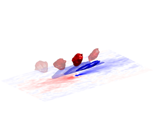
Backflow, namely the near-wall flow reversal is an extreme event occurring predominantly in the viscous sublayer where the instantaneous streamwise velocity becomes negative as illustrated in figure 1(a). The backflow received growing attention for its importance in the understanding of early stage flow separation, large-scale influence in the near-wall region and multiscale interaction in wall turbulence. The backflow manifests the penetration of structures in the buffer region and the logarithmic layer towards the wall, as a footprint of large-scale motions (LSMs) which have been reported to be responsible for the break-down of near-wall streaks (Falco Reference Falco1977), bursting events (Wark & Nagib Reference Wark and Nagib1991) and modulated near-wall activities (Mathis, Hutchins & Marusic Reference Mathis, Hutchins and Marusic2009).

Figure 1. (a) Typical instantaneous streamwise velocity profiles with near-wall backflow events from the present DNS data of pipe flows at  $Re_{\tau }=180$ (black), $Re_{\tau }=500$ (blue) and $Re_{\tau }=1000$ (red). (b) Locations of negative streamwise velocity (‘ $\blacksquare$’) in a single snapshot of the pipe at $Re_{\tau }=1000$.
The counter-intuitive existence of negative streamwise velocity in the vicinity of the wall under the significant mean shear was disputed (Eckelmann Reference Eckelmann1974). In the early observations of backflow, they were widely conceived as noises in experiments (Johansson Reference Johansson1988; Colella & Keith Reference Colella and Keith2003) and their genuine existence was not confirmed in experiments until the recent turbulent boundary layer (TBL) studies by Brücker (Reference Brücker2015), Willert et al. (Reference Willert2018) and Bross, Fuchs & Kähler (Reference Bross, Fuchs and Kähler2019). Direct numerical simulations (DNS) of canonical wall-bounded flows have reported the backflow in TBL (Spalart & Coleman Reference Spalart and Coleman1997; El Khoury et al. Reference El Khoury, Schlatter, Brethouwer and Johansson2014), channels (Hu, Morfey & Sandham Reference Hu, Morfey and Sandham2006; Lenaers et al. Reference Lenaers, Li, Brethouwer, Schlatter and Örlü2012; Cardesa et al. Reference Cardesa, Monty, Soria and Chong2014, Reference Cardesa, Monty, Soria and Chong2019; Chin et al. Reference Chin, Vinuessa, Örlü, Cardesa, Noorani, Schlatter and Chong2018a) and pipes (Chin et al. Reference Chin, Monty, Chong and Marusic2018b, Reference Chin, Vinuesa, Örlü, Cardesa, Noorani, Chong and Schlatter2020; Jalalabadi & Sung Reference Jalalabadi and Sung2018; Guerrero, Lambert & Chin Reference Guerrero, Lambert and Chin2020, Reference Guerrero, Lambert and Chin2022). The backflow was also investigated in the DNS of fully developed flows in ducts (Zaripov et al. Reference Zaripov, Ivashchenko, Mullyadzhanov, Li, Markovich and Kähler2021a,Reference Zaripov, Ivashchenko, Mullyadzhanov, Li, Markovich and Kählerb) and toroidal pipes (Chin et al. Reference Chin, Vinuessa, Örlü, Cardesa, Noorani, Schlatter and Chong2018a, Reference Chin, Vinuesa, Örlü, Cardesa, Noorani, Chong and Schlatter2020), and over wing sections (Vinuesa, Örlü & Schlatter Reference Vinuesa, Örlü and Schlatter2017; Zaki et al. Reference Zaki, Abdelrahman, Ayad and Abdellatif2022) where the backflow and the associated adverse pressure gradient (APG) led to flow separation on the wing. The backflow was also observed in turbulence transition by Wu, Cruickshank & Ghaemi (Reference Wu, Cruickshank and Ghaemi2020) in the late stage of bypass transition on a smooth, flat-plate boundary layer.
Consistent formation mechanism of the backflow and dynamics of the associated LSM were reported in the experiment (Bross et al. Reference Bross, Fuchs and Kähler2019) and DNS studies. The conditional average results by Lenaers et al. (Reference Lenaers, Li, Brethouwer, Schlatter and Örlü2012) showed that the backflow is formed at the upstream tail of a large-scale low-speed structure which is induced by a pair of counter-rotation quasi-streamwise vortices (Guerrero et al. Reference Guerrero, Lambert and Chin2020). A strong oblique spanwise vortex in the buffer region was observed above the backflow region (Lenaers et al. Reference Lenaers, Li, Brethouwer, Schlatter and Örlü2012; Vinuesa et al. Reference Vinuesa, Örlü and Schlatter2017; Bross et al. Reference Bross, Fuchs and Kähler2019; Guerrero et al. Reference Guerrero, Lambert and Chin2020; Zaripov et al. Reference Zaripov, Ivashchenko, Mullyadzhanov, Li, Markovich and Kähler2021a) as shown in the instantaneous fields around a backflow region in figure 2 with its swirl centre indicated by ‘ $\otimes$’ which resulted in a strong $Q4$ sweep region as marked in figure 2(a). The distribution of LSMs associated with the backflow corresponds to the organised vortices described by Adrian, Meinhart & Tompkins (Reference Adrian, Meinhart and Tompkins2000) where a large-scale low-speed structure is induced between the aligned legs of hairpin vortices which wrap around the low-speed structure with strong spanwise vortices as their heads along the inclined high-shear layer between the high- and low-speed structures (Guerrero et al. Reference Guerrero, Lambert and Chin2020; Zaripov et al. Reference Zaripov, Ivashchenko, Mullyadzhanov, Li, Markovich and Kähler2021a). The backflow and the accompanied extreme wall-normal velocity fluctuations near the wall are coupled with negative skin friction associated with APG as shown in figure 2(b). The spatiotemporal conditional average fields in Guerrero et al. (Reference Guerrero, Lambert and Chin2022) unfolded the evolution of the large-scale structures during the formation of backflow. The backflow was found to be a consequence of the ‘collision’ between the large-scale high- and low-speed structures which are the precursors of the backflow events. Before the occurrence of backflow, the oblique spanwise vortex was formed upstream at the trailing end of a large-scale low-speed structure which gradually diminished after the extreme events.

Figure 2. Contours around a backflow region (enclosed by the magenta contours of  $U=0$) in the instantaneous fields of (a) the inner-scaled wall-normal velocity fluctuation, $v^+$ in a close-up frame, and (b) the outer-scaled pressure fluctuation, $p$ from the present DNS data of the pipe at $Re_{\tau }=180$. The black lines in (a) are the streamlines of the mean flow, $U$ and $V$. The in-plane velocity fluctuations, $u$ and $v$ are indicated by vectors with swirl centres indicated by ‘ $\otimes$’.
The occurrence of the backflow events was quantified by Lenaers et al. (Reference Lenaers, Li, Brethouwer, Schlatter and Örlü2012) and Cardesa et al. (Reference Cardesa, Monty, Soria and Chong2019) in the channel and Guerrero et al. (Reference Guerrero, Lambert and Chin2020) in the pipe. As Reynolds number increased, the probability of the backflow events increased, and they appeared increasingly further away from the wall under inner scaling. The probability of the rare events was shown to be less than  $10^{-3}$ adjacent to the wall, and less than $10^{-5}$ outside the viscous sublayer for friction Reynolds numbers up to $Re_{\tau }\approx 2000$ (Cardesa et al. Reference Cardesa, Monty, Soria and Chong2019). Figure 1(b) marks all the identified backflow events in a single snapshot of the present pipe flow at $Re_{\tau }=1000$, unwrapped. The backflow events form scattered patches which we refer to as backflow structures in the study, and they are mostly attached to the wall. The shape of the backflow regions was found to be circular on the wall-parallel plane and semi-elliptical on the wall-normal plane by Lenaers et al. (Reference Lenaers, Li, Brethouwer, Schlatter and Örlü2012) with a resemblance to separation bubbles (Cardesa et al. Reference Cardesa, Monty, Soria and Chong2019) similarly shown by the backflow region outlined in figure 2. The results by Lenaers et al. (Reference Lenaers, Li, Brethouwer, Schlatter and Örlü2012), Vinuesa et al. (Reference Vinuesa, Örlü and Schlatter2017) and Cardesa et al. (Reference Cardesa, Monty, Soria and Chong2019) suggested that the average span of the backflow structures does not depend on the Reynolds number, scaling around 20 to 30 wall units in the wall-parallel directions, and only one wall unit in the wall-normal direction. The particle image velocimetry (PIV) study by Willert et al. (Reference Willert2018) suggested a consistent wall-parallel span of the backflow structures, but a noticeably larger wall-normal span of the backflow structures around five wall units, possibly due to the limited resolution of near-wall data acquirement.An overview of the commonly used measurement techniques for wall-shear stress was given by Örlü & Vinuesa (Reference Örlü and Vinuesa2020) which specifically addressed the capabilities and limitations of the experimental methods in the detection of backflow.
The average lifespan of the backflow structures was investigated in the channel, duct and boundary layers flows. Vinuesa et al. (Reference Vinuesa, Örlü and Schlatter2017) reported that the backflow structures had an average lifespan of  $T_{life}^+\approx 2$ over the wing section whereas the average lifespan of the backflow structures was found much longer in the duct and the channel. In Zaripov et al. (Reference Zaripov, Ivashchenko, Mullyadzhanov, Li, Markovich and Kähler2021b), the backflow structures had $T_{life}^+\approx 6$ in the core of the duct and lived even longer in the duct corner. They also showed that the lifespan of the backflow structures is positively correlated with their strength in which the longer-lived backflow structures can cause stronger flow reversal because they are associated with stronger vortical structures. The lifespan of the backflow structures in the channel was reported by Cardesa et al. (Reference Cardesa, Monty, Soria and Chong2014, Reference Cardesa, Monty, Soria and Chong2019) of $T_{life}^+\approx 7$. They trimmed the backflow structures with $T_{life}^+<2.4$ from the sample, which reduced the number of backflow structures by over $60\,\%$, yet only $6\,\%$ of the total volume of the backflow was reduced which indicated that the short-lived backflow structures are in general, much smaller.
The backflow structures are convected downstream by the mean flow with the large-scale structures, and the longer-lived backflow structures leave longer footprints on the wall (Zaripov et al. Reference Zaripov, Ivashchenko, Mullyadzhanov, Li, Markovich and Kähler2021b). Chin et al. (Reference Chin, Monty, Chong and Marusic2018b) estimated the travelling speed of a particularly long-living backflow structure (with  $T_{life}^+\approx 20$) of $U_m^+\approx 12$ in the pipe, which is notably faster than the average travelling speed suggested by Cardesa et al. (Reference Cardesa, Monty, Soria and Chong2014, Reference Cardesa, Monty, Soria and Chong2019) of $U_m^+\approx 9.4$ via time tracking of the backflow structures and the critical points of skin friction on the wall. Cardesa et al. (Reference Cardesa, Monty, Soria and Chong2019) suggested that the average travelling speed of the backflow structure coincided with the mean velocity in the buffer region and was similar to the convection speed of the near-wall streaks found by del Álamo & Jiménez (Reference del Álamo and Jiménez2009). The backflow structures were found to be travelling downstream at similar velocities of $U_m^+\approx 10.5$ in the core of the duct by Zaripov et al. (Reference Zaripov, Ivashchenko, Mullyadzhanov, Li, Markovich and Kähler2021b) and slightly faster in the corner, potentially due to the secondary motions in the duct corner. Despite the small discrepancies in the travelling speed of the backflow structures which may because of the difference in geometry, Reynolds number and estimation procedure, it is clear that the backflow structures carried by the large-scale structures travel at the mean flow velocities of the buffer region which is much faster than the mean flow in the viscous layer where they are largely immersed below $y^+=1$.
The evolution of the backflow structures was reported by Cardesa et al. (Reference Cardesa, Monty, Soria and Chong2019) who observed that the backflow structures became spanwise elongated during their growth. Their life stage conditional averaging results demonstrated the growth and decay of the backflow structures during their life cycle and showed that the longer-lived backflow structures can grow larger, i.e.extend further away from the wall and become more spanwise-elongated after growing to a certain wall-normal span. Their structure tracking and sorting method used following Lozano-Durán & Jiménez (Reference Lozano-Durán and Jiménez2014) suggested that the backflow structure split and merge at a negligible rate of  $2.7\,\%$ and $0.7\,\%$, respectively. They expected more of such behaviours in the APG TBL, though, in the earlier study by Vinuesa et al. (Reference Vinuesa, Örlü and Schlatter2017), no split or merged backflow structures were found in their APG TBL simulation. Cardesa et al. (Reference Cardesa, Monty, Soria and Chong2019) also reported that all the backflow structures were found to be wall-attached except for their $Re_{\tau }=2000$ case which had $0.04\,\%$ of the backflow structures identified away from the wall.
Exploration of the dynamics and evolution of the backflow will further complement our understanding of the large-scale influences in the near-wall phenomenon. In this study, we aim to further evaluate the statistical characteristics of the backflow structures including their size, lifespan, distribution density and travelling speed which few have been reported for the pipe and address possible Reynolds number trends. The relationships between the size, strength and lifespan of the backflow structures are examined. Particular efforts are paid to the evolution of the backflow structures. The inquired process of backflow structure splitting and merging is unveiled and investigated for possible causes including their interplay with the near-wall structures. At last, we explore the intriguing questions of whether a backflow structure can form detached from the wall and remain wall-detached during its whole life cycle, and what causes the wall-detached backflow structures which to the best of the authors’ knowledge, has not been investigated in either simulations or experiments.
2. Numerical methods
The present study is carried out on the DNS data of fully developed turbulent flows in the pipe and the channel at friction Reynolds numbers from  $Re_{\tau }=180$ to $1000$ as listed in table 1. The DNS data of the pipe are the same as in Chen, Chung & Wan (Reference Chen, Chung and Wan2020, Reference Chen, Chung and Wan2021). The incompressible Navier–Stokes equations are solved by the high-order spectral element method (SEM) in Nek5000 (Fischer, Lottes & Kerkemeier Reference Fischer, Lottes and Kerkemeier2008). The periodic boundary condition is applied in the streamwise direction of the pipe and the channel, and the spanwise direction of the channel, and the no-slip boundary condition is applied at all the walls. The streamwise and the wall-normal directions of the pipe and the channel are denoted as $x$ and $y$, respectively. The spanwise direction of the channel and the azimuthal direction of the pipe are denoted as $z$, and $\theta$ for the pipe, specifically. The streamwise length of the computational domain, $L_x=30\delta$ for both the pipe and the channel where the boundary layer thickness, $\delta$ is equivalent to the pipe radius, $R$, and the channel half height, $h$. The spanwise extent of the channel, $L_z=2{\rm \pi} h$ is the same as the circumferential length of the pipe wall. The streamwise domain is sufficiently long for the large-scale structures above the buffer layer with a well-established length of around $2\delta$ in the channel (del Álamo et al. Reference del Álamo, Jiménez, Zandonade and Moser2004; Lee et al. Reference Lee, Lee, Choi and Sung2014), pipe (Kim & Adrian Reference Kim and Adrian1999; Wu & Moin Reference Wu and Moin2008; Baltzer, Adrian & Wu Reference Baltzer, Adrian and Wu2013; Hellström, Ganapathisubramani & Smits Reference Hellström, Ganapathisubramani and Smits2015) and TBLs (Falco Reference Falco1977; Ganapathisubramani, Longmire & Marusic Reference Ganapathisubramani, Longmire and Marusic2003; Tomkins & Adrian Reference Tomkins and Adrian2003; Hutchins, Ganapathisubramani & Marusic Reference Hutchins, Ganapathisubramani and Marusic2004; Lee & Sung Reference Lee and Sung2013) and, therefore, should not affect the statistical results on the backflow caused by the large-scale structures inside and beyond the buffer region.
Table 1. The DNS parameters and the resolution of spatial and temporal discretisation of the present channel and pipe flows. Here  $N_s$ is the number of backflow structures identified in each flow case which includes both the top and the bottom walls of the channel.

Table 1 lists the parameters and resolutions of the dataset. In the spatial discretisation, the elements have a structured distribution in the channel and the streamwise direction of the pipe whereas the mesh on the cross-sections of the pipe is unstructured as shown in Wang et al. (Reference Wang, Örlü, Schlatter and Chung2018). Each of the hexahedral elements is refined by Gauss–Lobatto–Legendre (GLL) grid points with a Lagrange polynomial order of  $N=7$. The minimum wall-normal grid spacing $\Delta y$ in table 1 is located adjacent to the wall. The P1000 case with three billion grid points is performed with a preconditional algebraic multigrid solver in Nek5000 for scalability. For all the current simulations, the characteristic time scale is $\delta /U_b$ where the characteristic speed $U_b$ is the bulk mean velocity in the pipe and the channel. The dataset covers 60, 30 and 10 characteristic times in the fully turbulent state of the pipe and the channel for the cases of $Re_{\tau }=180$, $360\le Re _{\tau }\le 500$ and $Re_{\tau }=1000$, respectively, in the range of $690$– $880$ viscous times. The streamwise, wall-normal and spanwise/azimuthal velocities are denoted as $U$,
$U$,  $V$ and $W$, respectively, with capital letters for the instantaneous velocities, and the fluctuation terms expressed in lower cases.
3. Results and discussion
3.1. The occurrence of the backflow events
The probability of the instantaneous backflow events,  $\gamma$, as a function of wall distance is calculated as
 \begin{equation} \gamma(y)=\frac{1}{\Delta TL_xL_z}\int_{t_0}^{t_0+\Delta T}\int_{0}^{L_x}\int_{0}^{L_z}\varGamma\,\mathrm{d}z\,\mathrm{d}x\,\mathrm{d}t, \end{equation}
where  $\Delta T$ is the integration time length, and $\varGamma (x,y,z)$ is a logical function of whether a data point has a backflow event, i.e. $U<0$. In figure 3(a), the distributions of $\gamma$ from the present channels and pipes all show good agreement with the previous DNS results in which the probability of the backflow events decreases monotonically away from the wall, and they appear further away from the wall at higher Reynolds numbers. The velocity profiles conditionally averaged at the backflow events, i.e.the mean velocity profiles of the backflow regions are plotted in figure 3(b). The velocity profiles of the higher-Reynolds-number cases are not very smooth for $y^+>3$ because of the low sampling rate, $\gamma$. The inner-scaled velocity profiles of the backflow structures are fairly collapsed for $Re_{\tau }\ge 360$, suggesting that the backflow structures at moderate- to high-Reynolds-number flows are similar in size and strength. In the subset, the parabolic mean velocity profiles of the backflow structure indicate that the strongest flow reversal is roughly at the centre of the backflow structures which is also suggested by the instantaneous velocity profiles in figure 1(a). The results in figure 3 suggest that the probability of the backflow events and the mean velocity profile in the backflow regions are very similar in the pipe and the channel.
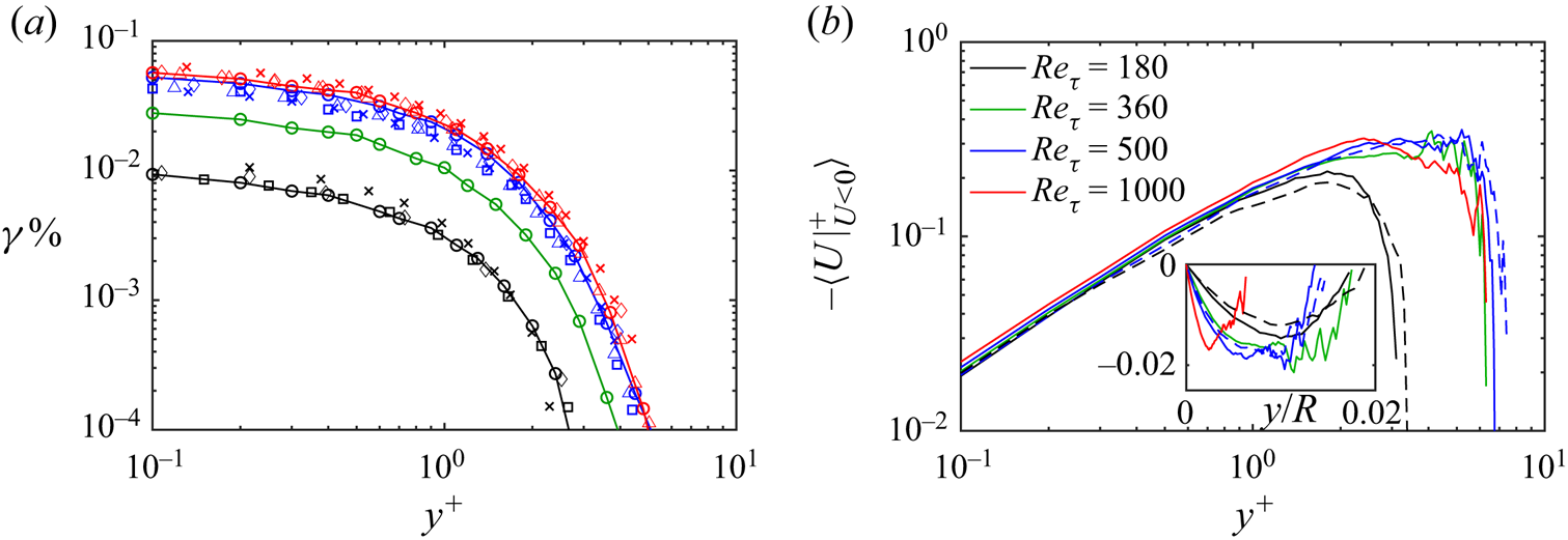
Figure 3. (a) Percentage of backflow events vs wall distance for the present pipe (solid lines and ‘ $\bigcirc$’) and channel (‘ $\square$’) data. Overlaid are the DNS results of the channel by Lenaers et al. (Reference Lenaers, Li, Brethouwer, Schlatter and Örlü2012) (‘ $\lozenge$’) at $Re_{\tau }\approx 180$, 585 and 1000, and Cardesa et al. (Reference Cardesa, Monty, Soria and Chong2019) (‘ $\vartriangle$’) at $Re_{\tau }\approx$ 550 and 950 and the pipe by Guerrero et al. (Reference Guerrero, Lambert and Chin2020) (‘ $\times$’) at $Re_{\tau }\approx 170$, 500 and 1000. (b) The time-averaged streamwise velocity profiles computed from locations with backflow events in the pipe (—–) and the channel ( $---$).
3.2. The formation of backflow and the dynamics of the large-scale structures
The volumetric conditional average fields indicated by  $\langle \cdot \rangle$ around the backflow events with their location denoted with a hat ( $\hat {x}$, $\hat {\theta }$, $\hat {y}$) are shown in figure 4. The large-scale high- and low-speed structures associated with the backflow are shown by the isosurfaces of $\langle u\rangle$ with the contours of $\langle u\rangle$ on the mid-plane of the coherent structures at $\hat {\theta }$. The fluctuating wall shear stress is presented by the fluctuation of skin friction coefficient, $c_f=2\tau _w/(\rho U_c^2)$ where $U_c$ is the centreline velocity. The backflow takes place at the tail tip of the low-speed structure with the typical length scale of LSM. The high-speed region above the backflow was observed to be pushed towards the wall by the strong spanwise vortex (Lenaers et al. Reference Lenaers, Li, Brethouwer, Schlatter and Örlü2012; Vinuesa et al. Reference Vinuesa, Örlü and Schlatter2017; Bross et al. Reference Bross, Fuchs and Kähler2019; Zaripov et al. Reference Zaripov, Ivashchenko, Mullyadzhanov, Li, Markovich and Kähler2021a). The backflow is also accompanied by a thin upstream near-wall high-speed layer which couples to a region of high skin friction whereas the large low-speed structure results in a streamwise-elongated region of negative skin friction (Vinuesa et al. Reference Vinuesa, Örlü and Schlatter2017). The sudden variation of skin friction at the critical point of zero wall shear stress under the backflow events has been reported by Brücker (Reference Brücker2015) and Chin et al. (Reference Chin, Monty, Chong and Marusic2018b, Reference Chin, Vinuesa, Örlü, Cardesa, Noorani, Chong and Schlatter2020).

Figure 4. The isosurfaces of  $\langle u\rangle$ in the conditionally averaged fields around the backflow events in the pipe at $Re_{\tau }=1000$, and the two-dimensional contour of $\langle u\rangle$ on the mid-plane of the large-scale structures at $\hat {\theta }$ plotted at the back. The contour of the conditional average skin friction fluctuation on the wall, $c_f'$ is plotted at the bottom.
The dynamics of the large-scale structures are evaluated by means of spatiotemporal conditional averaging similar to Guerrero et al. (Reference Guerrero, Lambert and Chin2022), centring the backflow events at  $(\hat {x}, \hat {\theta }, \hat {y}, \hat {t})$ where $\hat {t}$ is the time of the events. Figure 5(a,b) show the time track of the low-speed structure with ejection events and the high-speed structure with sweep events, respectively, and the interaction between the large-scale structures is illustrated in figure 5(c). A few characteristic times before the backflow is formed, the low-speed structure appears adjacent to the wall, and the large high-speed region which originates upstream of the low-speed structure (Zaripov et al. Reference Zaripov, Ivashchenko, Mullyadzhanov, Li, Markovich and Kähler2021a) is distant from the wall in the log-law region. The low-speed structure is convected along the wall and concurrently, the patch of high-speed fluids is swept towards the wall by the vortical structures (Lenaers et al. Reference Lenaers, Li, Brethouwer, Schlatter and Örlü2012; Bross et al. Reference Bross, Fuchs and Kähler2019; Zaripov et al. Reference Zaripov, Ivashchenko, Mullyadzhanov, Li, Markovich and Kähler2021a). The high-speed structure is convected downstream naturally faster than the low-speed structure and they ‘collide’ as described in Guerrero et al. (Reference Guerrero, Lambert and Chin2022) when the backflow events take place underneath the high-speed structure at the tail tip of the low-speed structure where it has become strong enough to overcome the mean shear. The observed dynamics of the large-scale structures are consistent with Guerrero et al. (Reference Guerrero, Lambert and Chin2022), and are presented in the supplementary movie available at https://doi.org/10.1017/jfm.2023.461. With indication from the size of the high- and low-speed region in figure 5, both the high- and low-speed structures remain in strength as precursors of the backflow until it is formed, and rapidly weaken after the backflow events.

Figure 5. Time tracks of the large-scale high- and low-speed structures around the backflow events in the spatiotemporal conditional averaged fields around the backflow events at ( $\hat {x}, \hat {\theta }, \hat {y}, \hat {t}$) in the pipe at $Re_{\tau }=1000$. The contours of $\langle u\rangle$ and $\langle v\rangle$ are plotted in (a) for $Q2$ ejection events ( $u<0,\ v>0$) and (b) for $Q4$ sweep events ( $u>0,\ v<0$). The three-dimensional isosurfaces correspond to the solid contours of $\langle u\rangle$. (c) Contours of the low-speed structure (thick lines) and the high-speed structure (thin lines), i.e.the solid contours in (a,b) displayed together.
Figure 6 shows the in-plane velocity fluctuations on a cross-stream plane moving downstream at  $U_b$ which follows and cuts through the high-speed structure. The location and the time of the frames are indicated on the horizontal axes with frames I and II labelled corresponding to figure 5(c). Here we show that the high-speed structure is continuously swept towards the wall by a pair of inward counter-rotating streamwise vortices beyond the buffer region which continuously push the high-speed structure onto the trailing end of the low-speed structure. After the backflow event, this pair of persistent vortices continue to push the large patch of high-speed fluids onto the wall to replace the low-speed structure and the associated negative skin friction before it diminishes, i.e.a successive penetration of large-scale low- and high-speed fluids into the viscous wall region.

Figure 6. Contours of the streamwise fluctuation  $u$ in the spatiotemporal fields conditionally averaged around the backflow events in the pipe at $Re_{\tau }=1000$. The contours are drawn on a cross-stream plane at varying streamwise locations moving downstream at $U_b$, cutting through the high-speed structure shown in figure 5. The in-plane fluctuations, $\langle v\rangle$ and $\langle w\rangle$ are shown by vectors, and the swirl centres are marked by ‘ $\otimes$’.
3.3. Characteristics of the backflow structures
The later part of this study investigates the backflow as individual dynamical structures with varying lifespans. The instantaneous backflow events are grouped into clustered backflow structures by examining the spatial and temporal connections between the spatial location and time of occurrence of all the backflow events at discrete grid points. The identification is schematically demonstrated by a single backflow structure in figure 7. For each collocation point with  $U<0$, it is tagged as the same backflow structure with all the other adjacent backflow events located at the neighbouring points in three dimensions similar to Cardesa et al. (Reference Cardesa, Monty, Soria and Chong2019) and a similar rule is applied temporally. As demonstrated in figure 7(c), the instantaneous clusters of backflow events are grouped if they have spatial overlap between successive snapshots. In other words, the backflow events which are ‘connected’ spatiotemporally are recognised as the same structure. Such connections are based on the assumption that the computational grid spacing and the time gap between snapshots are sufficiently refined to resolve and track the backflow structures being convected downstream which is remarked at the end of § 3.3.

Figure 7. Illustration of the identification of backflow structures from instantaneous backflow events. (a) The locations of a backflow structure in three successive snapshots where  $t_s$ is the uniform time gap between snapshots. (b,c) Streamwise and top views of (a), respectively, indicating the overlapped locations of the instantaneous backflow regions.
3.3.1. The distribution density of the backflow structures
The total number of independent backflow structures identified in each case,  $N_s$, is presented in table 1. Figure 8(a–c) show all the backflow structures identified over the period for the mean flow to pass the fixed streamwise domain $L_x$ of the pipe at $Re_{\tau }=180$ and 360. Although figure 3(a) has already shown that the occurrence of the backflow events increases with the Reynolds number, it is more perceivable here how significantly more backflow structures occur with increasing Reynolds numbers. These backflow structures are plotted for their whole lifespan as a superposition of their instantaneous distributions like footprints so that in figure 8(c), the more streamwise-elongated objects indicate backflow structures with longer lifespans, being convected downstream similar to Zaripov et al. (Reference Zaripov, Ivashchenko, Mullyadzhanov, Li, Markovich and Kähler2021b) (see their figure 5). Figure 8(d) shows the distribution density of the backflow structures in the present pipes and channels, i.e.the average number of backflow structures per million wall square units, $n_A^+$ with the channel results from Cardesa et al. (Reference Cardesa, Monty, Soria and Chong2019). The channel results suggest that there are slightly more backflow structures in an inner-scaled unit area of the channel wall compared with the pipe. The results indicate that at $Re_{\tau }=1000$, over one characteristic time length for which the bulk flow at $U_b$ has convected downstream over $1\delta$, there will be over three backflow regions occurring in a squared area of $\delta ^2$ on the wall and, hence, on average, 20 backflow structures will occur on the circumferential pipe wall for the bulk flow passing $1\delta$ downstream. The distribution density of the backflow structures increases monotonically with the Reynolds number where the increase becomes gradual, showing signs of convergence towards higher Reynolds numbers, though it would require further data at much higher Reynolds numbers to confirm possible Reynolds number independence of $n_A^+$.

Figure 8. (a–c) The backflow structures occurred during the time for the bulk flow to pass over the domain in (a) at  $Re_{\tau }=180$, (b) at $Re_{\tau }=360$, coloured based on their time of appearance, and (c) is the wall-normal view of (b). (d) The average number of backflow structures per million wall square units, $n_{A}^+$, and per outer square unit ( $\delta ^2$) of the wall. (e) Percentage of the contact area of the backflow region on the wall per characteristic time.
An important indication from the temporally superpositioned footprints of the backflow structures in figure 8(a–c) is that the extremely rare backflow events with probabilities below  $10^{-3}$ at the wall instantaneously can, in fact, leave the wall fully covered by the imprints of backflow in time when we evaluate the impact of the extreme events on the wall in a long time frame in engineering applications. Figure 8(e) shows the percentage of average wall area that has been under the backflow region per characteristic time, $\psi$ which accounts for not only the number of backflow structures on the wall ( $n_A$) but also their lifespan (a longer-lived backflow region imprints more area of the wall in time) and the contact area between the backflow structure and the wall, i.e. the wall-parallel span of the backflow structure. The distribution of $\psi$ indicates that in a given time, the flows at higher Reynolds numbers will have a larger part of the wall to experience backflow which was expected from the results in figure 8(d). The results indicate that at $Re_{\tau }=1000$, the footprints from the backflow structures occupy an area of nearly $0.6\,\%$ of the wall after the bulk flow has passed for $1\delta$, in other words, the flow can have the wall fully covered by the footprints of backflow in a period of $170\delta /U_b$ at $Re_{\tau }=1000$ on average, and in an increasingly shorter time as Reynolds number increases.
3.3.2. The scale, lifespan and strength of the backflow structures
In the life cycle of a backflow structure, the size of the structure increases and decreases during its growth and decay (Cardesa et al. Reference Cardesa, Monty, Soria and Chong2019). In this study, the ‘matured’ stage of a backflow structure refers to the structure at its largest form with its maximum volume  $\mathcal {V}$ in which the calligraphic font indicates the maximum measurements of a backflow structure during its lifetime throughout this study. Figure 9 shows the maximum instantaneous span of the backflow structures in the spanwise, streamwise and wall-normal directions of the pipe and the channel, $\mathcal {D}z$ (or $\mathcal {D}\theta$ for the pipe), $\mathcal {D}x$ and $\mathcal {D}y$ in wall units. The average span of the matured backflow structures in the present pipe and channel lies in the range reported for canonical wall-bounded flows which consistently suggests that $\mathcal {D}x^+$ and $\mathcal {D}z^+$ are approximately 20 wall units and $\mathcal {D}y^+\approx 1$. The average wall-parallel spans of the matured backflow structures increase slightly with the Reynolds number as shown in Zaripov et al. (Reference Zaripov, Ivashchenko, Mullyadzhanov, Li, Markovich and Kähler2021a) (their figure 4b) whereas the average wall-normal extent, i.e. the height of the backflow structures is independent of Reynolds number (Lenaers et al. Reference Lenaers, Li, Brethouwer, Schlatter and Örlü2012; Cardesa et al. Reference Cardesa, Monty, Soria and Chong2019; Zaripov et al. Reference Zaripov, Ivashchenko, Mullyadzhanov, Li, Markovich and Kähler2021a).

Figure 9. The average span of the backflow structures in the spanwise (magenta) and streamwise (blue) directions on the left axis, and in the wall-normal direction (black) on the right axis for the present pipe (‘ $\bigcirc$’) and channel (‘ $\square$’), overlapped with the results by Lenaers et al. (Reference Lenaers, Li, Brethouwer, Schlatter and Örlü2012) (‘ $\lozenge$’), Jalalabadi & Sung (Reference Jalalabadi and Sung2018) (‘ $\triangledown$’), Cardesa et al. (Reference Cardesa, Monty, Soria and Chong2019) (‘ $\vartriangle$’) and Zaripov et al. (Reference Zaripov, Ivashchenko, Mullyadzhanov, Li, Markovich and Kähler2021a) (‘ $+$’). (b) The average lifespan of the backflow structures.
The average lifespan of the backflow,  $T_{life}$ is found to be around 8 wall units. In figure 9(b), the pipe results are very similar to the TBL results by Brücker (Reference Brücker2015) whereas $T_{life}$ is found slightly lower in our channel, similar to Cardesa et al. (Reference Cardesa, Monty, Soria and Chong2014, Reference Cardesa, Monty, Soria and Chong2019). The relationships between the lifespan, the strength, and the size of the backflow structures are explored. Here, the strength of the backflow structure is simply defined by the most negative streamwise velocity in the backflow region during its lifetime, denoted as $\mathcal {U}$. Intuitively, a backflow structure with a longer lifespan would enable the structure to become larger (Cardesa et al. Reference Cardesa, Monty, Soria and Chong2019) and stronger (Zaripov et al. Reference Zaripov, Ivashchenko, Mullyadzhanov, Li, Markovich and Kähler2021b). However, the joint probability density distribution (p.d.f.) in figure 10(a) suggests that although the backflow structures with longer lifespans can achieve stronger flow reversal on average, the rare outstandingly long-lived backflow structures with lifespans more than three times longer than the average ( $T_{life}^+>30$) are not necessarily even stronger. In figure 10(b), the joint p.d.f. between the lifespan and the maximum size of the backflow structure shows a similar distribution where the outstandingly long-lived backflow structures are not the largest in the flow on average. Figure 10(c) shows the relationship between the strength and the size of the backflow structure. The size and the strength of the backflow structure are positively correlated with each other with a Pearson correlation coefficient higher than 0.7 for all the flow cases. The results in figure 10 suggest that the backflow structures are stronger and larger with longer lifespans up to a certain point in which the outstandingly long-lived backflow structures with a lifespan $3$–
$3$– $4$ times longer than the average in a given flow, are unlikely to be the largest and strongest ones in the flow.

Figure 10. Joint p.d.f.s between (a) the strength of the backflow structures, and the lifespan of the backflow structures,  $T_{life}$, (b) $T_{life}$ and the maximum volume of the backflow structures, $\mathcal {V}$, and (c) $\mathcal {V}$ and $\mathcal {U}$ in the pipe at $Re_{\tau }=500$ (colour-filled contours) and 1000 (isocontour lines).
After a close examination of the particularly large and the particularly long-lived backflow structures, it is found that although the backflow structures need a certain lifespan to develop in size and strength, it is uncommon for those backflow structures with outstandingly long lifespans to continuously expand. Figure 11 shows a selection of the extremely long-lived backflow structures with  $T_{life}^+\approx 50$ which are much longer-lived compared with the long-lived backflow reported by Chin et al. (Reference Chin, Monty, Chong and Marusic2018b) and Zaripov et al. (Reference Zaripov, Ivashchenko, Mullyadzhanov, Li, Markovich and Kähler2021b) with $T_{life}\approx 20$ and Bross et al. (Reference Bross, Fuchs and Kähler2019) with $T_{life}\approx 28$. The backflow structures are visualised in the streamwise–spanwise–temporal space with their time track shown by their temporal and spanwise projections. The backflow is initially round (Lenaers et al. Reference Lenaers, Li, Brethouwer, Schlatter and Örlü2012) and small, which grows larger in time and elongates in the spanwise direction as observed by Cardesa et al. (Reference Cardesa, Monty, Soria and Chong2019). The backflow structure in figure 11(a) shows a rare example among the outstandingly long-lived backflow structures which goes through a life cycle of growth and decay as a typical backflow structure. Instead of continuous growth, the outstandingly long-lived backflow structures are much more commonly found to be going through multiple cycles of growth and decay as shown in figure 11(b,c), possibly due to the regeneration cycle (20–30 wall units in time) of the organised vortices in the buffer region inducing LSMs and the backflow (Jodai & Elsinga Reference Jodai and Elsinga2016). The fact that the backflow structures cannot continuously grow larger with an extremely long lifespan is also because of the splitting of backflow structures which is investigated in § 3.4.1. We expect the strength and the size of the backflow structures to be positively correlated with their lifespan when the outstandingly long-lived backflow structures are further sorted based on the life cycle.

Figure 11. Temporal evolution of the backflow structures with outstandingly long lifespans in the pipe at  $Re_{\tau }=360$, visualised by the trace of the backflow structures on the wall-parallel plane along the time axis with spatiotemporal projections.
3.3.3. The travelling velocity of backflow structures
The travelling velocities of the backflow structures are measured as illustrated in figure 12. On the streamwise–temporal map, the isolated black filaments are the streamwise traces of individual backflow structures which are visibly convected downstream at a similar velocity at each Reynolds number. For each of the backflow structures, its streamwise movement is estimated by  $\tilde {x}=U_mt+\tilde {x}_0$ where $U_m={\rm d}\,\tilde{x}/{\rm d}t$ is the estimated travelling speed of the backflow structure and $\tilde {x}_0$ is the estimated initial streamwise location of the structure. The linear estimation for each backflow structure is indicated by the magenta lines along each backflow structure in figure 12, and the grey lines in the background indicate the average travelling velocity of the backflow structures at each Reynolds number, $\bar {U}_m$.

Figure 12. The streamwise locations and the time of occurrence of the backflow events, plotted on the streamwise–temporal map for the pipe flow at (a)  $Re_{\tau }=180$, (b) $Re_{\tau }=360$ and (c) $Re_{\tau }=500$. Only $1/4$ of the backflow structures in the $Re_{\tau }=500$ case are shown for clarity. The magenta lines are the first-degree best fits for the travelling speed $\alpha$ of individual structures, $\tilde {x}=\alpha t+\tilde {x}_0$ where $\tilde {x}_0$ is the initial streamwise location of each structure. The grey lines represent the average travelling speed, $\overline {{\rm d}\tilde {x}/{\rm d}t}$ at each Reynolds number while the cyan lines represent a travelling speed at $U_b$.
In figure 13, the inner-scaled average travelling velocity of the backflow,  $U_m^+$ lies reasonably in the range of $U_m^+$ suggested by Cardesa et al. (Reference Cardesa, Monty, Soria and Chong2019) and Zaripov et al. (Reference Zaripov, Ivashchenko, Mullyadzhanov, Li, Markovich and Kähler2021b). The 10 % difference between the channel results by Cardesa et al. (Reference Cardesa, Monty, Soria and Chong2019) and the present results is potentially caused by the difference in the estimation procedure of $U_m$ rather than the difference between pipe and channel since the present pipe and channel results are remarkably similar to each other. The backflow is convected downstream at the mean streamwise velocities corresponding to the buffer region as reported by Cardesa et al. (Reference Cardesa, Monty, Soria and Chong2019), similar to the travelling velocities of the precursory large-scale low-speed structures which travel around $0.6U_b$ at $Re_{\tau }=1000$, estimated from figure 5(c). Although the backflow structures are on average, confined within $y^+=1$, they are convected much faster than the mean velocities of the viscous layer because they are carried by the large low-speed structure originating from the buffer layer and pushed by the large-scale high-speed structures originated beyond the buffer layer (Lenaers et al. Reference Lenaers, Li, Brethouwer, Schlatter and Örlü2012; Vinuesa et al. Reference Vinuesa, Örlü and Schlatter2017; Bross et al. Reference Bross, Fuchs and Kähler2019; Cardesa et al. Reference Cardesa, Monty, Soria and Chong2019; Zaripov et al. Reference Zaripov, Ivashchenko, Mullyadzhanov, Li, Markovich and Kähler2021a; Guerrero et al. Reference Guerrero, Lambert and Chin2022). The trend of $U_m^+$ in figure 13 also suggests a subtle increase in the convection speed of the backflow structures with increasing Reynolds number.

Figure 13. The average travelling speed of backflow structures in the pipe (‘ $\bigcirc$’) and the channel (‘ $\square$’), estimated as shown in figure 12, and overlapped with the average results from the channel by Cardesa et al. (Reference Cardesa, Monty, Soria and Chong2019) (‘ $\vartriangle$’) and the core region of the duct by Zaripov et al. (Reference Zaripov, Ivashchenko, Mullyadzhanov, Li, Markovich and Kähler2021b) (‘ $*$’), and for a single long-lived backflow structure in the pipe by Chin et al. (Reference Chin, Monty, Chong and Marusic2018b) (‘ $\unicode{x2730}$’).
3.4. Evolution of backflow structures
3.4.1. The splitting and merging of backflow structures
The causes of the splitting and merging of backflow regions during their evolution are investigated. Figure 14 illustrates the identification of the split and merged backflow structures. The temporal projections of the backflow structures on the wall-parallel plane are used to identify their splitting and merging. As shown in figure 14(a), the split and merged backflow structures result in ‘swallowtail’-shaped temporal projections on the wall-parallel plane. Figure 14(b) shows a typical ‘swallowtail’-shaped temporal projection of the split and merged backflow structures. For each backflow structure, all the instantaneous spatial gaps between the backflow events are noted. For a splitting structure, the instantaneous spatial gap between the backflow events appears in the downstream end of the projection, i.e.in the latter part of the lifespan of the backflow, and is the opposite for a merging structure as illustrated in figure 14(b). It is worth noting here that a merged or a split backflow structure is counted as one backflow structure, though they are negligible in affecting the statistical results such as  $n_A$ since they occur at extremely low rates (Cardesa et al. Reference Cardesa, Monty, Soria and Chong2019).

Figure 14. (a) The backflow structures identified over a period in the pipe at  $Re_{\tau }=180$, plotted in the streamwise–azimuthal–temporal space with temporal projections on the streamwise–azimuthal plane. The identified split backflow structures are highlighted in red. (b) Illustration of the identification of merging and splitting backflow structures.
The overall percentage of the split and merged backflow structures in the dataset is found to be very similar to Cardesa et al. (Reference Cardesa, Monty, Soria and Chong2019) at approximately  $3\,\%$ and $0.8\,\%$, respectively. The merged backflow structures are extremely rare in which none is obtained in the channel and pipe at $Re_{\tau }=180$ because of the limited sample size $N_s$. A selection of representative backflow structures with splitting, merging and other peculiar evolutions is shown in figure 15. In figure 15(a), two extremely small backflow regions appear near each other roughly at the same time. The two small backflow regions grow particularly along the spanwise direction (Cardesa et al. Reference Cardesa, Monty, Soria and Chong2019) until they are connected in the spanwise direction and merge into one. After merging, the spanwise-elongated backflow region continues to grow and eventually decays and diminishes. A backflow structure does not necessarily merge when it has separated backflow regions near each other as shown in figure 15(b) with two backflow regions residing extremely close to each other and remaining separated during their whole life cycle. A typical split backflow structure is shown in figure 15(c). The backflow structure is initially formed round and small as a ‘normal’ backflow structure which split after it has become larger and spanwise-elongated. After splitting, its split parts gradually diminish without undergoing new life cycles unlike in figure 15(d) with a regenerated backflow structure from a split part which undergoes a second life cycle of growth and decay and splits again. It is observed from the split backflow structures that they tend to split in the spanwise direction whereas they do not seem to split in the streamwise direction, and they become notably elongated in the spanwise direction before they split.

Figure 15. Temporal evolution of the backflow structures in the pipe at  $Re_{\tau }=360$ exhibiting splitting and merging behaviours, visualised by the trace of the backflow structures on the wall-parallel plane along the time axis with spatiotemporal projections.
The cause of the splitting of backflow regions is examined by computing the maximum instantaneous wall-parallel span of the backflow,  $\mathcal {D}x$ (or $\mathcal {D}\theta$) and $\mathcal {D}z$, averaged for the split backflow which is compared with the average span of the whole sample (figure 9). Figure 16(a) shows that the split backflow structures have larger wall-parallel spans and are more elongated in the spanwise direction on average. The evolution of a backflow structure is schematically illustrated in figure 16(b), showing its chance of splitting is largely affected by its spanwise extent. The larger and more spanwise-elongated backflow structures are more likely to split owning to the near-wall structures, tearing apart the backflow structures that are large enough to span over the high- and low-speed streaks near the wall. In figure 16(a), the typical spanwise spacing between the high- and low-speed streaks is represented by the dot-dashed line of $\delta z^+=50$ (Smith & Metzler Reference Smith and Metzler1983; Kim, Moin & Moser Reference Kim, Moin and Moser1987). It is clear that the average spanwise extent of the split backflow regions is larger than the spacing between the near-wall streaks so that they span over the near-wall streaks and are split by the high- and low-speed streaks.

Figure 16. (a) The maximum instantaneous span of the backflow structures in the spanwise direction,  $\mathcal {D}z$ (magenta) and in the streamwise direction, $\mathcal {D}x$ (blue), averaged for all the backflow structures (empty symbols) and the split backflow structures only (solid symbols) in the pipe ( $\bigcirc$) and the channel ( $\square$). (b) A schematic comparison of the evolution between the normal backflow structures and the split backflow structures.
The dynamics of the distortion of the backflow region by the near-wall streaks is presented in figure 17 by the temporal evolution of the backflow on the instantaneous contour of  $U$ at five life stages of the structure. The high-speed streaks around the backflow are marked with ‘hs’. In figure 17(b), shortly before the backflow is formed, the three high-speed streaks are isolated and the tail of hs-2 is much weaker than hs-1 under the influence of the large low-speed structure indicated by the enclosed dashed line with a typical length scale of the LSMs. After forming, the backflow structure grows in size, particularly in the spanwise direction which spans over hs-2, and the two low-speed streaks on either side of hs-2 in the middle of its lifespan and is on the verge of splitting. In figure 17(f), as the backflow and the associated large-scale structures start to decay, hs-1 and hs-2 have been connected and the backflow structure has been split by the local distortion from the spanwise shearing due to the near-wall streaks, seemingly divided by hs-1 and hs-2.

Figure 17. (a) The temporal evolution of the split backflow structure shown in figure 15(c) on the streamwise-spanwise plane. The contours of instantaneous streamwise velocity  $U$ at $y^+=1$ are plotted at different life stages of the lifespan of the backflow. The black outline in (c–f) is the time track of the dynamic structure and the instantaneous backflow in each frame is outlined in the colour magenta.
Observations suggest that the near-wall streaks are also responsible for the merging and separation of backflow regions. Figure 18(a–c) show the temporal evolution of the separated backflow shown in figure 15(c). The backflow is formed at the two sides (BF-a and BF-b) at the tail tip of the low-speed structure, separated by the remnant of the high-speed streak (hs-1) broken down by the low-speed structure. After the backflow is formed, hs-1 is seen to be recovering in strength and keeps the backflow structure separated in figure 18(b) where the backflow should have grown to its matured size so that a larger part of the tail of the low-speed structure becomes sufficiently strong for flow reversal, which explains the short appearance of BF-c. BF-c is also isolated from the other two backflow regions due to the obstruction of hs-1, and these separated small backflow regions never merge into one large backflow structure until it diminishes. Similarly, the backflow structure in figure 18(d–f) is initially formed flanked at the tail tip of the low-speed structure with the vanishing remnant of a high-speed streak in between. As the backflow develops, the two offspring backflow merge and become the spanwise-elongated backflow structure in figure 18(e). The results indicate that the near-wall high- and low-speed streaks are responsible for the splitting, separation and merging of the backflow. They play an important role in the evolution of backflow regions, i.e.the formation of separated backflow regions and whether the backflow structures can merge or not during their lifetime.

Figure 18. The temporal evolution of (a–c) the separated backflow structure in figure 15(c) and (d–f) the merged backflow structure in figure 15(a) on the streamwise-spanwise contours of instantaneous streamwise velocity  $U$ at $y^+=1$ at different life stages of the backflow structures (in the colour magenta).
3.4.2. The wall-detached backflow structures
Another intriguing question regarding the evolution of the backflow is whether a backflow region can appear away from the wall and remain detached from the wall during its whole life cycle. This section presents evidence of the wall-detached backflow regions and elucidates their formation dynamics. The wall-detached backflow structures are identified by examining each of the backflow structures for whether its instantaneous distribution is absent from the first layer of the grid adjacent to the wall. Based on the life stage for a backflow structure that is detached from the wall, it is categorised into three types: (i) detached in the front part of its lifespan, (ii) detached for its whole lifespan and (iii) detached in the rear of its lifespan as demonstrated in figure 19. No backflow structure departing away from the wall is encountered in our dataset and type (iii) is excluded from wall-detached backflow structures based on the observation that it is the natural decaying process of backflow regions where they can leave their strongest core region at the very end of their lifespan. Thus, in the later discussion, only the backflow structures initially formed away from the wall, i.e. types (i) and (ii) are referred to as the wall-detached backflow structures, which appear at a probability of around 0.2 % when estimated from the whole dataset.

Figure 19. Schematic illustration of the types of wall-detached backflow structures.
The life cycle of the wall-detached backflow structures is depicted in figure 20 which provides the first visualisation of wall-detached backflow. It is shown that the wall-detached backflow always tends to become wall-attached by approaching the wall which is the case for both types (i) and (ii) as schematically illustrated in figure 19, in fact, type (ii) backflow regions are essentially the same as type (i) but having an insufficient lifespan to reach the wall. While approaching the wall, the backflow regions initially formed away from the wall go through the normal life cycle of backflow with growth and decay, and continue this process after reaching and resting on the wall. Furthermore, by examining the instantaneous skin friction under the wall-detached backflow regions, we found that there is no critical point of zero shear stress under the wall-detached backflow until it arrives at the wall.

Figure 20. Temporal evolution of backflow structures formed away from the wall of (a) type (ii), (b) type (i) and (c) type (i) with merging and splitting in the pipe at  $Re_{\tau }=360$, visualised in three-dimensional space with spatiotemporal projections.
Having observed the existence and life cycle of backflow forming detached from the wall, we investigate their cause and if there is any difference in their formation mechanism compared with the wall-attached backflow structures. The wall-detaching of backflow appears to be caused by the near-wall high-speed streaks which separate the tail tip of the large-scale low-speed structure and the wall with a thin layer of positive streamwise velocity. The temporal evolution of the backflow region initially appeared at  $y^+>2$ shown in figure 20(a) is displayed on the wall-parallel and the streamwise–wall-normal contours of $u$ in figure 21 to demonstrate the formation mechanism of wall-detached backflow. The formation of the wall-detached backflow is similar to a normal backflow region on the wall which forms at the tail tip of a large-scale low-speed structure beneath the strong downwash of high-speed fluids, yet away from the wall because the tail tip of the carrier low-speed structure ‘sits’ on the high-speed streak marked with ‘hs-a’. The downstream part of the low-speed LSM is also kept away from the wall by the high-speed streak ‘hs-b’. The formation dynamics are found similar to all the wall-detached backflow regions resolved in at least three consecutive snapshots, forming away from the wall when the tail of the low-speed structures is obstructed by the near-wall high-speed streaks during their formation. As discussed in § 3.2, the large-scale high-speed structure is continuously swept down towards the wall by the vortical structures in the buffer region, and it pushes the tail of the low-speed structure onto the wall so that the wall-detached backflow regions always tend to attach to the wall during their life cycle and, thus, it is unlikely for a wall-attached backflow region to detach away from the wall.

Figure 21. The temporal evolution of the backflow structure initially formed detached from the wall in figure 20(b) on the streamwise wall-parallel and wall-normal contours of instantaneous streamwise fluctuation  $u$ at $y^+=1$ at $(t-t_0)/T_{life}\approx 0.1$ in (a), 0.3 in (b), 0.5 in (c) and 0.9 in (d). On the wall-parallel plane, the backflow structure is indicated by the magenta contour of $U=0$ if in presence at $y^+1$ and is otherwise indicated by a filled shape taken from where it is in presence, in this case $y^+\approx 2$, and overlapped on the contour of $u$ at $y^+=1$.
Given that the wall-detached backflow is also caused by the near-wall high-speed streaks which obstruct the large-scale low-speed structures, similar to the splitting and merging of backflow discussed in § 3.4.1, the backflow presented in figure 22 is a fascinating manifestation of the influence of near-wall structures on the evolution of backflow. In figure 22(a), two spanwise-linked backflow regions that are likely to be caused by different low-speed structures are both wall-detached as they ‘sit’ on the near-wall high-speed streak marked as ‘hs-a’. The backflow structures merge, grow and approach the wall simultaneously and span on two near-wall high-speed streaks, ‘hs-a’ and ‘hs-b’.After merging, it continues to grow while approaching the wall and is approximately at its largest size in the middle of its lifespan in figure 22(c) where it has arrived at the wall and is split by the high-speed streak hs-b. The backflow region starts to decay while resting on the wall and is further split by streak hs-a. The evolution of this backflow region is a remarkable manifestation of the interplay between the near-wall structures and the backflow. While the LSMs penetrate down onto the wall and cause backflow, the near-wall structures, in turn, can distort the backflow regions and keep them detached from the wall.

Figure 22. The temporal evolution of the backflow structure initially formed detached from the wall in figure 20(c) on the wall-parallel contours of  $u$. In (e–h), the three-dimensional instantaneous backflow structures are coloured based on the life stage, corresponding to figure 20(c), and the two-dimensional projections of the backflow structure are in colour magenta for the wall-normal direction and in grey for the spanwise direction.
3.5. A note on the resolution of backflow structure identification
The backflow varies in size and lifespan, and the identification of backflow structures is inevitably low-pass filtered due to the finite spatial and temporal resolution of the data. Theoretically, the spatial and temporal discretisation may never be fine enough for an infinitely small backflow structure with an infinitely short lifespan. The trade-off between the computational and storage cost and the resolution for backflow structure identification is particularly important for higher Reynolds numbers. The backflow structures which are smaller than the grid spacing or survive shorter than the simulation time step will not be captured. Furthermore, the frequency of snapshots taken for the dataset means that any backflow events lived shorter than the time gap between snapshots will be filtered out. This was also addressed by Cardesa et al. (Reference Cardesa, Monty, Soria and Chong2019) in which the shortest lifespan of the backflow structures resolved in at least two consecutive snapshots by Cardesa et al. (Reference Cardesa, Monty, Soria and Chong2019),  $T_{life}^+=0.3$. Another scenario where the identification may fail is when the snapshot frequency is lower than the travelling speed of the backflow structure. The backflow structure would have moved downstream too far for structure tracing. In this study, the time gap between snapshots, $\Delta t_s$ for each DNS case is kept below $\Delta t_s^+=2$ for the tracking of backflow structures moving downstream at $U_m\approx 8$. Here $\Delta t_s$ is essentially the threshold of the temporal filter in our backflow structure identification. The results in § 3.3 suggest that the majority of the backflow structures are well resolved in both space and time. The average span of the backflow structure (figure 9) is much larger than the grid spacing and $\Delta t_s$ is low enough to track the dynamic structures as shown in figure 12. It is assumed that any backflow structures filtered out are weak enough to be negligible based on the results in figure 10 where the size and the strength of the backflow structure are found to be highly correlated. With refined resolution, more of the smaller and shorter-lived backflow structures would be included in the sample so that the distribution density in figure 8(d) may increase, and their average size and lifespan may slightly decrease while all the other statistical results on the backflow characteristics are expected to hold.
4. Conclusion
The present DNS study investigates the backflow in pipes and channels at Reynolds numbers up to  $Re_{\tau }=1000$. The backflow forms at the tail tip of a large-scale low-speed structure beneath a high-speed structure swept towards the wall by strong vortical structures in the buffer layer which continuously bring the high-speed fluids down onto the wall after the backflow events. The characteristics of the backflow structures are quantitatively similar in the pipe and channel. The inner-scaled average wall-parallel span and the convection velocity of the backflow structures increase slightly with the Reynolds number. The distribution density of the backflow structures and the percentage of the wall area occupied by backflow in time are also found to be both increasing with the Reynolds number.
A backflow region grows and decays in its life cycle, particularly in the spanwise direction as reported by Cardesa et al. (Reference Cardesa, Monty, Soria and Chong2019). The outstandingly long-lived backflow structures are found to be going through multiple life cycles which are believed to be associated with vortex regeneration in the buffer region. The backflow structures occasionally split and merge, and can form and stay separated. Evolutions of the backflow showed that the distortion of backflow regions including their splitting, merging and other potential complex evolutions is a consequence of the near-wall structures in which the larger and more spanwise-elongated backflow regions are split by the near-wall streaks. In rare occasions when the tail tip of the low-speed structure is kept away from the wall by the obstruction of the near-wall high-speed streaks, the backflow can form away from the wall up to  $y^+>2$. The wall-detached backflow always approaches the wall under the downwash of the large-scale high-speed structure induced by persistent vortices in the buffer region which swept the high-speed fluids all the wall onto the wall so that no backflow, once attached to the wall, was found to be departing away from the wall. The wall-detached backflow structures go through a life cycle of growth and decay as the normal backflow while approaching the wall, and those with insufficient lifespan diminish before reaching the wall, i.e.remain wall-detached for the whole lifespan.
Supplementary movie
A supplementary movie is available at https://doi.org/10.1017/jfm.2023.461.
Funding
The authors are grateful for the support from the National Natural Science Foundation of China (grant no. 12225204 and 91752201) and the Shenzhen Science and Technology Program (grant no. KQTD20180411143441009). Y.M.C. and X.C. acknowledge the computational support from the UK national high-performance computing service, ARCHER, for which access was obtained via the UK Turbulence Consortium and funded by EPSRC (grant EP/R029326/1). Y.M.C. and X.C. also acknowledge the use of HPC facilities at Scientific Computing RTP, University of Warwick. M.W. and X.C. acknowledge the use of HPC machines at the Center for Computational Science and Engineering, Southern University of Science and Technology.
Declaration of interests
The authors report no conflict of interest.