


1. Introduction
Although mountain glaciers and small ice caps comprise only about 3% of the glacierized area of the Earth, they are particularly interesting because they are sensitive to climate change, and because they may have a significant effect on sea level (Reference Meier,Meier, 1984, Reference Meier,1990; Reference Oerlemans, and Fortuin.Oerlemans and Fortuin, 1992; Reference Schwitter, and Raymond,Schwitter and Raymond, 1993). Unfortunately, traditional ground-based and photogrammetric methods of glacier mass-balance measurement are difficult and/or expensive, As a result, only four or five glaciers in the United Stales are regularly monitored. Large distances, orographic barriers, and different climatic regimes make it difficult to extrapolate these data to obtain a regional pattern of changes.
A promising method for increasing the coverage of glacier mass-balance studies is by surface elevation measurement from satellites or aircraft. Studies of the polar ice sheets using both methods have already begun (Reference Zwally,, Brenner,, Major,, Bindschadler, and Marsh,Zwally and others, 1989; Reference Douglas,, Miller,, Agreen,, Carter, and Robertson,Douglas and others, 1990; Reference Blankenship,, Bell,, Childers, and Hodge,Blankenship and others, 1992; Reference Garvin, and Williams,Garvin and Williams, 1993; Reference Lingle,, Lee., Zwally and Seiss,Lingle and others, 1994; Reference Krabill, and Martin,Krabill and others, 1995; Reference Thomas., Krabill,, Fredcrick and Jezek.Thomas and others, 1995). The small size and steep slopes of mountain glaciers and small ice caps make direct measurements by satellites and large aircraft unsuitable, although the use of interferometry has promise (e.g. Reference Goldstein,, Engelhardt,, Kamb and Frolich,Goldstein and others, 1993). At present, the best method for mountain glaciers seems to be altimetry from small aircraft. Here we describe a lightweight, simple, and relatively inexpensive system suitable for a small aircraft capable of flying in mountain valleys. We then present a sample of data from three glaciers in central and south-central Alaska, and give a comparison of the elevation profiles with topographic data from existing maps. These comparisons are then used to determine the volume change of each glacier, and these changes are put into the context of regional patterns in mass balance.
2. Description of the System
The goal of laser profiling is to measure the absolute surface elevations of points along a path flown down a glacier. To do this, one must simultaneously determine the position of the surface relative to the aircraft and the absolute position of the aircraft. The latter is determined by dual-frequency kinematic global positioning system (GPS) methods. Carrier phase measurements are made once per second with two receivers, one on board the aircraft and the other at a fixed, known location (Reference Krabill, and Martin,Krabill and Martin, 1987; Reference Mader, and Lucas,Mader and Lucas, 1989). These GPS data require post-mission processing. The distance from the aircraft to the point on the surface is determined by a laser ranger. The ranger operates at 905 nm, and samples at 25 Hz, which corresponds to a measurement interval of about 1.2 m along the surface at a typical aircraft speed of 30 m s−. The beam diameter is 0.18 m at a distance of 100 m. Reflections are obtained at a maximum distance of 500 m from snow and about 200 m from ice, rock, and vegetation. The orientation of the beam is measured by a vertical-axis gyro and a magnetic compass, each sampled at 25 Hz. The range, beam orientation, and GPS timing data are stored by a small on-board computer; GPS position data are stored by the receivers. The sensors are mounted on a single small platform which is shock-mounted in the aircraft. The total mass of the system is 50 kg and its volume is less than 1 m3. The aircraft is a modified single-engine Piper ΡA12 on wheel-skis.
Two elevation profiles flown over the same ground track at different times are needed to obtain elevation changes over short time intervals. Accurate real-time positioning of the aircraft, required for flying the second profile, is provided by differential GPS methods which permit the pilot to fly between waypoints established on the track of the original profile. Over much of Alaska we must establish an FM radio link between the on-board and fixed GPS receivers for relaying the differential corrections. In some regions the corrections can be obtained from a communication satellite signal or a commercial radiobeaeon which has been established for this purpose.
3. Accuracy of the System
A. Position of the aircraft
Kinematic GPS methods generally require optimum tracking conditions for the greatest accuracy and efficiency in data reduction. Measurements are generally made when there are at least six satellites at an elevation of 20° or more above the horizon, and, when possible, we avoid periods of ionospheric disturbances. Data are collected several minutes before take-off in order to locate the aircraft accurately relative to the fixed GPS receiver (“initialization”); this procedure is repeated after landing (“re-initialization”). After the mission we solve for the position of the aircraft at each second during the flight by processing either forward or backward in time from these initializations.
It is difficult to assess the aircraft position errors. Two recent GPS software packages give solutions which are consistent with each other at the 0.10–0.15 m level. These two solutions sometimes differ by several meters from the solutions given by older software. When the GPS data are marginal then either no solution can be obtained or the solutions obtained by forward and backward processing may differ by 2 m or more in the vertical. We use several parameters to judge the quality of a solution, including the geometric strength of the satellite constellation and the root-mean-square deviations of the solutions from all possible combinations of four satellites at each measurement time (once per second), and the consistency of Solutions at “crossover” points where two profiles intersect. When these criteria are favorable, we judge that a solution is “good”, which implies a vertical accuracy of 0.2 m or better. A series of tests in which the aircraft was taxied along a runway of known elevation gave results which were reproducible to a standard deviation of 0.02 m in the vertical. It is likely that the horizontal accuracy is better than the vertical because of the geometry of the GPS satellite constellation.
B. Range and timing
Tests of the ranger over several surveyed distances, and over one distance using different reflecting materials, indicate a standard deviation of about 0.04 m. There are always a few measurements that fail or are obviously erroneous under actual flight conditions, but they can be edited. Flight tests over a surveyed step in surface elevation indicate that the relative timing of the position and distance measurements is accurate to better than 40 ms. The theoretical accuracy of the timing circuitry is 8 ms, which corresponds to about 0.2 m of horizontal motion of the aircraft.
C. Attitude
Flight tests carried out during 1994 over a frozen lake (which was assumed to be flat) indicate that the gyro determines pitch and roll angles to an accuracy of about 2°. The errors are largely due to coupling of the acceleration history and the hysteresis of the gyro, and they are about an order of magnitude larger than the errors measured in the laboratory under static conditions. The heading is either assumed to be tangent to the GPS-determined ground track of the aircraft, or measured by the magnetic compass. It has an uncertainty of up to 10°, depending upon cross-winds, turning rate and other factors.
When the aircraft is flying approximately downslope, the errors in surface elevation caused by the errors in pitch and roll angles are proportional to the height of the aircraft above the surface and to the sine of an angle. For pitch, this angle is the difference between the pitch and surface slope angles; for roll, it is the roll angle itself. These errors vanish when the ranger beam is perpendicular to the surface, which we promote by an appropriate setting of the pitch of the instrument platform within the aircraft. The effect of heading error on surface elevation is Significant only over steep surfaces, and usually is small compared to the effects of pitch and roll errors. The total error in elevation due to the combined effects of pitch, roll and heading varies from less than 0.1 m to 1 m or more under extreme conditions; 0.2 m is typical. This error is minimized by flying as low as safety permits (50–300 m), and by minimizing roll angles, either by making flat turns or by dividing a sharply curving path into segments if a continuous pass would require large roll angles.
D. Repeat profiles
To detect changes by repeating previously measured profiles, flight paths must be reproduced as accurately as possible. The differential GPS positioning is accurate to about 5 m, but the aircraft cannot be flown along the predetermined path to this accuracy. Complicated flight paths over two glaciers were repeated within standard deviations of 15–45 m in horizontal position under conditions of substantial cross-winds.
E. Overall accuracy of the system
In most situations, the errors in a measurement of surface elevation are dominated by the errors in the GPS-determined elevation of the aircraft and those in the pitch and roll angles. Treating these errors as independent and taking 0.2 m for each, the net error in surface elevation is typically about 0.3 m (standard deviation). This estimate may be somewhat conservative considering the results of several direct measurements of system accuracy. Repeated measurements over a frozen lake under various flight conditions gave an elevation which differed from that which was concurrently surveyed on the ground by an average of 0.06 m, with a standard deviation of 0.13 m along the flight path. Airborne profile elevations measured along Gulkana Glacier (Fig. 1) in 1993 differed from spot elevation values surveyed on the ground by a standard deviation of 0.3 m. Much of this difference was because the profile was measured a month after the ground survey, and because the ground track did not coincide exactly with the surveyed points; both effects required corrections which were difficult to make. Finally, for the 1993 flights on Gulkana Glacier, the mean difference of 27 crossover elevations between two profiles measured on the same day was 0.12 m; two measured points were required to be within 0.5 m horizontal distance of each other to qualify for comparison.

Fig. 1. Location map. The glaciers profiled are indicated by upper-case characters.
System performance is periodically checked by profiling frozen lakes with independently but concurrently measured elevations, and by obtaining crossover data when feasible. Ideally, control measurements would be made every flight over a surveyed runway or other reference surface, but this is often impractical in our operations because they are often staged from gravel bars or glacier surfaces. Any such reference surface must be Surveyed at the time of comparison by GPS methods rather than relying on map elevations, which can be in error by several meters.
4. Results
Elevation profiles from three small temperate glaciers — Gulkana, Worthington and Bear Lake Glaciers (Fig. 1) — in central and south-central Alaska are presented as examples of the profiles from the 30 or so glaciers which we have studied. Good GPS solutions were obtained for all three. The data are archived with World Data Center A: Glaciology. The characteristics of these three glaciers and of the data obtained are given in (Table 1).
Table 1. Glacier characteristics (1993-94) and data obtained

A map of Gulkana Glacier is shown in Figure 2. Three profiles were flown along this glacier; the surface elevation along one of these is shown in Figure 3, and comparisons with map elevations along the three profiles (discussed later) are shown in Figure 4. Similar information for two profiles on Worthington Glacier is shown in Figures 5, 6, and 7, and for three profiles on Bear Lake Glacier in Figures 8, 9, and 10.

Fig. 2. Gulkana Glacier. Topography in 1954 (most of the glacier) and 1949 (lowest kilometer of the glacier), with the tracks of the 1993 elevation profiles. Elevations are in feet and the contour interval is 100 ft (1 ft = 0.305 m). Hatched areas are ice masses which are within the hydrologic basin but are not included in the “connected glacier” area listed in (Table 3). Pass 1 (Main Branch) was extended into the proglacial area to test the map accuracy. The gap of 1.5 km in this pass is due to a gap in the ranger data over rough moraines.

Fig. 3. Gulkana Glacier. An example of profiled and map elevations (pass 2, Main Branch, Fig. 2). The points labelled “map, rock contour” are shown as unglacierized on the map. The two different mapping dates (Fig. 2 and (Table 3)) account for the slight break in the slope of the map surface (as defined by the points) at about 1270 M elevation.

Fig. 4. Gulkana Glacier. Elevation changes vs map elevation for the three profiles. The map elevations are from 1954 above 1270 m elevation, and from 1949 below.

Fig. 5. Worthington Glacier. Topography in 1950, with the tracks of the 1994 elevation profiles. Elevations are in feet (l ft = 0.305 m). Hatched areas are ice masses which are within the hydrologic basin but are not included in the “connected glacier” area listed in (Table 3).

Fig. 6. Worthington Glacier. An example of profiled and map elevations (pass 1, Fig. 5).

Fig. 7. Worthington Glacier. Elevation changes vs map elevation for the two profiles.

Fig. 8. Bear Lake Glacier. Topography in 1950, with the tracks of the 1994 elevation profiles. (No useful data were obtained on pass 2.) Elevations are in feet (1 ft = 0.305 m). Hatched areas are ice masses which are within the hydrologic basin but are not included in the “connected glacier” area listed in (Table 3).

Fig. 9. Bear Lake Glacier. An example of profiled and map elevations (pass 1, Fig. 8).
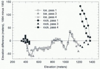
Fig. 10. Bear Lake Glacier. Elevation changes vs map elevation for the three profiles. The “rock” points at high elevations are at the head of the glacier where it is extremely steep (Fig. 9) and the ranger data are prohibitively noisy. Such points are excluded from the error analysis as described in the text.
5. The Problem of Map and Profile Comparison
A. Maps and their quality
In the United States there are two sources of maps showing glacier surface elevations. The first is a set of nine glacier maps made during 1957–58 by the American Geographical Society (1960). They have a scale of 1 : 10000 and a contour interval of 5 m, but few of them have absolute control, which is necessary for comparison with our profiles. The other maps, covering most of Alaska, were made by the U.S. Geological Survey (USGS); they are the maps used here. Many of the USGS maps of interest to us were made from photography acquired in 1949 or the 1950s. Thcy have a scale of 1 : 63360 and a contour interval of 100 ft (30.5 m). The standard of accuracy is half a contour interval (about 15 m) in the vertical, and about 50 m in the horizontal, which is almost two orders of magnitude poorer than the profile data. However, the accuracy of a given map is in fact unknown, and may be better or worse than the standard, depending upon the quality of the aerial photographs used in map construction, the proximity and quality of the ground control, the steepness of the terrain, and other factors. Another problem is that photographs from more than one data have sometimes been used for a single glacier, and contours which are mismatched because of real changes between these dates have been smoothed by the cartographers. Gulkana Glacier, for example, was mapped from a composite of 1954 and 1949 photography. The dates of photography are sometimes incomplete on the maps, and the month when they were taken is generally not given. The exact dates for the glaciers discussed here have been confirmed by the mapping agency.
B. Reference systems
The comparison οf map and profile data requires care in the use of reference systems for both horizontal and vertical coordinates. GPS coordinates are initially calculated in an Earth-centered Cartesian system; these are then transformed to latitude and longitude on the World Geodetic System 1984 (WGS84) ellipsoid, and height above this ellipsoid. The WGS84 ellipsoid and datum, which are essentially equivalent to the North American Datum 1983 (NAD83), are the standard for GPS geodesy in North America. However, most maps in Alaska are referenced to a different system, the North American Datum 1927 (NAD27), so a comparison of profiled and map elevations requires other transformations. First, the profiled latitude and longitude are transformed to the NAD27 reference system, which usually involves a horizontal shift of almost 200 m. Secondly, the NAD27 latitude and longitude are transformed to planar coordinates by a conformal projection to the particular zone of the Universal Transverse Mercator system (UTM) in which a glacier is located. The UTM coordinate grid is marked on the USGS maps, allowing co-registration. Thirdly, the profiled elevations are transformed from heights above the WGS84 ellipsoid to elevations above the geoid (orthometric heights) using the National Geodetic Survey model GEOID94 (Alaska), which gives a best estimate of the separation between the ellipsoid and the geoid throughout Alaska. This model can have errors on the order of 2 m, especially in mountain areas.
All profile coordinates are ultimately measured with respect to the WGS84 coordinates of a benchmark at or near the fixed receiver. The ellipsoidal heights of these benchmarks are often estimated from their tabulated orthometric heights. This means that the ellipsoidal height of the benchmark is not always known accurately, because of errors in the geoid model. For this reason we archive the benchmark coordinates with the rest of the data to permit future corrections, if necessary.
C. Elevation changes
With a common reference system established as just described, the map and the track of the profiled points may be co-registered. The horizontal coordinates of points where the profile (or profiles) intersect the contour lines are then determined using a digitizing table and suitable numerical algorithms. This permits, finally, the comparison of the profiled and map elevations. The errors in registration and in the determination of the intersections are both about 10 m (standard deviation) in the horizontal. The first is more critical because it can lead to systematic errors in elevation, but both errors are small compared with the 50 m horizonial map standard noted above. The elevation error resulting from a horizontal error is the product of this horizontal error and the tangent of the surface slope angle. In regions of steep surface slopes this error can be 10 m or more.
As a test of the accuracy of the maps, we measured apparent elevation changes in unglacierized areas along the profiles. Some of the results are indicated by the solid symbols in Figures 4, 7, and 10. The elevation comparisons on steep rocky passes at the heads of the glaciers are poor, as expected from the above discussion of horizontal errors. Of course, changes in glacierization and seasonal snow cover are also contributing factors. Fortunately, in the high steep regions there is usually little glacier area. The elevation comparisons in the proglacial areas are better, even though the surface is sometimes steep there as well. The results of these proglacial comparisons are shown in (Table 2). In this table, the mean difference is the apparent elevation change averaged over all points where the profiles cross bedrock contours. The standard deviation about this mean indicates the typical Scatter of a contour elevation about this mean difference, and as such is a measure of the random error in the contour lines (about 10 m vertical). The standard deviation of the mean is a measure of how well the mean difference is determined. This standard deviation, when compared to the mean difference itself, shows that the mean difference is not convincingly different from zero for any of the glaciers. This suggests that the elevations on the maps are correct to within at least a few meters, and that no systematic corrections for these glaciers seem to be justified on the basis of this error determination.
Table 2. Profiled minus map elevations in unglacierised region below termini.

The results of this analysis are that in the proglacial areas the systematic errors in map elevations are small, but the contours have random errors of about 10 m. The errors are larger in the highest parts of the glaciers, but this is usually not serious because there is little area there. The main question is whether over the main glacier area the errors are similar to those in the proglacial area. We know that very large errors sometimes occur when the photographs used for map construction have poor detail in snow-covered areas, but we have examined the photographs used for all three glaciers, and find no obvious problems with them. Nevertheless, in the case of Bear Lake Glacier, at least, we suspect that there are errors which exceed those in the proglacial area. Figure 10 shows a trough and peak combination in the elevation change between about 900 and 1100 m, which seems physically unreasonable. It therefore appears that the effect of additional systematic errors such as these needs to be considered.
Strong tectonic activity in south-central Alaska could also contribute to differences in the profiled and map elevations. For example, a great earthquake in 1964 caused subsidence of about a meter in the vicinity of Bear Lake and Worthington Glaciers (Reference Small,, Wharton, and Leipold,Small and Wharton, 1969). No corrections for these effects have been made.
D. Volume change
To calculate the volume change of a glacier, the first step is to define the glacier’s original boundaries on the map. This usually involves some arbitrary decisions regarding what areas to include and whether a basin-wide volume change is to be determined (for hydrologic purposes, for example) or a change limited to connected parts of a glacier. (We present results for the “connected glacier” here.) The next and most critical step is to extrapolate the elevation data from a profile (or profiles) to the glacier surface, thus obtaining an approximate but complete topographic map at the time of profiling. This is done by constructing a “new” contour line (at the time of profiling) from each “old” one (from the map) using the following rules: (1) The new contour has the elevation of the old one plus an amount Δh, the elevation differences, read at the appropriate elevation from Figure 4, 7, or 10. (For the highest contours it is usually necessary to extrapolate to elevations slightly higher than those measured.) (2) The intersection point of the new contour with the valley wall is found by moving the old point up (or down) the valley wall by a vertical amount Δh, along a line drawn between the old intersection points on opposite sides of the valley. (3) The new contour is a contracted version of the old, strained between the old points of intersection with the valley walls to fit between the new. This procedure determines the new boundaries of the glacier and a new set of contour lines at irregularly spaced elevation intervals. A set of contour lines Corresponding to the elevations on the original map (at each 100 ft elevation) is found by interpolation. A variation of this approach is used in the lowest part of the glacier, where a combination of the profiled elevations and extrapolated map contours is used to construct the topography of the deglacierized area. The new position of the terminus can be identified by a sharp kink and flattening in the profile data. For each of the three glaciers this position coincides closely with the position of the terminus as estimated from U2 photographs (obtained during the NASA High Altitude Aerial Photography Program), which were used to fill in the details of the terminus shape at the time of profiling.
With the original and new maps in hand, the last step in the calculation of volume change is a standard one, for which we use the method of Reference Finsterwalder,Finsterwalder (1954). We compute the average thickness change over the glacier by dividing the total volume change by the average of the old and new planimetric areas.
The error in the average thickness changes is difficult to estimate. We believe that there are three dominant contributions to this error: (1) the random contour error of 10 m which was found in the proglacial area, (2) additional, systematic contour errors over the glacier surface as noted above in connection with Bear Lake Glacier, and (3) an error due to limited coverage, because our measurements are along profiles and, thus, do not cover the complete surface. The first of these (10 m divided by the square root of the number of contours used in the volume-change estimate when the weighting is equal) is roughly 2 m. The second and third errors are difficult to quantify, but limited analysis shows them to be about 3.5 and 2 m, respectively. Treating these three contributing errors as independent, the net error in the average thickness change is 4–5 m. Other errors, including that associated with making seasonal corrections (discussed below), also add to the net error, but their contribution is smaller. Combining all these terms gives an estimated net error in the seasonally corrected average thickness changes of roughly 5 m (standard deviation). This net error applies to all three glaciers discussed here.
6. Glacier Changes
Most of the measured surface elevation changes at the points where the profiles cross the map contours are shown for the three glaciers in Figures 4, 7, and 10: the changes are summarized in (Table 3). Most notable is the areal average thickness change between the time of the map photography (typically the early 1950s) and of profiling (1993 and 1994): −10.9, + 11.1, and −7.8 m for Gulkana, Worthington and Bear Lake Glaciers, respectively, each with a 4 or 5 m error. Assuming that the variation of density with depth has not changed significantly, this is the average net mass balance (ice equivalent) between the measurement dates.
Table 3. Glacier changes.
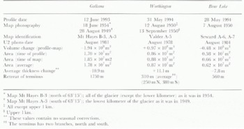
The behavior of the termini is also summarized in (Table 3). All three glaciers retreated during the 40–45 year period between the map photography and the profile measurements. Worthington, with the most positive balance, retreated the least. As noted above, the terminus positions of all three glaciers appear similar at the time of profiling (1993–94) and the time of the U2 photography (typically in the late 1970s and early 1980s). Most of the retreat therefore seems to have occurred between about 1950 and about 1980, although an uncertainty of roughly 200 m in our determination of positions from this photography needs to be kept in mind.
The average thickness changes listed in (Table 3) for Worthington and Bear Lake Glaciers contain a significant seasonal contribution because the profiles were measured during spring, while the map photography was acquired in late summer (late in the ablation season). The thickness changes during the interval late summer 1950-late summer 1993 can be approximated by subtracting the average snow thickness at the time of profiling from the thickness changes in (Table 3). For Bear Lake Glacier we use a value of 4.4 m for the snow thickness, estimated from the 1993–94 winter balance of nearby Wolverine Glacier (preliminary USGS data; personal communication from D. Trabant, 1996). For Worthington Glacier we use the same value, although it is more uncertain because of the greater distance from Wolverine Glacier (Fig. 1). For Gulkana Glacier we make no correction because most of the map photography was acquired in spring. The resulting seasonally corrected average thickness changes are summarized in (Table 4). The uncertainty is 5 m (standard deviation), as discussed above. The thickness change of Worthington Glacier was positive (or perhaps near zero) while the changes of the other two were strongly negative.
Table 4. Seasonally corrected thickness changes.

7. Comparison with Other Measurements: The Regional Picture
Because the main purpose of airborne elevation profiling is to provide information about regional mass-balance patterns, it seems worthwhile, even in this early stage of our program, to consider these patterns using our results and data from other sources when relevant.
The best conventional mass-balance data in central and south-central Alaska are from Gulkana and Wolverine Glaciers (Fig. 1). The measurements began in 1965, and are published in six volumes and bulletins describing the balances of glaciers worldwide (e.g. Reference Haeberli,, Hoelze and Bösch,Haeberli and others, 1994). Limited data from Black Rapids Glacier (Fig. 1) also exist (Reference Heinrichs,, Mayo,, Trabant and March,Heinrichs and others, 1994). In addition, thickness changes of several glaciers in Figure 1 have been estimated for various time periods. In the Alaska Range, Gulkana (Reference Mayo, and Trabant,Mayo and Trabant, 1986), West Gulkana (Reference Marcus, and Reynolds,Marcus and Reynolds, 1988) and East Fork (Reference Clarke,Clarke, 1986) have been investigated. In the Kenai Mountains, Wolverine (Reference Mayo,, Trabant,, MeBeath,, Juday,, Weller and Murray,Mayo and Trabant, 1984; Reference Mayo,, March,, Trabant. and Dwight,Mayo and others 1985) and two in the Bradley Lake basin (Reference Bredthauer,, Harrison, and Bredthauer,Bredthauer and Harrison, 1984) have been measured. The glaciers in the Kenai Mountains are of interest because they are close to Bear Lake Glacier, but the intervals studied are sufficiently different from ours to make useful comparisons difficult. However, it is interesting that several of these glaciers (Wolverine, and Kachemak and Nuka in the Bradley Lake basin) have retreated during intervals of positive or near-zero balance, and thus have shown the same behavior as Worthington Glacier noted above.
A. Gulkana Glacier and the Alaska Range
A history of the surface elevation of Gulkana Glacier from 1875 to 1983 was given by Reference Mayo, and Trabant,Mayo and Trabant (1986). They noted that strong thinning earlier in the century had changed to weak thickening by the mid-1970s, and predicted that any additional recession would amount to at most 100 m. This has proved to be correct, as noted above. Despite the stable terminus position, measurements at three index sites indicate that the trend in balance between the mid-1980s and 1994 has been strongly negative.
Reference Mayo, and Trabant,Mayo and Trabant (1986) argued that the mass balance of Gulkana Glacier was representative of balances in the eastern and central Alaska Range, citing as evidence the common existence of recent, unvegetated, ice-cored moraines throughout the area. We also note that there is a similarity between the annual balance of Gulkana and that of nearby Black Rapids Glacier (Reference Heinrichs,, Mayo,, Trabant and March,Heinrichs and others, 1994, Reference Heinrichs,, Mayo,, Echelmeyer, and Harrison,1996). West Gulkana Glacier (located about 4 km from Gulkana Glacier) decreased in thickness by an average of about 16 m between 1957 and 1986 (Reference Marcus, and Reynolds,Marcus and Reynolds, 1988; Reference Bredthauer,, Harrison, and Bredthauer,Chambers and others, 1991). Our data allow another comparison, this one between Gulkana and East Fork Glaciers. East Fork is a 16 km long glacier in the Susitna basin of the south-central Alaska Range, about 70 km west of Gulkana Glacier (Fig. 1). During the interval 1949–82 the average thickness of East Fork Glacier decreased by about 13 m (Reference Clarke,Clarke, 1986). During the interval covered by our measurements, 1954 (1949 near the terminus) to 1993, Gulkana Glacier thinned by about 11 m. While the time periods are slightly different for the two glaciers, the similarity in the total thinning is probably significant. The errors in all of these measurements are either large or unknown, but taken together they lend support to the claim that Gulkana Glacier has regional representativity. Over how large a region, and for what distribution of glacier area with elevation, are still open questions.
B. Thickness change and behavior of terminus
An attractive method for obtaining a regional picture of mass balance is to try to relate the average change in thickness to the change in terminus position (or the change in thickness there), because the latter is easily mapped. For example, Reference Oerlemans, and Fortuin.Schwitter and Raymond (1993) found that the ratio of the change in thickness at the terminus to the change averaged over the glacier surface lay in a reasonably narrow range (0.1–0.4) for 15 valley glaciers which they examined. They pointed out that the approach is likely to fail for short time intervals or when complex transient effects are important. Worthington Glacier and the glaciers in the Kenai Mountains noted above appear to be examples of this failure, because they have retreated at times of positive or near-zero balance. It is true that most of these balance estimates depend upon reasonable map accuracy, but taken together they suggest that a simple relation between balance and terminus position may not exist for some glaciers, even over time intervals exceeding 40 years.
8. Summary
A relatively lightweight and compact elevation profiling system has been developed for mountain glaciers and has been found to have a typical accuracy of 0.3 m. The system can provide accurate baseline data against which future elevation changes can be measured on a relatively short time-scale. Past changes can be estimated by comparing present elevations with those on existing maps. Such comparisons are limited primarily by the quality of the maps.
Elevation profiles measured during 1993 and 1994 on three glaciers in central and south-central Alaska have been compared with elevations from maps made in the early 1950s. Corrections have been made to account for differences in seasonal timing between the profiles and the photographs used for map construction. Worthington Glacier (in the central Chugach Mountains) experienced an average thickness change of +7 m. This positive or near-zero thickness change contrasts with negative thickness changes experienced by the other two glaciers, −11 m for Gulkana (in the central Alaska Range 240 km north of Worthington) and −12 m for Bear Lake (Kenai Mountains, 220 km southwest of Worthington). The errors in the average thickness changes are about 5 m (standard deviation), and are largely due to errors in the maps. Our estimation of these errors is, in part, obtained by comparison of profiles with map contours in proglacial areas. Other significant contributions to the net error include the limited coverage of the profiles over the glacier, and additional map errors in regions of snow-cover, possibly because of a reduction in photographic surface definition. These latter two errors are somewhat difficult to quantify.
Within the estimated errors, Worthington Glacier has had a positive or near-zero balance during the interval studied, and yet it has retreated. Other glaciers in south-central Alaska have had similar behavior, indicating that changes in glacier length are not necessarily good indicators of glacier mass balance.
Acknowledgements
We are grateful to G. L. Mader for supplying GPS data reduction software, to C. Bakken for help in installing instruments in the aircraft, and to D. Trabant for obtaining map information. We also thank R. LeB. Hooke, T. Scambos, and D. Trabant for their many helpful comments on a previous version of the manuscript. The GPS receivers were manufactured by Trimble; the laser altimeter by IBEO. Financial support is from the National Aeronautics and Space Administration, grant NAGW 3727. The initial development of the system was supported by the National Oceanic and Atmospheric Administration, Office of Global Programs.


