


Introduction
Atmospheric warming and changes to oceanic conditions over the latter half of the 20th century and beginning of the 21st century have resulted in accelerated recession and mass loss from glaciers and ice shelves around the Antarctic Peninsula (Cook and others, Reference Cook2016; Hogg and others, Reference Hogg2017; Fieber and others, Reference Fieber2018). Changes include the rapid disintegration of several ice shelves, including Larsen A (Rott and others, Reference Rott, Skvarca and Nagler1996), Prince Gustav (Cooper and others, Reference Cooper1997) and Larsen B (Rack and Rott, Reference Rack and Rott2004), and the enhanced recession of Wilkins (Braun and others, Reference Braun, Humbert and Moll2009) and Larsen C (Hogg and Gudmundsson, Reference Hogg and Gudmundsson2017). The timing of ice-shelf disintegration events coincides with the northern migration of the −9°C mean annual isotherm (Morris and Vaughan, Reference Morris, Vaughan, Domack, Levente, Burnet, Bindschadler, Convey and Kirby2003), a lengthening of the melt season (Barrand and others, Reference Barrand2013) and where positive degree days exceed 200 d a−1 (Fyke and others, Reference Fyke, Carter, Mackintosh, Weaver and Meissner2010). Furthermore, recent research (e.g. Pritchard and others, Reference Pritchard2012; Paolo and others, Reference Paolo, Fricker and Padman2015; Adusumilli and others, Reference Adusumilli2018) has illustrated the significance of basal melting on ice-shelf mass balance, related to changes in oceanic conditions (e.g. Robertson and others, Reference Robertson, Visbeck, Gordon and Fahrbach2002; Meredith and King, Reference Meredith and King2005; Padman and others, Reference Padman2012) and sea-ice concentrations (Stammerjohn and others, Reference Stammerjohn, Martinson, Smith and Iannuzzi2008; Massom and others, Reference Massom2018).
As well as atmospheric and ocean-driven thinning, further conditioning factors that enhance ice-front recession include: (i) a concave ice-front geometry from an ice shelf's lateral pinning points (e.g. Doake and others, Reference Doake, Corr, Rott, Skvarca and Young1998); (ii) an increase in flow speed in years preceding disintegration (e.g. Rack and others, Reference Rack, Doake, Rott, Siegel and Skvarca2000; Rack and Rott, Reference Rack and Rott2004); (iii) the presence of pinning points such as ice rises (e.g. Hughes, Reference Hughes1983; Braun and others, Reference Braun, Humbert and Moll2009); (iv) structural (in)stability along suture zones (e.g. Glasser and Scambos, Reference Glasser and Scambos2008; Kulessa and others, Reference Kulessa, Jansen, Luckman, King and Sammonds2014) and at the calving front (e.g. Braun and others, Reference Braun, Humbert and Moll2009; Holt and others, Reference Holt, Glasser, Quincey and Siegfried2013); and (v) the presence of either surface meltwater (e.g. Scambos and others, Reference Scambos, Hulbe, Fahnestock, Domack, Levente, Burnet, Bindschadler, Convey and Kirby2003) or infiltrated brine within the ice shelf (Scambos and others, Reference Scambos2009). A combination of these conditioning factors can lead to major calving events through hydrofracture (Scambos and others, Reference Scambos, Hulbe, Fahnestock and Bohlander2000, Reference Scambos, Hulbe, Fahnestock, Domack, Levente, Burnet, Bindschadler, Convey and Kirby2003; MacAyeal and others, Reference MacAyeal, Scambos, Hulbe and Fahnestock2003; Banwell and others, Reference Banwell, MacAyeal and Sergienko2013, Reference Banwell, Willis, Macdonald, Goodsell and MacAyeal2019) or plate-bending initiated by differential stresses at the ice front (Scambos and others, Reference Scambos2009). Regardless of the final processes involved, the removal of buttressing ice has been shown to alter the dynamics of grounded ice, increasing tributary glacier flow speed, and resulting in greater discharge of fresh, meteoric ice into the Southern Ocean (Rott and others, Reference Rott, Rack, Skvarca and Angelis2002, Reference Rott, Rack and Nagler2007, Reference Rott2018; Hulbe and others, Reference Hulbe, Scambos, Youngberg and Lamb2008; Berthier and others, Reference Berthier, Scambos and Shuman2012; Fürst and others, Reference Fürst2016; Friedl and others, Reference Friedl, Seehaus, Wendt, Braun and Höppner2018).
Mercer (Reference Mercer1978) and Vieli and others (Reference Vieli, Payne, Shepherd and Du2007) noted that glaciological changes (e.g. ice-front morphology and evolution, glacier structures and ice-shelf dynamics) occur well in advance of enhanced recession and breakup of ice shelves. This led Glasser and Scambos (Reference Glasser and Scambos2008), Glasser and others (Reference Glasser2009, Reference Glasser2011), Braun and others (Reference Braun, Humbert and Moll2009) and Holt and others (Reference Holt, Glasser, Quincey and Siegfried2013, Reference Holt2014) to examine an extensive back-catalogue of satellite imagery to investigate the glaciological conditions of Antarctic Peninsula ice shelves. Their work collectively illustrated the requirement for monitoring glaciological factors to identify precursors to ice-shelf disintegration and assess the impacts of environmental change on ice-shelf systems.
The aim of this study is to investigate recent glaciological changes to three ice shelves on the southwest Antarctic Peninsula: Bach, Stange and George VI (Fig. 1). Changes to George VI and Stange ice shelves were described by Holt and others (Reference Holt, Glasser, Quincey and Siegfried2013) and Holt and others (Reference Holt2014) respectively, but now a further decade's worth of satellite imagery has been acquired, offering higher quality and finer-resolution data to assess more recent developments. A combination of Landsat 7 ETM+, Landsat 8 OLI and Sentinel 2 satellite scenes, supported by ASTER imagery, is used to measure decadal areal changes at the ice fronts, examine structural and surface feature evolution, and calculate ice-shelf flow speed from 2009/10 to 2019/20.

Fig. 1. (a) Location of Bach, Stange and George VI ice shelves on the Antarctic Peninsula. Red dot between Cryosat Ice Stream (IS) and Grace IS is the location of the Gomez ice core as mentioned in the text. The location of the ice divide on George VI Ice Shelf illustrates the divergence of flow towards the northern and southern region. GT, George VI Tributary; ST, Stange Tributary. (b) MEaSUREs surface velocity (Rignot and others, Reference Rignot, Mouginot and Scheuchl2011). (c) BedmapV2 ice thickness (Fretwell and others, Reference Fretwell2013). (d) Extent of panels (a–c) in the wider context of Antarctica.
Southwest Antarctic Peninsula ice shelves
Atmospheric temperature reconstructions from the Gomez δ18O ice core record (Thomas and other, Reference Thomas, Marshall and McConnell2008) (location in Fig. 1a) show a warming trend in the southwest Antarctic Peninsula since the 1900s, and by ~2.7°C since the 1950s (Thomas and others, Reference Thomas, Dennis, Bracegirdle and Franzke2009) despite short-lived periods of atmospheric cooling on the peninsula in the mid-to-late 1990s and 2015/16 (Picard and others, Reference Picard, Fily and Gallee2007; Turner and others, Reference Turner2016; Banwell and others, Reference Banwell2021). In 2003, the seemingly critical −9°C mean annual isotherm stretched across Alexander Island into George VI Sound, before heading north towards Larsen C (Morris and Vaughan, Reference Morris, Vaughan, Domack, Levente, Burnet, Bindschadler, Convey and Kirby2003). Simultaneously, the upper ocean on the western Antarctic Peninsula underwent warming in the second half of the 20th century (Meredith and King, Reference Meredith and King2005), with Martinson (Reference Martinson2012) and Schmidtko and others (Reference Schmidtko, Heywood, Thompson and Aoki2014) reporting an increase in the delivery of warmer and saline circumpolar deep water (CDW) onto the continental shelf, heading landward through glacial canyons (Meredith and others, Reference Meredith2017). Over longer timescales, sea-ice extent has shown a strong negative trend on the west Antarctic Peninsula, with a moderate trend for earlier retreat in spring, and a more pronounced trend towards a later advance in autumn (Stammerjohn and others, Reference Stammerjohn, Martinson, Smith and Iannuzzi2008). There are, however, temporal variations with observations showing summer sea ice disappearing almost completely in 15 of the 20 years since 2000 in Ronne Entrance (sea ice remaining only in 2006, 2007, 2016, 2017 and 2020) (NSIDC Sea Ice Index, 2020).
Within the southwest Antarctic Peninsula region are four ice shelves – George VI, Stange, Bach and Wilkins – covering a total area of ~49 000 km2, with their drainage basins totalling ~161 000 km2 (Rignot and others, Reference Rignot, Mouginot and Scheuchl2011). George VI, Stange and Bach are considered in more detail below with key attributes summarised in Table 1. Wilkins Ice Shelf is not investigated here because there are few glaciological changes observed in a preliminary study using Landsat 8 OLI imagery acquired between 2013 and 2019, and because it has recently been described elsewhere (e.g. Rankl and others, Reference Rankl, Fürst, Humbert and Braun2017).
Table 1. Key attributes of George VI Ice Shelf, Stange Ice Shelf and Bach Ice Shelf

Sources noted in final column.
Bach Ice Shelf
Bach Ice Shelf occupies the southern region of Alexander Island (Fig. 1a). It comprises four main flow units with a confluence near the ice front, the most dominant being Weber and Boccherini inlets. It has a spatially averaged surface flow speed of 62 m a−1, with a maximum speed of ~230 m a−1 recorded at the grounding zone of Lovell Glacier (Fig. 1b). At the ice front, flow speeds reach a maximum of ~140 m a−1. Between 1947 and 2008, ~311 km2 of ice was lost from its front (Cook and Vaughan, Reference Cook and Vaughan2010), but it maintained its sinusoidal-shaped ice-front geometry and covered an area of ~4536 km2 in 2010 (Holt, Reference Holt2012).
Holt (Reference Holt2012) noted extensive melt pools that fill structurally-influenced channels in the northern reaches of Weber, Boccherini and Williams inlets, and isolated pools also occur in the northern section of Stravinsky Inlet. Ice dolines in the northern extents of Boccherini and Williams inlets suggest a hydrological link between the surface and an englacial environment. Bach Ice Shelf has a mean firn thickness of ~14.6 m (van den Broeke, Reference van den Broeke2005). Holt (Reference Holt2012) also observed the development of two fracture units between October and December 2004, which at the time were ~9 km from the ice front.
Stange Ice Shelf
Stange Ice Shelf is the most southern and westerly ice shelf on the Antarctic Peninsula (Fig. 1a). It measured ~7900 km2 in 2011 (Holt and others, Reference Holt2014), and displayed a complex dynamic configuration owing to several glacial basins on the English Coast, Spaatz Island and Smyley Island from which tributary glaciers flow. It has three independent ice fronts, the largest (Stange North) of which calves into Ronne Entrance. Two smaller ice fronts (Stange Central and Stange South) calve into Carroll Inlet; an isolated embayment that is typically filled with fast ice. The mean flow speed for Stange Ice Shelf is ~200 m a−1: The most southerly ice front is the most dynamic, fed by Landsat Ice Stream that reaches the speeds of ~800 m a−1 (Rignot and others, Reference Rignot, Mouginot and Scheuchl2011) (Fig. 1b). It was here that Holt and others (Reference Holt2014) noted the greatest structural and dynamic changes between 2001 and 2011 including the increased presence of shear-induced fracturing between flow units.
Holt and others (Reference Holt2014) attributed surface elevation changes (inferred ice-shelf thinning) to an increase in basal melting, as also noted on the nearby George VI and Wilkins ice shelves (Padman and others, Reference Padman2012; Holland and others, Reference Holland, Jenkins and Holland2010), though some lowering may also result from firn compaction at its northern front. Stange Ice Shelf sits between the −11 and −15°C mean annual isotherms (Morris and Vaughan, Reference Morris, Vaughan, Domack, Levente, Burnet, Bindschadler, Convey and Kirby2003) and for much of its surface area, the mean number of melt days (2006–2012) was ~35 d a−1, ranging from ~80 d a−1 at its northern ice front and only 10 d a−1 along the English coast (Holt and others, Reference Holt2014). Key attributes are presented in Table 1.
George VI Ice Shelf
George VI Ice Shelf is the second largest remaining on the Antarctic Peninsula covering an area of ~23 000 km2. It has two frontal margins situated ~450 km apart: a northern ice front (George VI North) that calves into Marguerite Bay, with three further ice fronts located in its southern region (George VI South). The ice shelf is fed predominantly from glaciers draining Palmer Land that flow across George VI Sound and butt against Alexander Island. Occasionally these large glaciers run into smaller tributaries flowing in the opposite direction from Alexander Island, but for only a few kilometres. The glaciers from Palmer Land reach the speeds of up to 700 m a−1 in the northern region and are interspersed with less active areas of ice moving at the speeds of just 10s m a−1 (Fig. 1b). At approximately −68°8′0″ W −72°32′0″ S, there is an ice-shelf divide (see Fig. 1a): Tributaries entering George VI Sound south of this flow ~150 km towards George VI South at speeds of ~300–400 m a−1. Tributary glaciers GT02 to Grace Ice Stream feed the ice front located between Monteverdi Peninsula and the Eklund Islands. Further southwest, tributary glaciers GT05 to Sentinel Ice Stream feed an ice front between the Eklund Islands and DeAtley Island, with a smaller ice front fed by glaciers GT08 and GT09. These three southern fronts are dynamically independent but do form a continuous ice-shelf system in the southern region.
Widespread recession of George VI's ice fronts has been previously reported, including a loss of ~1255 km2 between 1974 and 2010 from George VI North (Holt and others, Reference Holt, Glasser, Quincey and Siegfried2013) and a loss of ~1400 km2 between 1947 and 2008 at George VI South (Cook and Vaughan, Reference Cook and Vaughan2010). At the southern margin, ice entering the shelf from GT05, GT06 and Sentinel Ice Stream saw a considerable increase in the speed of up to 340±38 m a1 from 1989 to 2010 owing to the removal of the stabilising ice front and associated ice-shelf thinning (Holt and others, Reference Holt, Glasser, Quincey and Siegfried2013; Hogg and others, Reference Hogg2017).
Surface melting occurs regularly along its northern extent in the austral summer, with melt pools and interconnected channels forming in structurally-influenced longitudinal and transverse troughs (Reynolds and Hambrey, Reference Reynolds and Hambrey1988; Holt and others, Reference Holt, Glasser, Quincey and Siegfried2013; Banwell and others, Reference Banwell2021; Barnes and others, Reference Barnes2021). George VI Ice Shelf is also known to have a high basal melt rate driven by the flooding of CDW into the ice-shelf cavity (e.g. Holland and others, Reference Holland, Jenkins and Holland2010; Fricker and Padman, Reference Fricker and Padman2012; Adusumilli and others, Reference Adusumilli2018). Key attributes are summarised in Table 1. Further, numerical modelling illustrates the importance of George VI Ice Shelf to future sea level rise, with Schannwell and others (Reference Schannwell, Barrand and Radić2016) projecting that up to 70% of the total contribution from the Antarctic Peninsula's ice-shelf tributary glaciers comes from George VI Ice Shelf alone.
Data and methods
Landsat 7 ETM+ (2005–2010), Landsat 8 OLI (2013–2020), Sentinel 2 (2016–2020) and ASTER (1999–2010) scenes were used in this study (online Supplementary Table S1). Optical images were downloaded from the USGS's Earth Explorer collection (Level 1C) via the Semi-Automatic Classification plug-in (SCP; Congedo, Reference Congedo2016) in QGIS 3.4. All Landsat and Sentinel 2 scenes were atmospherically corrected using a dark object subtraction method, with Landsat bands 2, 3 and 4 also pan-sharpened to 15 m pixel resolution using a Brovey conversion in the SCP. The single ASTER scene was only used for additional visual analysis and was not pre-processed to the same level as other data.
Ice-front positions were manually mapped to an accuracy of ±2 pixels in ArcGIS 10.7 at a scale of 1: 50 000 for seven austral summers between 2009 and 2020 (2009/10, 2013/14, 2014/15, 2016/17, 2017/18, 2018/19, 2019/20), taking advantage of the finest available Landsat (15 m pixel−1) and Sentinel 2 (10 m pixel−1) visible bands. Ice-shelf areal loss and gain were calculated between each austral summer studied, and for the full observation period. Uncertainty analysis was conducted on Bach Ice Shelf, whereby its frontal position and subsequent area change was mapped three times for each year. This analysis revealed that uncertainty in area change was at most ±0.5 km2 – a fraction of the ice-shelf area change recorded between time periods.
Structural assessment for all three ice shelves was conducted for the austral summers 2009/10, 2013/14 and 2019/20 using cloud-free Landsat ETM+, Landsat OLI and Sentinel 2 scenes; visual analysis of intervening years suggested only minor changes had occurred, so we opted to quantify changes over a 4–6 year timescale. Additional analysis of Bach Ice Shelf was undertaken using Landsat ETM+ and ASTER imagery acquired between 2001 and 2005 to show the development of two distinctly large fractures first noted by Holt (Reference Holt2012). Our quantitative structural analysis focused on the lengths and widths of open fractures on Bach, Stange and George VI. We define ‘open fractures’ as those that have a clear, sharp boundary between the fracture edge and the surrounding ice shelf for all or part of its length. If the chasm was sufficiently wide, smooth sea ice, a melange of calved blocks and sea ice, or open water was visible within the fracture. We first measured open fracture length from tip to tip along its centreline, then measured the widest part of the open fracture orthogonal to the centreline. We did not quantify fractures that were infilled with snow, or considered to be the surface expression of basal crevasses due to difficulties in measuring their width. These ‘smooth’ fractures are no less important and were instead considered in a qualitative analysis as part of the wider discussion.
We calculated flow fields for 2019/20 using a Fourier-based ‘co-registration of optically sensed images and correlation’ approach (COSI-Corr; Leprince and others, Reference Leprince, Barbot, Ayoub and Avouac2007). COSI-Corr is an add-in for ENVI Classic (available as part of the ENVI 5.5 package), which was developed for use in geosciences. It allows retrieval of sub-pixel displacements between good quality optical images and is one of the most robust methods for calculating glacier flow (Heid and Kääb, Reference Heid and Kääb2012). Flow speeds were calculated for all of Bach and Stange ice shelves, whereas for George VI Ice Shelf only the two frontal regions were considered as prior investigations (e.g. Holt and others, Reference Holt, Glasser, Quincey and Siegfried2013) illustrated that structural and dynamic changes were focused in these areas only. For each ice shelf, we selected near cloud-free Landsat 8 scenes from February 2019 as the t0 image, and a second Landsat 8 scene from October to December 2019 or January 2020 as our t1 image. We used scenes from the same path and row for t0 and t1 to reduce geometric uncertainty in our results. For each image pair, a range of initial (pixel displacement) and final window (sub-pixel displacement) sizes were chosen, guided by expected displacement between images, with the smoothest (i.e. containing less noise) flow field output chosen. Input parameters and flow field output information are shown in Table 2. We then converted displacement from m t0−t1−1 to m a−1. Given the nature of the terrain under investigation, there was limited opportunity to calculate absolute error from regions of stable bare ground, as is common practice with such feature tracking approaches. Instead, we estimate uncertainty of our flow speed calculations to be no more than 1 pixel (15 m t0−t1−1) given the retrieval of sub-pixel displacements via the COSI-Corr method, and relatively flat terrain of an ice-shelf surface that is void of large topographic variations that can introduce substantial errors. We are confident that our uncertainties (metres) are far lower than calculated flow speeds for each ice shelf (tens to hundreds of metres).
Table 2. Key input parameters for COSI-Corr feature tracking processes and resulting pixel resolution

The initial search window calculates pixel displacement, with the final search window used to look for sub-pixel displacements. Step size determines the step (in pixels) that each window will move in an x and y direction during correlation. George VI (South 1) represents the location between Monteverdi Peninsula and the Eklund Islands. George VI (South 2) represents the location between the Eklund Islands and DeAtley Island. Both locations are covered by different Landsat footprints (path/row).
Results
Ice-shelf areal loss and gain
All three ice shelves recorded areal loss from 2009/10 and 2019/20 (Table 3). Spatial (Fig. 2) and temporal (Fig. 3) patterns varied considerably. Bach Ice Shelf underwent sustained recession along its ice front in each of the time periods, with a total of 120.6 km2 ice lost at a net rate of −11.8 km2 a−1. Its frontal geometry became increasingly concave as it decoupled from its Monteverdi Peninsula pinning point in the east. Stange North recorded a total loss of 156.1 km2 between 2009/10 and 2019/20 at a rate of −36.6 km a−1, though −109.9 km2 of this was lost between 2009/10 and 2013/14 alone. Stange Central and Stange South recorded little overall change (−3.6 and −0.4 km2 respectively).

Fig. 2. Ice-front changes observed between 2009/10 and 2019/20. Earliest recorded ice-front position in the satellite era is shown for comparative purposes (1973/74, taken from Holt, Reference Holt2012). (a) Bach Ice Shelf; note the ‘sinusoidal’ shape to its ice-front geometry that becomes less distinct with time. (b) Stange North; note the prominent area that juts out in the centre of the ice front. (c) Stange Central and Stange South. (d) George VI South. (e) George VI North. (f) Extent indicators of panels (a–e).

Fig. 3. Proportional area gain and loss (left-hand axis) and net change (right-hand axis) for each ice shelf (and ice front) in the six time periods observed in this study. Each column = 100% total. (a) Bach Ice Shelf (BIS); note persistent areal loss with only minor gain noted in four of the six periods. (b) Stange Ice Shelf (SIS); note greater loss in the first three periods than the last three. (c) George VI Ice Shelf (GVI); note (i) GVI South recorded loss in the first three time periods, followed by three periods of gain, (ii) GVI North recorded slight increases in four of the six periods, with net loss recorded in 09/10–13/14 and 18/19–19/20 only.
Table 3. Areal gain and loss for each ice front and total ice-shelf area for the six time periods studied

Final column gives total change from 2009/10 to 2019/20.
George VI North saw sustained advance over much of its length, with loss only recorded at its western margin where a sizable polynya was observed in each of the measurement periods. In total, George VI North saw a net gain of 16.7 km2 from 2009/10 to 2019/20. George VI South recorded the largest net change (−497.2 km2) between 2009/10 and 2019/20, but again most of this loss occurred between 2009/10 and 2013/14, concentrated between Monteverdi Peninsula and the Eklund Islands. In 2016/17, 2017/18 and 2019/20, George VI South recorded net gains of +5.1, +44.4 and +16.7 km2 respectively (Table 3). In total, the three ice shelves had a net change of −797.5 km2 from 2009/10 to 2019/20.
Ice-shelf flow speed
Bach Ice Shelf's flow regime is dominated by glaciers entering and flowing through Boccherini Inlet to the ice front (Fig. 4a). Flow speeds in its central portion reached ~150 m a−1 during 2019/20, ~40 m a−1 faster than reported in the MEaSUREs velocity data (hereafter referred to as ‘ca. 2008’; taken from Rignot and others, Reference Rignot, Mouginot and Scheuchl2011) (Fig. 5a).
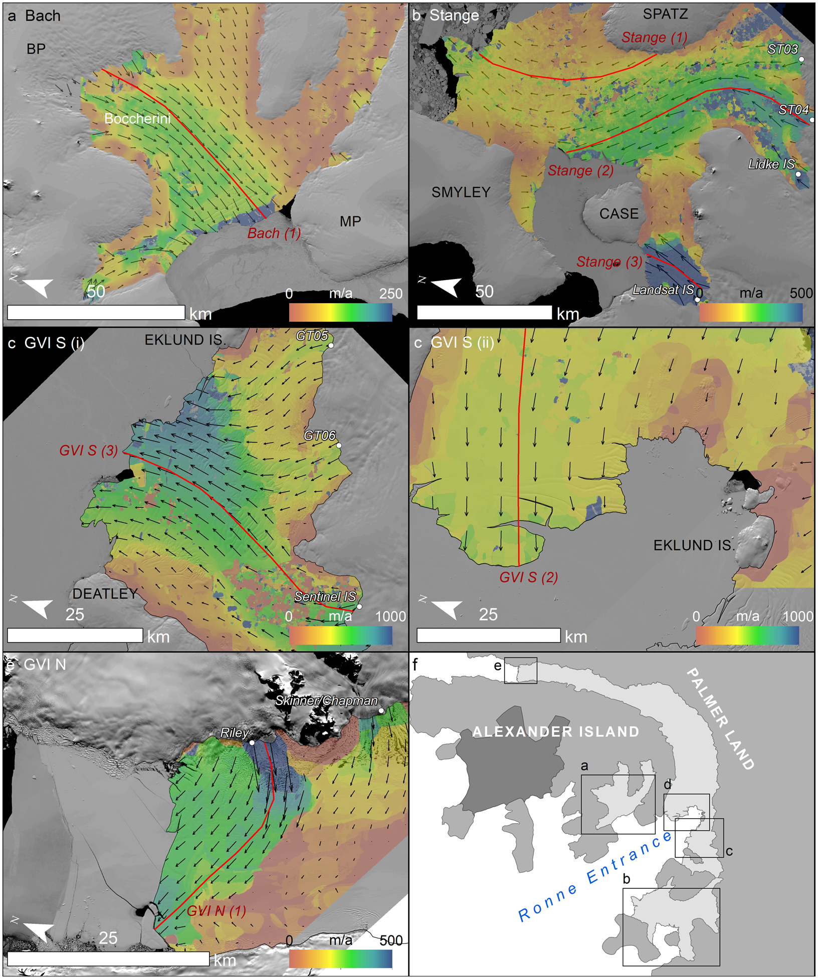
Fig. 4. 2019/20 flow speeds calculated using optical image feature tracking (see Table 2 for parameters). (a) Bach. (b) Stange. (c) George VI South (Eklund Islands to DeAtley Island). (d) George VI South (Monteverdi Peninsula to Eklund Islands). (e) George VI North. Red lines are transects shown in Figure 5. (f) Extent indicators of panels (a–e). Note that the colour ramp scale differs in each panel.

Fig. 5. Flow speeds for 2019/20 (solid lines) and ca. 2008 (MEaSUREs; Rignot and others, Reference Rignot, Mouginot and Scheuchl2011; dashed lines) for transects shown in Figure 4. Note y-axis has different scales in each panel. (a) Increase in flow speeds in the central portion of Bach Ice Shelf. (b) Decrease in flow speeds along Stange (3; Stange South), with little change noted along Stange (1) and Stange (2). Note region of poor image correlation between images from 1 to 20 km for Stange (2). (c) Increase in flow speed along GVI S (3) from 27 km, and GVI N (1) between 0–10 km and 22–26 km. Note region of poor correlation between images from 6 to 18 km for GVI S (3).
Stange Ice Shelf has a complex flow regime, with tributaries entering the ice shelf from catchments on Smyley Island, Spaatz Island and the English Coast, the latter of which has the greatest contribution. Stange North is fed by ice flowing from all three catchments, Stange Central is fed by tributaries from Smyley and the English Coast, and Stange South is fed only by ice flowing from the English Coast. Tributaries ST03, ST04 and the Lidke Ice Stream (Fig. 4b) are responsible for the fastest flow in the main portion of the ice shelf (~450 m a−1). The fastest flow speeds on the ice shelf are found in the Landsat Ice Stream (~750 m a−1) that feeds Stange South. There is little observed change in flow speeds across the main portion of Stange Ice Shelf between ca. 2008 and 2019/20 (Fig. 5b), but speeds on Landsat Ice Stream have decreased by ~120 m a−1.
The calving front of George VI North is dominated by flow from Riley Glacier (Fig. 4e). At its grounding zone, flow speeds measure ~600 m a−1, decreasing to ~300 m a−1 at the calving front over a straight-line distance of ~20 km. Further downstream (~25 km from the ice front), Skinner and Chapman glaciers converge on Palmer Land and enter the ice shelf as one flow unit at the speeds of ~500 m a−1, slowing to ~150 m a−1 within ~10 km. Speeds decrease further towards Alexander Island, reaching only a few tens of m a−1. We observe an increase in flow speed along the centreline of Riley Glacier from ca. 2008 to 2019/20 (Fig. 5c), ranging from +100 m a−1 near the grounding zone (from 0 to 10 km along the transect) to +40 m a−1 between 10 and 23 km along the transect. At its ice front, flow speeds have increased by ~50 m a−1 since ca. 2008.
The southern portion of George VI Ice Shelf is controlled by glaciers entering from the English Coast. Between the Eklund Islands and DeAtley Island, GT05, GT06 and the Sentinel Ice Stream feed the most dynamic part of the ice shelf. Here, at the centre of its calving front, flow speeds reach ~900 m a−1. Speeds along the centreline of Sentinel Ice Stream increased by ~80 m a−1 since ca. 2008 (Fig. 5c). Between Monteverdi Peninsula and the Eklund Islands, flow ranges from <100 m a−1 around the numerous ice rises and ice rumples, to ~420 m a−1 at the centre of the ice front. Ice here is derived from glaciers that enter the shelf about 150 km further upstream (see Fig. 1b for wider perspective). There is little change in flow speed observed between ca. 2008 and 2019/20 in this location (Fig. 5c).
Ice-shelf surface structural assessment
Open fracture lengths and widths were measured for each ice shelf for the austral summers of 2009/10, 2013/14 and 2019/20 (Figs 6–8; Table 4). Few open fractures were observed on Bach Ice Shelf in the three periods, yet the area immediately behind the ice front is dominated by two long fracture sets. Further analysis revealed that these became visible at the surface between October and December 2004 (Figs 7a–f). Since 2004, both fracture sets have increased in length and width as they moved towards the receding ice front. The most northly of these (furthest from the ice front) saw the greatest increase in width from ~85 m in 2009/10 to ~350 m in 2019/20, at which point they both measured >21 km in length. In recent imagery, the opening of the widest fracture displays a smooth surface with no evidence of liquid water or calved blocks at 10 m pixel resolution. Other open fractures on Bach Ice Shelf are transient in nature, cutting back into the shelf from the calving front for a maximum of 3 km in length and 350 m in width.

Fig. 6. Open fracture lengths and widths for Stange (a and b) and George VI (c and d). Note different scales on primary y-axis. Bach Ice Shelf not represented here owing to low numbers of open fractures identified. The lines represent the cumulative frequency of fracture lengths and widths and help illustrate the size distribution and change in size distribution through time. See Table 4 for further statistics. See Figures 7 and 8 for spatial analysis.
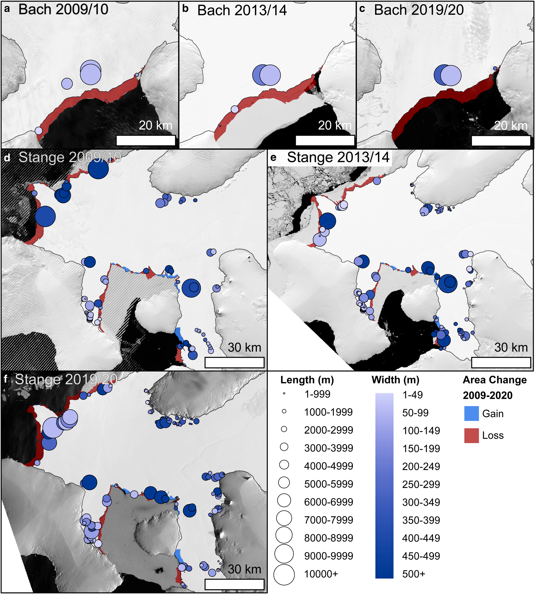
Fig. 7. Spatial distribution of open fractures for 2009/10, 2013/14 and 2019/20 for Bach (a–c) and Stange (d–f). Fracture lengths and widths categorised using histogram bins (see Fig. 6). Fracture length is represented by circle size and fracture width is represented by colour ramp, with darker blue illustrating wider fractures. Circle location represents the fracture's centre point. Area change (gains and losses) also shown.
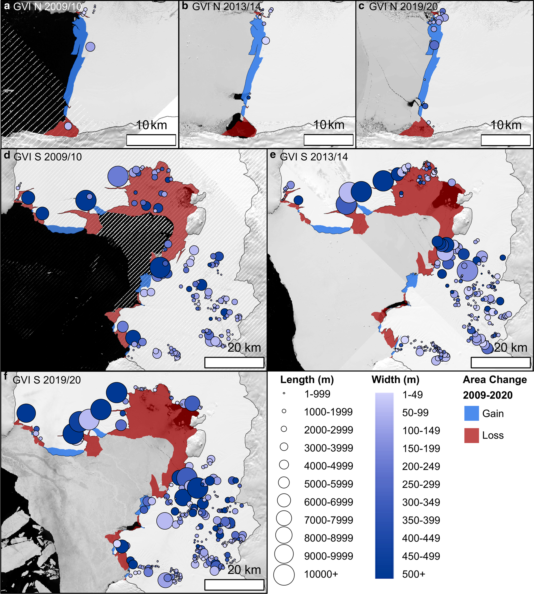
Fig. 8. Spatial distribution of open fractures for 2009/10, 2013/14 and 2019/20 for George VI North (a–c) and George VI South (d–f). Fracture lengths and widths categorised using histogram bins (see Fig. 6). Fracture length is represented by circle size and fracture width is represented by colour ramp, with darker colours illustrating wider fractures. Circle location represents the fracture's centre point. Area change (gains and losses) also shown.
Table 4. Open fracture statistics for Bach, Stange and George VI ice shelves

The number of open fractures increased on Stange Ice Shelf in each of the measurement periods. Of note is a rise in open fracture lengths measuring 500–999 m and +5000 m, and a particularly noticeable increase in fracture widths measuring 100–199 m and 250–299 m (Figs 6a–b). There was a small decrease in the frequency of open fracture widths measuring +500 m in both 2013/14 and again in 2019/20. Cumulative frequency curves (Figs 6a–b) show a greater proportion of open fractures measuring <1999 m in length in 2019/20 than both 2013/14 and 2009/10, but a greater proportion of fracture widths measuring more than 149 m in 2019/20. Wider open fractures were measured at the grounding zone of Spaatz Island and at the southern edge of Stange Central (Figs 7d–f).
A greater number of open fractures were also measured along Stange North (Figs 7d–f) with clustering around the prominent ice-front portion that juts out into Ronne Entrance. The southern region of Stange Ice Shelf saw a reduction in open fractures at both its calving front and in the area occupied by shear-induced fractures in 2010 (see Holt and others, Reference Holt2014). Of those fractures sufficiently wide to see inside their chasms, all are filled by either smooth ice or melange; no areas of open water were observed unless the open fractures were positioned at an ice front.
At George VI North, open fractures were clustered at its eastern pinning point, with individual features observed infrequently along the rest of its calving front. Within this cluster, the fractures became increasingly long and wide throughout the measurement periods (Figs 8a–c). Liquid water, small, calved blocks and smooth ice were observed in open fractures wide enough to see the base of their chasms.
Fractures are widespread across the southern region of George VI Ice Shelf (Figs 8d–f) and are particularly chaotic in places, often containing calved toppled and tabular icebergs, melange, and some pockets of open water, even near the grounding zone. Between Monteverdi Peninsula and the Eklund Islands, the number of open fractures increased from 35 to 61 between 2009/10 and 2013/14, before decreasing to 32 by 2019/20. In 2013/14, clusters of small open fractures were observed lee-side of the Eklund Island ice rumples and account for the observed decrease in the mean fracture length (from 3074 m in 2009/10 to 2198 m) and fracture width (from 422 to 234 m). By 2019/20, a succession of open fractures with wide chasms was observed stemming from the most northerly Eklund Island ice rumple. These features formed a distinctly jagged ice front. The mean open fracture lengths and widths in 2019/20 were 4220 and 289 m, respectively.
Between the Eklund Islands and DeAtley Island, the number of open fractures increased from 112 (2009/10) to 198 (2013/14) to 205 (2019/20). Mean open fracture lengths (2095, 1702, 2093 m respectively) and widths (323, 186, 217 m respectively) were relatively consistent, though a cluster of open fractures west of the largest of the Eklund Islands noticeably increased in length and width between 2009/10 and 2019/20 (Figs 8d–f). In the widest of fractures, smooth sea ice and rough ice melange were observed.
Figures 6c–d illustrate open fracture length and widths for all of George VI Ice Shelf as discussed above, confirming that ~90% of open fractures were <3999 m in length and 80% <199 m in width.
Interpretation and discussion
Bach Ice Shelf
Of the three ice shelves studied, only the front of Bach showed net loss in each of the six time periods. Subtle and discrete episodes of calving were observed along transient fractures at the ice front. Frontal recession led to localised decoupling of the ice shelf from its Monteverdi Peninsula pinning point in the mid-to-late 2000s, and left the front occupying a wider channel than at any other time in the satellite era.
Our analysis indicates widespread acceleration of ice flowing through Boccherini Inlet between ca. 2008 and 2019/20 (Fig. 5). We propose that ice-front recession, and particularly the decoupling from Monteverdi Peninsula, enabled flow to speed up, enhancing longitudinal tensile stresses, which may also explain the rapid appearance of the two fractures in 2004 and their subsequent expansion (Figs 9a–d)

Fig. 9. Features of interest for Bach (a–f) and Stange (g–l) ice shelves as discussed in the sections ‘Bach Ice Shelf’ and section ‘Stange Ice Shelf’, respectively. Figures (a–f) illustrate the development and propagation of two large fractures on Bach Ice Shelf. MP = Monteverdi Peninsula. Panels (g) and (h) show fracture development in the centre of Stange North around the prominent area that juts out into Ronne Entrance. Panels (i) and (j) compare extensive and less extensive (thinner) sea ice in Carroll Inlet adjacent to Stange Central. Note the polynyas and possible plume that exit (sub) surface channels – which are thought to represent the surface expression of basal channels in the ice shelf. Panels (k) and (l) illustrate the closing of shear fractures and migration towards the centre of the Stange South. The solid lines in (k) and (l) represent approximate length of shear zone in 2013–14 and 2019–20. The dashed line in (l) represents the shear fracture distribution shown in (k) for comparative purposes only. RP, Rydberg Peninsula.
Doake and others (Reference Doake, Corr, Rott, Skvarca and Young1998), who investigated the role of a convex calving front in ice-shelf stability following the disintegration of Larsen A Ice Shelf in 1995 and enhanced calving of Larsen B in 1996, illustrated that a convex ice front provided a ‘compressive arch’, that once removed, permitted enhanced calving. Since 1973, Bach's ice front became increasingly concave along its length (Fig. 2a). Two large fracture sets developed in 2004 and gradually increased in length and width as they migrated towards the receding ice front. Owing to their geometry, calving along these fractures would undoubtedly remove the last remaining convex portion from the calving front, leaving a concave geometry across its length that may lead to further instabilities.
Stange Ice Shelf
Despite a net loss of 156.1 km2 between 2009/10 and 2019/20, Stange North's ice front maintained its distinct convex ice-front geometry. However, the prominent area that juts out into Ronne Entrance reduced in size and is now bounded on both sides by larger and wider fractures extending deeper into the ice shelf (Figs 9g–h). Further propagation of any of these fractures (labelled A–D in Figs 9g–h) will likely cause calving of this prominent area. While the overall ice-front geometry should remain largely convex following any calving events, the profile of the ice front would be substantially altered.
At Stange Central (Figs 9i–j), ice moves atypically across the calving front, rather than towards to it. Consequently, it experiences compressive stresses as the dominant flow units from the English Coast butt against ice fed from Smyley Island that flows in the opposite direction. This perhaps explains why this area of the ice shelf shows few open fractures. That said, calving was observed in our measurement period along transient fractures, and in total a net loss of 36.3 km2 was recorded between 2009/10 and 2019/20, concentrated between 2014 and 2017. We suggest that the absence of sea ice in Carroll Inlet during these years allowed icebergs to calve. In the satellite era, Carroll Inlet has mostly been filled with multi-annual ice. Both in this study, and that of Holt and others (Reference Holt2014), it was sometimes difficult to delineate the ice front, owing to a smooth transition from fast ice to shelf ice east of Case Island. However, in this study, we observed sea ice to be less extensive. In December 2015 and January 2017, Carroll Inlet contained only a fraction of its usual sea-ice coverage, coinciding with the greatest net loss of ice from its central ice front. It has long been recognised that the presence of extensive (10s–100s km) sea ice in front of marine terminating ice masses reduces calving potential by enhancing back-stresses (e.g. Reeh and others, Reference Reeh, Thomsen, Higgins and Weidick2001; Robel, Reference Robel2017) and by dampening waves and oceanic swell that may otherwise prompt fracturing and subsequent iceberg calving (Bromirski and others, Reference Bromirski, Sergienko and MacAyeal2010). Thus, removal of sea ice permits iceberg calving to intensify, as appears to be the case here.
We also observed three previously unseen polynyas at the ice front of Stange Central (Fig. 9j). Their positions appear related to extensive surface troughs visible in the satellite imagery, and which are likely to be related to basal channels (as a result of hydrostatic equilibrium). Here we hypothesise a process whereby warmer CDW encounters the base of the ice shelf and enhances melt (Padman and others, Reference Padman2012; Holt and others, Reference Holt2014). The warm, fresher water is buoyant, and flows some distance through subsurface meltwater channels from deep beneath the ice-shelf cavity, inducing further melt as it approaches the ice front. When the sea ice in Carroll Inlet is less extensive, as it has been in recent years, the warm water possesses sufficient residual heat to melt through to form polynyas, a process which has been observed elsewhere in Antarctica (e.g. Bindschadler and others, Reference Bindschadler, Vaughan and Vornberger2011; Mankoff and others, Reference Mankoff, Jacobs, Tulaczyk and Stammerjohn2012). If sea ice continues to decline in extent and/or thickness, then polynyas could become a persistent feature in Carroll Inlet, and have the potential to alter local stress regimes at the ice front to increase calving potential. Furthermore, the basal meltwater channels have formed elongated ‘rifts’ at the ice front that themselves may become iceberg calving boundaries as they lengthen and widen.
Stange South remains the most dynamic region of the ice shelf in terms of flow speed and calving regime. The eastern half, adjacent to Case Island, advanced ~1.5 km from 2009/10 to 2019/20. Over the same period, the western portion receded ~1.8 km, although a maximum recorded recession of ~6.7 km occurred between 2013/14 and 2014/15 in a single calving event, before advancing again in subsequent years.
Holt and others (Reference Holt2014) noted a reduction in flow speeds at Stange South between ca. 1989 and ca. 2010, except for a distinct shear zone in the eastern portion where a localised increase was observed. Here, we find a further reduction in flow speed across the whole of Stange South. Our structural assessment also shows that shear-induced fracturing along the eastern boundary of Stange South has all but ceased. Those fractures that propagated between 2001 and 2009 (see Holt and others, Reference Holt2014, Fig. 4) began to heal under increasing compressive stresses as the ice neared Case Island. The shear fractures also began to migrate westwards across Stange South (Figs 9k–l); a response that has been noticed previously between ca. 1973 and ca. 2001 (Holt and others, Reference Holt2014), and may represent long-term cyclical patterns that operate over timescales greater than the length of current satellite data record.
Analysing the grounded portion of Stange's flow units, Hogg and others (Reference Hogg2017) reported decreasing discharge of Landsat Ice Stream and its neighbouring unnamed flow unit from ~9.9 to 8.5 km3 a−1 and 9.4 to 8.2 km3 a−1 respectively, between 1995/96 and 2014/16. There are two probable scenarios here to explain the decrease: either (1) changes are driven by a long-term decline in inland ice-sheet dynamics in western Palmer Land, or (2) this portion of the ice shelf, which flows through a confined channel between Rydberg Peninsula and Case Island, has thinned sufficiently to enhanced lateral drag (Holt and others, Reference Holt2014), as also observed on Larsen B Ice Shelf as it thinned (Vieli and others, Reference Vieli, Payne, Shepherd and Du2007).
George VI Ice Shelf (North)
Our analysis of flow speeds at George VI North suggests acceleration at Riley Glacier's grounding zone of up to 120 m a−1, and ~50 m a−1 towards the ice front, compared to ca. 2008. These earlier flow speeds of Rignot and others (Reference Rignot, Mouginot and Scheuchl2011) were taken prior to a large calving event that removed ice from the central and western portion of the calving front, and exposed an area of heavily fractured shelf ice that originated from Alexander Island (Figs 10a–d).

Fig. 10. Features of interest for George VI Ice Shelf. Panel (a) shows the extent of George VI North prior to a large calving event in 2008. Panels (b–d) show the development of polynyas in the sea ice adjacent to the ice front and recession of the ice front at Alexander Island. Insert in (d) illustrates a small fracture that formed in the ice shelf as the sea ice began to break up. Also note the tabular icebergs that have calved from the front in (d), associated with the two polynyas. Panels (e–h) show the development of fractures (open and smooth) west of the Eklund Islands. Panels (i–k) illustrate ice-front recession and increased number of open fractures between Monteverdi Peninsula and the Eklund Islands. Panel (l) is the location of panels (a–k).
At its western margin, two polynyas were observed in each of the measurement periods (Figs 10b–d), the largest of which is associated with the greatest areal loss between 2009/10 and 2019/20. The smaller polynya, ~3 km further east, emerges from a sub-surface (basal) channel of which the surface expression is visible in satellite imagery. Warmer CDW is known to flow beneath the ice shelf's cavity (Potter and others, Reference Potter, Paren and Loynes1984; Potter and Paren, Reference Potter, Paren and Jacobs1985; Holland and others, Reference Holland, Jenkins and Holland2010), and polynyas have been observed along the western margin of George VI Ice Shelf in satellite imagery since the 1970s (Holt and others, Reference Holt, Glasser, Quincey and Siegfried2013). We suggest similar processes are taking place here as discussed for Stange Central; warmer water is guided beneath the ice shelf through sub-surface channels and emerges at the ice front where it melts sea ice and thins the ice front. We also associate localised fracture initiation to this process; alongside the smaller polynya are two open fractures that developed between 2014 and 2015 (Fig. 10c). These fractures ultimately became the calving boundary for two tabular icebergs that detached in 2019/20 (Fig. 10d), aided by the presence of the polynyas and removal of sea ice that adjoined the ice front.
There is a small fracture in the centre of the ice front (~600 m long, 15–30 m wide) that was first observed in 2019/20 (inset in Fig. 10d). There is a clear association with this fracture and a large, extensive crack in the sea ice, illustrating the importance of sea-ice dynamics on the stability of a calving front, and particularly that of George VI North. Finally, in 2019/20, a polynya was also observed at the eastern margin of George VI North near Riley Glacier (Fig. 10d), with open water inside open fractures that our analysis illustrated lengthened and widened throughout the observation period.
The combination of all the above events may have led to an increase in flow from Riley Glacier and at George VI North's ice front. This may lead to further fracturing and enhanced calving either in regions where polynyas are present, or as sea ice breaks up.
George VI Ice Shelf (South)
At George VI South, fractures – both open and smooth – dominate the ice shelf. In most cases they initiate near a grounding line or ice rumple and migrate downstream towards the two main calving fronts; some transient fractures develop at the ice front and lead to discrete calving events. Our analysis shows open fractures became more frequent, wider and longer between 2009/10 and 2019/20 despite some being removed by calving events (a total net loss of 497.2 km2, was recorded, concentrated around the Eklund Islands).
Between the Eklund Islands and DeAtley Island, particularly in its eastern portion where the ice is thinner (Fig. 1c), the shelf is scattered with large, wide and often chaotic fractures, some of which contain a melange of tabular and toppled icebergs, sea ice and open water (Figs 10e–h). Since the recession of the ice front between 1973 and 2010 (Holt and others, Reference Holt, Glasser, Quincey and Siegfried2013) – and from then until 2020 – this region has become increasingly unstable. More fractures (open and smooth) that developed due to enhanced flow – observed here and previously in Holt and others (Reference Holt, Glasser, Quincey and Siegfried2013) and Hogg and others (Reference Hogg2017) – are approaching the ice front at an accelerated rate. These have the potential to enhance the rate of calving along this southern ice front.
Between Monteverdi Peninsula and the Eklund Islands, the removal of heavily fractured shelf ice between 2009/10 and 2013/14 exposed the area to the north the Eklund Islands and enabled ‘smooth’ fractures (e.g. filled surface fractures or the surface expression of basal fractures that have not been quantitatively analysed here) to widen (Figs 10i–j). In 2009, there were only two large open fractures in this zone, emanating from the northern-most ice rumple; by 2019/20, there were five (Figs 10d–f) cutting deeper into the ice shelf than at any point previously observed in the satellite era. These will unquestionably become the boundaries for large tabular icebergs as they move towards the true ice-front position, which itself is primed for calving following the propagation of a large rift since ca. 1996 (Holt and others, Reference Holt, Glasser, Quincey and Siegfried2013). We do not observe any notable increase in flow speed between ca. 2008 and 2019/20 in this portion of the southern ice front, suggesting that the ice that was present around the Eklund Islands ice rumples in 2009/10 did not provide any significant buttress to flow. Indeed, it was thin (Fig. 1c), heavily fractured (Fig. 10i) and slow flowing (Fig. 1b), and unlikely to provide any great resistance to the thicker flow unit driven by GT02 and Envisat Ice Stream about 100–150 km upstream.
Long-term stability of southwest Antarctic Peninsula ice shelves
Adusumilli and others (Reference Adusumilli2018) reported widespread thinning of Bach, George VI and Stange ice shelves from 1994 to 2016, with particularly high elevation-change rates (approaching −0.2 m a−1) along the English Coast grounding line of George VI South and Stange South, with lower rates (<0.2 m a−1) for George VI North, Stange North and Central, and all of Bach. Between 2011 and 2016, slight increases in the surface elevation of Stange North and Bach were attributed to surface accumulation and changes in firn variability (Adusumilli and others, Reference Adusumilli2018). While we do not measure it here, it is probably that the exceptional surface melt observed in the austral summer of 2019/20 (Banwell and others, Reference Banwell2021; Barnes and others, Reference Barnes2021) removed part of the ice-shelf surface and led to further firn compaction. The long-term trends in surface lowering are typically attributed to the presence of CDW encountering the thickest portions of George VI Ice Shelf (draft >300 m), and seasonal shifts in oceanic processes impacting on Stange and Bach ice shelves that occupy shallower water (Padman and others, Reference Padman2012).
A combination of ice-shelf thinning and ice-front recession is observed alongside increases in ice-shelf flow speeds and grounded ice discharge along western Palmer Land (Hogg and others, Reference Hogg2017), apart from those discussed above for Stange South. In the southern region of south George VI Ice Shelf, between the Eklund Islands and DeAtley Island, the long-term removal of buttressing shelf ice is likely to have an impact on the dynamics of tributary glaciers, causing extensional, dynamic thinning and subsequent drawdown of inland ice, as observed elsewhere in Antarctica (e.g. Rignot and others, Reference Rignot2008; Joughin and others, Reference Joughin, Smith and Medley2014). Conversely, we do not record an increase in flow speed at the ice front located between Monteverdi Peninsula and DeAtley Island on George VI South, despite an increase in discharge at the grounding zone of ~30% (from 10.3 to 13.4 km3 a−1 between 1995 and 2016: Hogg and others, Reference Hogg2017). Here, enhanced discharge is attributable to ice-shelf thinning in the deepest part of the ice shelf, rather than any changes at the ice front which is about 150 km further west, and perhaps too far away for ice-front processes to transmit to, and beyond, the grounding zone.
We next consider the impact of likely future calving on the stability of the three ice shelves studied here. Using stress-field assimilation into an ice flow model, Fürst and others (Reference Fürst2016) calculated the area of ‘passive ice’ on ice shelves around Antarctica: i.e. the portion of ice shelf that can be removed without major implications for its dynamics. Their calculations (using data from ca. 2008) showed that for Bach, Stange and George VI ice shelves, the percentage of passive ice remaining was low (3.2, 8.8 and 4.3% respectively; Table 1), thus further recession could yield important dynamic consequences as Schannwell and others (Reference Schannwell, Barrand and Radić2016) and Schannwell and others (Reference Schannwell, Cornford, Pollard and Barrand2018) model. Figure 11 illustrates the position of the passive ice buttressing threshold calculated by Fürst and others (Reference Fürst2016), the 2008–2009 ice shelf extents, and the present ice-front configuration. It also shows major fractures, and a qualitative examination of areas most likely to be ‘at risk’ owing to the current structural and dynamic conditions.

Fig. 11. Analysis of ice-front stability depicting areas most ‘at risk’, along with ice-front positions (2009/10 and 2019/20), key fractures and fracture zones, and the passive ice buttressing threshold taken from Fürst and others (Reference Fürst2016). (a) Bach Ice Shelf and the position of the two large fractures that are nearing a receding ice front (MP, Monteverdi Peninsula). (b) Stange North. Of note here are the extensive longitudinal fractures that cut back into the ice shelf either side of the prominent area in the centre of the ice front. Areas denoted ‘?’ discussed in the text. (c) Stange Central and Stange South. (d) George VI South between Monteverdi Peninsula and the Eklund Islands. Areas denoted ‘d(i), d(ii) and d(iii)’ discussed in section ‘George VI Ice Shelf (South)’. (e) Potential fracture trajectories that could cause the area denoted d(i) to calve. Propagation rates: e(i) 3.5 km a−1, e(ii) 3.2 km a−1, e(iii) 4.1 km a−1, e(iv) 8 km a−1 and e(v) 7.5 km a−1. (f) George VI South between the Eklund Islands and DeAtley Island. Adjacent to the largest Eklund Island the ice shelf has already calved beyond the buttressing threshold calculated by Fürst and others (Reference Fürst2016). Elsewhere, the ice front protrudes beyond the threshold and is comparatively stable (marked ‘?’). (g) George VI North where the ice front receded beyond the buttressing threshold following the 2008 calving event, which we link to a speed up of ice flow and increasing number and dimensions of open fractures. AI, Alexander Island.
Between 2009/10 and 2019/20, Bach's ice front started to recede beyond the ca. 2008 buttressing threshold (Fig. 11a). Given the position and length of the two large fracture sets, imminent calving (worst-case scenario) would remove all but a small fraction of passive ice at its eastern pinning point, permitting a change in ice-front stress regime and ice-shelf dynamics. Between 2009/10 and 2019/20, the ice front receded at an average rate of 350 m a−1, and the two large fractures advected towards the ice front at an average rate of 120 m a−1. If this continues, and the fractures remain in their present form, the western tip of the southern-most fracture will reach the receding ice front by 2025/26 where large-scale calving of the convex area is highly likely. We consider this to be the best-case scenario for changes at the ice front of Bach Ice Shelf.
The narrative for Stange Ice Shelf is much more complex owing to the atypical ice flow and structural regimes at each of the ice fronts. For Stange North, the areas most at risk are those bounded by lengthening and widening fractures. These include a 68 km2 portion west of the prominent ice front and a 15 km2 region at its eastern pinning point (Fig. 11b). Removal of ice from here would result in the front receding beyond Fürst and others' (Reference Fürst2016) buttressing threshold. The future of the remaining section of the northern ice front remains debatable (marked ‘?’ in Fig. 11b). Given the nature of the longitudinal fractures in the centre of the ice front, the prominent area could ‘peel’ away in a north-westerly direction (Fig. 11b), leaving the rest of the ice front primed for enhanced calving along pre-existing weaknesses. These processes are likely to operate on decadal timescales, and there is no imminent threat of widescale ice-front recession at Stange North.
At Stange Central and Stange South (Figs 11b–c), the ice front is already close to the buttressing threshold, with areas at risk coinciding with the ca. 2008 regions of passive ice. However, given the comparatively slow recession of Stange Central, and its atypical flow regime, immediate calving is unlikely, even if polynyas become a persistent feature in Carroll Inlet. At Stange South, we have shown that ice in its western portion cycles through periods of advance and iceberg calving along pre-existing fractures, with its average, long-term ice-front position remaining largely stable. Therefore, we also suggest that it is unlikely that the ice front will recede beyond the buttressing threshold at Stange South.
We consider the two fronts at George VI separately, given their independent nature. At George VI South, between Monteverdi Peninsula and the Eklund Islands (Fig. 11d), the buttressing threshold is up to 20 km from the present ice front, though our analysis illustrates that this region is now more heavily fractured than at any other point in the satellite era. The area most at risk is bounded by the largest rift at the ice front that has been developing since the mid-1990s; calving of a 15 km2 portion is imminent (years). Beyond that, we expect the fracture emanating near the Monteverdi Peninsula margin to continue to propagate into the shelf (average rate ~3.5 km a−1), and merge with one of the four pre-existing fractures propagating at rates between 3.2 and 8 km a−1 (see Fig. 11e and figure caption). Calving along any of these fractures would remove up to 270 km2 of ice from George VI South (‘d(i)’ in Fig. 11d), and while such a calving event may have an impact on local ice-shelf dynamics (area d(ii)) is still unlikely to recede beyond the buttressing threshold to cause any major changes to the wider ice-shelf dynamics.
The area surrounding the Eklund Islands is unlikely to change significantly because the southern end of the ice shelf is pinned against the ice rises and ice rumples that sit below the ice shelf (Fig. 11d). Flow around and over these obstacles causes localised fracturing, but also slows flow and stabilises the ice shelf. The only area that displays calving potential here is marked ‘d(iii)’ in Figure 11d, where a 4 km-long concave ice front continues to calve.
At George VI South, between the Eklund Islands and DeAtley Island (Fig. 11f), the ice front extends beyond the buttressing threshold for much of its length. The area most at risk has already receded beyond Fürst and others' (Reference Fürst2016) buttressing threshold, and the imminent removal of an existing partly-detached block will prime this region for further recession along increasingly wide fractures as they approach the receding ice front. Further east towards DeAtley Island, the ice shelf has fewer fractures and is, therefore, more structurally stable. We do not expect any significant change to overall ice-front position here, but with accelerating flow of thinning ice (Adusumilli and others, Reference Adusumilli2018), we would expect this area to become more susceptible to fracturing prior to enhanced calving (over decadal timescales).
At George VI North, calving between 2007/08 and 2009/10 removed the remaining area that Fürst and others (Reference Fürst2016) calculated to be passive ice; the current ice front sits between 8 and 3 km behind the buttressing threshold (Fig. 11g). At the Palmer Land and Alexander Island pinning points, further recession is expected in heavily crevassed ice that is also impacted by the emergence of warm meltwater from the ice-shelf cavity. We have already noted the enhanced flow speeds associated with Riley Glacier, and combined with continued ice-shelf thinning from its surface and base, this region could see further fracture development (decades). This supports Holt and others' (Reference Holt, Glasser, Quincey and Siegfried2013) analysis that it is ultimately the dynamic configuration of Riley Glacier that will determine the long-term stability of this portion of George VI Ice Shelf, and monitoring of its flow speed and structural development is recommended over the coming years.
Summary and conclusions
We analysed a suite of freely available, fine-resolution (10–15 m per pixel) satellite imagery to quantify the glaciological changes to Bach, Stange and George VI ice shelves on the Southwest Antarctic Peninsula. We measured ice-shelf area changes from 2009/10 to 2019/20, calculated flow speeds for 2019/20, and undertook structural analysis for 2009/10, 2013/14 and 2019/20, focusing on open fracture characteristics. Our key findings are:
• All three ice shelves have continued to lose mass, although the spatial and temporal patterns of mass gain and loss vary for each ice shelf and for each ice front. In total, a net loss of 797.5 km2 was recorded.
• The front of Bach Ice Shelf became increasingly concave. Our analysis indicates an increase in flow speed in its main flow units and reveals the development and propagation of two large fractures migrating towards a receding ice front. We suggest that the remaining convex portion of the ice front will likely disappear by 2025/26, removing the compressive arch and remaining portion of passive shelf ice. The ice front will then be primed for further, enhanced recession.
• Stange North recorded a net areal loss of 156.1 km2. Fractures at its calving front became longer and wider, and notably at both sides of the prominent area in the centre of the ice front. Further iceberg calving could destabilise this portion, leading to a change in stress regime elsewhere along the northern front.
• At Stange Central, polynyas were noted for the first time in Carroll Inlet that promoted increased iceberg calving between 2015 and 2017. Meltwater plumes were also detected in thinner sea ice in Carroll Inlet. Further calving is expected along well-developed fractures associated with the subsurface meltwater channels, though significant change to the ice front's stability is not expected.
• At Stange South, flow speeds continued to decrease; we suggest continued ice-shelf thinning has enhanced lateral drag in this confined channel. Open fractures began to close as longitudinal compressive stresses increased. Here, the ice-front position has remained largely stable over the satellite record, undergoing cycles of advance and recession. We do not expect any significant changes here.
• George VI Ice Shelf's southern ice-front recession allowed fractures to widen and lengthen, with enhanced calving anticipated over the coming years-to-decades. It is unlikely that all ‘passive ice’ will be removed, and a combination of convex ice-front geometries and presence of stabilising pinning points will limit short-term ice-front recession. However, we documented continued acceleration of the ice shelf between the Eklund Islands and DeAtley Island, and as the ice continues to thin we expect further fracture development, which may promote enhanced calving over longer time scales (decades).
• According to Fürst and others' (Reference Fürst2016) calculations and our observations, there is no more passive ice located at George VI North. We note an increase in flow speed along Riley Glacier, combined with a widening and lengthening of fractures. We also observe the influence of subsurface meltwater on the formation of polynyas, and subsequently where iceberg calving is focused. There is a strong connection between sea-ice breakup and removal, and enhanced iceberg calving into Marguerite Bay.
Supplementary material
The supplementary material for this article can be found at https://doi.org/10.1017/jog.2022.7.
Data
Primary data generated through this research can be requested by emailing the corresponding author in the first instance.
Acknowledgements
We thank three anonymous reviewers and the Journal's editors for their constructive and timely comments that helped improve the final manuscript.
Author contributions
T.H. and N.F.G. designed the study. T.H. carried out data processing and data analysis, and wrote the majority of the manuscript with input from N.F.G.


 Open access