


Introduction
Cyclosporiasis, a food-borne illness characterised by watery diarrhoea, nausea, abdominal cramps and weight loss, is caused by the monoxenous coccidian parasite Cyclospora cayetanensis. Cyclosporiasis is currently reportable in 43 US states, the District of Columbia and New York City [1]. Reports of laboratory-confirmed cases have been increasing in the USA in recent years, coinciding with the increased use of sensitive molecular diagnostic methods such as the BioFire® FilmArray® Gastrointestinal Panel, which received US Food and Drug Administration (FDA) clearance in 2014. Cyclosporiasis is a seasonal illness in the USA, with cases usually peaking from May to August. Relative to previous years, an unusually large number of cases was observed during 2018, with most cases occurring between early June and late July [Reference Casillas, Bennett and Straily2, Reference Nascimento3]. By 1 October 2018, 2299 laboratory-confirmed cases had been reported [4]; more than double of what was reported by 4 October the previous year [5].
Samples and sequences submitted in 2018 were used to evaluate a C. cayetanensis genotyping system based on multi-locus sequence typing (MLST) of eight markers, targeted amplicon deep sequencing and a recently-described ensemble learning procedure that calculates a distance statistic using genotypes as input [Reference Nascimento3]. Two major epidemiologically-defined cyclosporiasis clusters were identified in 2018; one associated with salads sold by a commercial vendor (Vendor A), and the other linked to vegetable trays sold by a second vendor (Vendor B). Hundreds of faecal specimens were submitted to CDC in 2018 for genotyping, including specimens from patients whose illnesses were associated with the Vendor A or Vendor B outbreaks. Comparing these epidemiologically-defined clusters to analogous genetic clusters identified using CDC's genotyping system facilitated an assessment of this system's performance [Reference Nascimento3].
Based on that assessment [Reference Nascimento3], the system was at least 97.2% accurate, 99.6% precise, 93.8% sensitive, 99.7% specific and had a negative predictive value (NPV) of 95.5% [Reference Nascimento3]. These values were described as a lower-boundary estimate of the system's true performance as they were calculated assuming the epidemiologic data to be error-free [Reference Nascimento3]. Because the accuracy of epidemiologic data relies on case-patients recalling specific foods consumed, often weeks prior to being interviewed by public health authorities, some error is expected. In any case, the strong performance characteristics of this system [Reference Nascimento3] supported its continued use and evaluation in subsequent years.
In 2019, as of 13 November, 2408 domestically acquired lab-confirmed cyclosporiasis cases had been reported to CDC; the largest peak-season case total since the disease became nationally notifiable in 1999 [Reference Hall, Jones and Herwaldt6, 7]. Several small clusters were identified, initially attributed to foodborne exposures at various restaurants and events. Traceback investigations established that some restaurants acquired basil from a single international distributor. This link was supported via the independent efforts of multiple US state health departments, confirming that fresh basil distributed by Distributor A was dispersed throughout the USA via domestic supply chains. Approximately 10% of US cyclosporiasis cases reported in 2019 were linked to fresh basil supplied by Distributor A [8]. The remainder of cases were linked to several smaller cyclosporiasis clusters or could not be assigned to a specific outbreak based on available epidemiologic data. This high-quality traceback information and epidemiologic data, in conjunction with the large quantity of specimens genotyped in 2019, provided an opportunity to further evaluate the CDC's C. cayetanensis genotyping system.
However, as originally described [Reference Nascimento3], the CDC's genotyping system had some limitations, namely from a bioinformatic standpoint. It used proprietary software (Geneious; Biomatters Ltd., New Zealand) for which licenses are procured at cost. Furthermore, the bioinformatic workflows originally employed could not perform de novo haplotype discovery, relying exclusively on the availability of an exhaustive reference database containing all known haplotypes. This system also lacked a method for selecting an appropriate number of discrete genetic clusters from a hierarchical tree [Reference Nascimento3]. Instead, a bootstrapping procedure was described where available epidemiologic data were used to infer the most appropriate number of genetic clusters [Reference Nascimento3]. This is inadequate in a practical sense because discrete genetic clusters need to be defined in the absence of epidemiologic data.
We recently introduced several improvements to the CDC's genotyping system that address the described limitations. These improvements are incorporated into a workflow utilizing freely-available software, comprising three modules that execute three main tasks; haplotype detection (Module 1), distance matrix calculation using the Barratt-Plucinski ensemble (Module 2) and automatic delineation of genetic clusters (Module 3). However, the many modifications introduced required that the performance of this updated system be re-evaluated to ensure that these modifications had no negative impacts on performance. Therefore, we subjected C. cayetanensis genotypes from 2019 to CDC's improved bioinformatic workflow to assess its performance. In doing so, we also genetically characterised the C. cayetanensis from 2019 US outbreaks and provide novel insights into the dynamics of Cyclospora dispersion throughout US supply chains.
Materials and methods
Human faecal specimens
Faecal specimens were received by the Diagnostic Reference Laboratory at CDC in 2019 either frozen without additives, in transport media or in other preservatives compatible with DNA amplification (Total Fix, Zinc Polyvinyl Alcohol (Zinc-PVA) or low-viscosity PVA (LV PVA)). Specimens were deidentified upon reception by assigning to each specimen a unique CDC laboratory identifier that indicates only the US state submitting the specimen and the year, but no other personal identifying information. These samples were laboratory confirmed as positive for C. cayetanensis prior to being sent to CDC by either brightfield microscopy or modified acid-fast stained faecal smear, UV epifluorescence microscopy, real-time PCR and/or the BioFire® FilmArray® Gastrointestinal (GI) Panel.
Three State Public Health Laboratories (SPHLs) performed C. cayetanensis genotyping at their respective molecular laboratories and provided CDC with Illumina sequence data from the eight MLST markers (Table 1) for downstream analysis. These specimens were deidentified following the same laboratory ID nomenclature as those received at CDC. These states included the Texas Health Molecular Diagnostic Laboratory, the Parasitology Laboratory at the Wadsworth Center, New York State Department of Health and the Infectious Disease Laboratory at the Minnesota Department of Health. These laboratories performed DNA extraction, PCR amplification and sequencing protocols at their respective facilities following the methods described here and in Supplementary File S1.
Table 1. PCR primers used to amplify eight Cyclospora cayetanensis genotyping targets
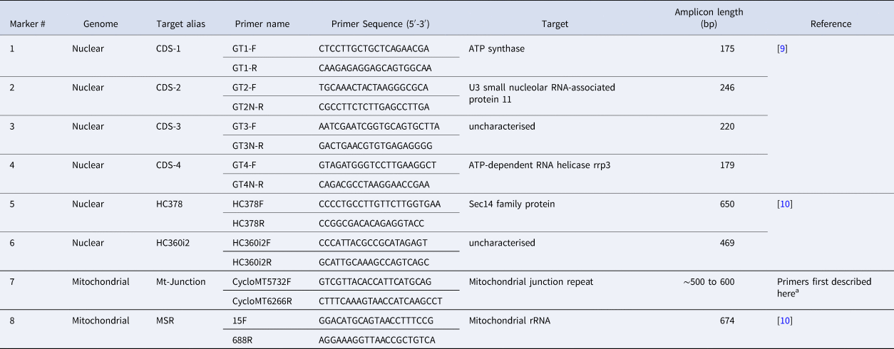
a These primers were modified from Nascimento et al. [Reference Nascimento11] to improve our amplification success rate, although the resulting amplicon still captures the same Mt Junction repeat described by Nascimento et al. [Reference Nascimento11].
Traceback and epidemiologic investigations
Specimens were assigned to epidemiologically-defined cyclosporiasis clusters and linked to suspected food vehicles where possible using previously described methods [Reference Nascimento3]. A cyclosporiasis cluster was defined as at least two cases of cyclosporiasis, with at least one with laboratory confirmation, epidemiologically linked to a common source or exposure.
FDA prioritised situations in which multiple, unrelated persons report exposures to the same point-of-service and a common food item, and conducted traceback investigations by reviewing records from case-patients, retailers, distributors and importers. If specific lot information was not available for the purchased product, timelines were constructed using the most likely timeframes capturing the transfer of product from one responsible party to another.
DNA extraction and PCR amplification
At the CDC and TX laboratories, 2 ml of stool was transferred to a plastic conical tube and washed with Phosphate Buffered Saline (PBS) at pH 7.4 (Gibco, Life Technologies) Waltham, Massachusetts, USA. DNA was extracted from ~0.5 ml aliquots of washed stool using the UNEX-based method [Reference Qvarnstrom12]. The DNA was eluted in 80 μl of elution buffer and stored at 4 °C. DNA extraction protocols employed at other participating laboratories differed subtly based on available resources and were controlled for using the proficiency specimens tested by each laboratory. PCR primers (Table 1) were synthesised at CDC and sent to the TX laboratory, while MN and NY used primers synthesised by LGC Biosearch Technologies (Petaluma, CA, USA) and Integrated DNA technologies (Coralville, Iowa, USA), respectively. Due to differences in the equipment available at each laboratory (i.e. thermocyclers, centrifuges, etc.), the optimised PCR protocols differed slightly between laboratories. The PCR protocols used at NY, MN and TX are described in detail in Supplementary File S1. The PCR protocol utilised at CDC to amplify CDC's eight genotyping markers is described in our previous work [Reference Nascimento3], using the primers provided in Table 1; the primer sequences for marker 7 were modified slightly here compared to our previous study [Reference Nascimento3]. At the CDC, NY and TX laboratories, sequencing was attempted on all PCR products, irrespective of whether an amplicon was visible following agarose gel electrophoresis. At the MN laboratory, PCR products for which multiple strong bands were visible following agarose gel electrophoresis were sequenced after excision of bands from gels. PCRs using water instead of DNA template were included with every PCR run as negative controls. Illumina sequencing was attempted at each marker for these negative samples. Methods, including the deep-amplicon sequencing methods used by each laboratory (CDC, TX, MN and NY) to generate the Illumina data, including the specific details on library preparation, are provided in Supplementary File S1.
Descriptions of modules 1 to 3
The descriptions provided in this manuscript give a general overview of the functions performed by each of the three modules comprising the genotyping workflow. These three modules each perform an essential task that ultimately facilitates the identification of infections caused by genetically related parasites (i.e. genetic clusters) for downstream epidemiologic follow-up:
Module 1: Assigns haplotypes to each specimen. This module will also detect and validate novel haplotypes that have not been encountered previously and will write them to a local database. Prior to 2019, 78 haplotypes had been identified across all CDCs genotyping markers [Reference Houghton9–Reference Nascimento11] (Supplementary File S1 – Appendix A). This includes the haplotypes defined at each sub-segment following the in-silico division of amplicons of markers 1–6, and marker 8 into segments of 100 base-pairs (or close to 100 base-pairs) so that each segment is treated as if it were a separate locus when haplotypes were defined. Splitting of full-length markers into smaller sub-segments was introduced to mitigate the impact of PCR-induced chimera formation on haplotype identification as we have discussed in detail elsewhere [Reference Barratt and Sapp13]. These 78 haplotypes were used as a reference database for priming Module 1: all haplotypes encountered in a specimen are compared to this reference database and if any of the haplotypes are novel, Module 1 expands the set of reference haplotypes to include this novel sequence by writing it to file.
Module 2: Examines the genotype information generated by Module 1 and assesses the relationship between each possible pair of specimens using this genotyping information. This second module is based on an updated version of the Barratt-Plucinski ensemble described in detail here: https://github.com/Joel-Barratt/Eukaryotyping [Reference Nascimento3, Reference Barratt10, Reference Barratt and Sapp13]. The Barratt-Plucinski ensemble comprises two machine learning algorithms that calculate a set of distances for each isolate pair. These distances are normalised as previously described [Reference Nascimento3] to generate an ensemble distance matrix that can be clustered for downstream analysis. Distances are computed by the ensemble based on the numbers of haplotypes shared between pairs of isolates, and all values computed fall between 0 and 1. The distances constitute a type of genetic distance where values close to (or equal to) 0 reflect high genetic similarity (i.e. many shared haplotypes) and a low chance that a pair is not of the same strain. A distance of 1 reflects low genetic similarity (i.e. few or no shared haplotypes) and a low chance that the pair of strains is genetically related. Detailed descriptions of these algorithms have been published elsewhere [Reference Nascimento3, Reference Barratt10, Reference Barratt and Sapp13].
Module 3: Predicts the most appropriate number of discrete genetic clusters in the population under analysis using a set of reference specimens of known genetic linkage. Essentially, this reference population is used to determine the ideal ‘within-cluster’ distance that would reflect a close genetic relationship. For this purpose, the present study used a set of specimens that were genotyped during the cyclosporiasis peak-period of 2018 and assigned to one of two major epidemiologic clusters; Vendor A (2018) and Vendor B (2018); 99 and 104 genotypes from each of these epidemiologic clusters respectively were re-analysed bioinformatically alongside specimens from 2019 (n = 875). These specimens represent ‘true positives’ given that they were genetically linked in agreement with their epidemiologic linkage, based on definitions described previously [Reference Nascimento3]. Briefly, identifying specimens that were both genetically linked and epi-linked (i.e. true positives) for this purpose involved clustering them as previously described [Reference Nascimento3]. The resultant dendrogram was then dissected at a level that maximised the assignment of specimens to the same genetic cluster as their epi-linked partners. Specimens epi-linked to the largest epidemiologic clusters from 2018 (i.e. Vendor A and Vendor B) that remained genetically linked following this empiric dendrogram dissection process were selected as ‘true positives’ to be included as the reference population for Module 3. Module 3 will output the number of defined clusters, as well as the cluster membership of each specimen in the analysis.
Performance assessment of the CDC genotyping system
We assessed performance by calculating a range of performance metrics including sensitivity, specificity, positive predictive value (PPV), NPV and accuracy as previously described [Reference Nascimento3], noting that sensitivity is the same as concordance as defined below:

where ClusterE is the number of specimens in an epidemiologic cluster, and ClusterG is the number of specimens in an analogous genetic cluster. For all calculations, epidemiologic clusters were empirically divided into two categories; category 1: epidemiologic clusters with six or more associated case-specimens genotyped, and category 2: epidemiologic clusters with less than six associated case-specimens genotyped. Only category 1 clusters were used to assess performance. The rationale for this is that epidemiologic clusters for which very few case-specimens were genotyped can greatly bias the performance metrics calculated if these are considered. For instance, an epidemiologic cluster with typing results for only two case-specimens that were each assigned to the same genetic cluster represents a 100% concordant result, despite that this cluster was represented by only two specimens. Similarly, an epidemiologic cluster for which only three case-specimens were typed and assigned to three different genetic clusters results in 0% concordance, negatively impacting how performance is perceived despite representing only three case-specimens. Epidemiologic clusters represented by a single genotyped case-specimen cannot be used to assess performance because a single specimen does not constitute a cluster.
The average was calculated across all epidemiologic clusters for each performance metric. Additionally, each metric was also weighted (Mweighted) by the ratio of the number of genotyped specimens in an epidemiologic cluster to the total number of genotyped specimens in category 1 (total = 365), using the following equation:
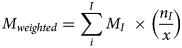
where I is the Ith epidemiologic cluster, MI is the percentage value obtained for the metric that is currently being weighted (i.e. sensitivity, specificity, PPV, NPV or accuracy) for the Ith epidemiologic cluster, nI is the number of specimens genotyped from the Ith epidemiologic cluster, and x is the number of specimens with epidemiologic links that were genotyped considering only epidemiologic clusters i to I.
As epidemiologic data were not available for all specimens genotyped, we assessed whether each genetic cluster was supported temporally by examining the illness onset dates of case-patients who provided a genotyped specimen. Using these illness onset dates, we generated separate epidemiologic curves for each genetic cluster to examine whether genetically-linked specimens also possess a temporal relationship.
We also assessed the discriminatory power of CDC's genotyping system using Simpson's index of diversity (D) as described elsewhere [Reference van Belkum14]. The value of D was determined by:

where N was considered the number of Cyclospora-containing faecal specimens genotyped (1078 specimens: 203 from 2018 and 875 from 2019), S was considered the number of distinct genetic types (clusters) identified (21 genetic clusters in this study – see results), and n j represents the number of Cyclospora-containing faecal specimens assigned to the jth genetic cluster. Values for n 1 to n 21 can be extracted from Supplementary File S2, Table C.
Data visualisation
The distance matrix generated using Module 2 was clustered by hierarchical agglomerative nesting (AGNES), in the R package ‘cluster’, version 2.0.6. AGNES was performed using Ward's method [Reference Strauss and von Maltitz15] with other parameters set to default. The resulting hierarchical tree was visualised using the R package ‘ggtree’. The un-clustered matrix was also visualised using MicrobeTrace (https://github.com/CDCgov/MicrobeTrace) [Reference Campbell16].
Human ethics
This activity was reviewed by CDC and was conducted consistent with applicable federal law and CDC policy.§ (Center for Global Health Human Research Protection Office determination number 2018-123).
Results
Specimens processed
By the end of 2019, participating state laboratories had sequenced 680 specimens submitted to their respective state health departments (NY; 381 specimens, TX; 267 specimens, MN; 32 specimens), and CDC had received 430 specimens from other US states. In total, 1110 faecal specimens were processed for genotyping in 2019, either at CDC or one of the three participating State laboratories. Our analysis confirmed that 875 of these specimens contained enough parasite material and/or yielded sequence data of sufficient quality for successful genotyping. By the end of 2019, 65 new haplotypes were detected in addition to the 78 known haplotypes. For specific details, please refer to Supplementary File S1, Appendices A and B. The ensemble distance matrix calculated by Module 2 is visualised in Figures 1 and 2. Module 3 predicted 21 genetic clusters.
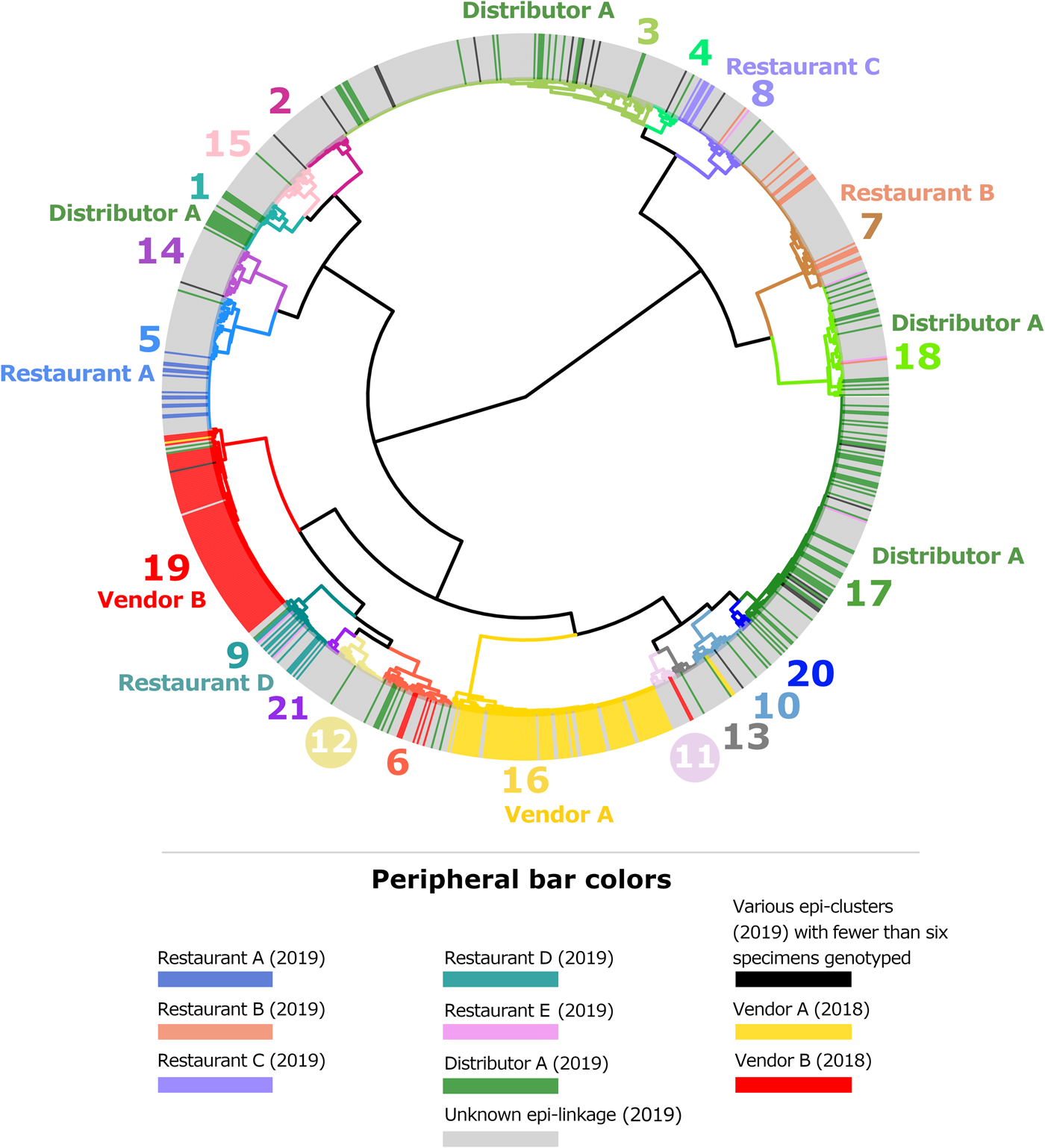
Fig. 1. Cluster dendrogram generated from the ensemble matrix of pairwise distances. An ensemble matrix calculated from 1078 C. cayetanensis genotypes (203 from 2018 and 875 from 2019) was clustered using Ward's method to generate the dendrogram shown. A cluster number of 21 was predicted by Module 3, and branches are numbered and colour-coded to reflect each respective cluster. Peripheral bar colours indicate specimens from case-patients epidemiologically linked to clusters of cyclosporiasis identified in the USA in 2018 or 2019, where at least six specimens were genotyped; colours of these bars reflect the specimen's epidemiologic linkages per the legend. Genetic clusters possessing a clear association with an epi-cluster have that epi-cluster's name labelled adjacent to the appropriate genetic cluster. The number of specimens assigned to each of the 21 genetic clusters is as follows: genetic cluster 1 (n = 30 specimens), cluster 2 (n = 26), cluster 3 (n = 175), cluster 4 (n = 15), cluster 5 (n = 72), cluster 6 (n = 40), cluster 7 (n = 80), cluster 8 (n = 42), cluster 9 (n = 32), cluster 10 (n = 31), cluster 11 (n = 13), cluster 12 (n = 28), cluster 13 (n = 13), cluster 14 (n = 28), cluster 15 (n = 27), cluster 16 (n = 112), cluster 17 (n = 134), cluster 18 (n = 61), cluster 19 (n = 104), cluster 20 (n = 7), cluster 21 (n = 8).
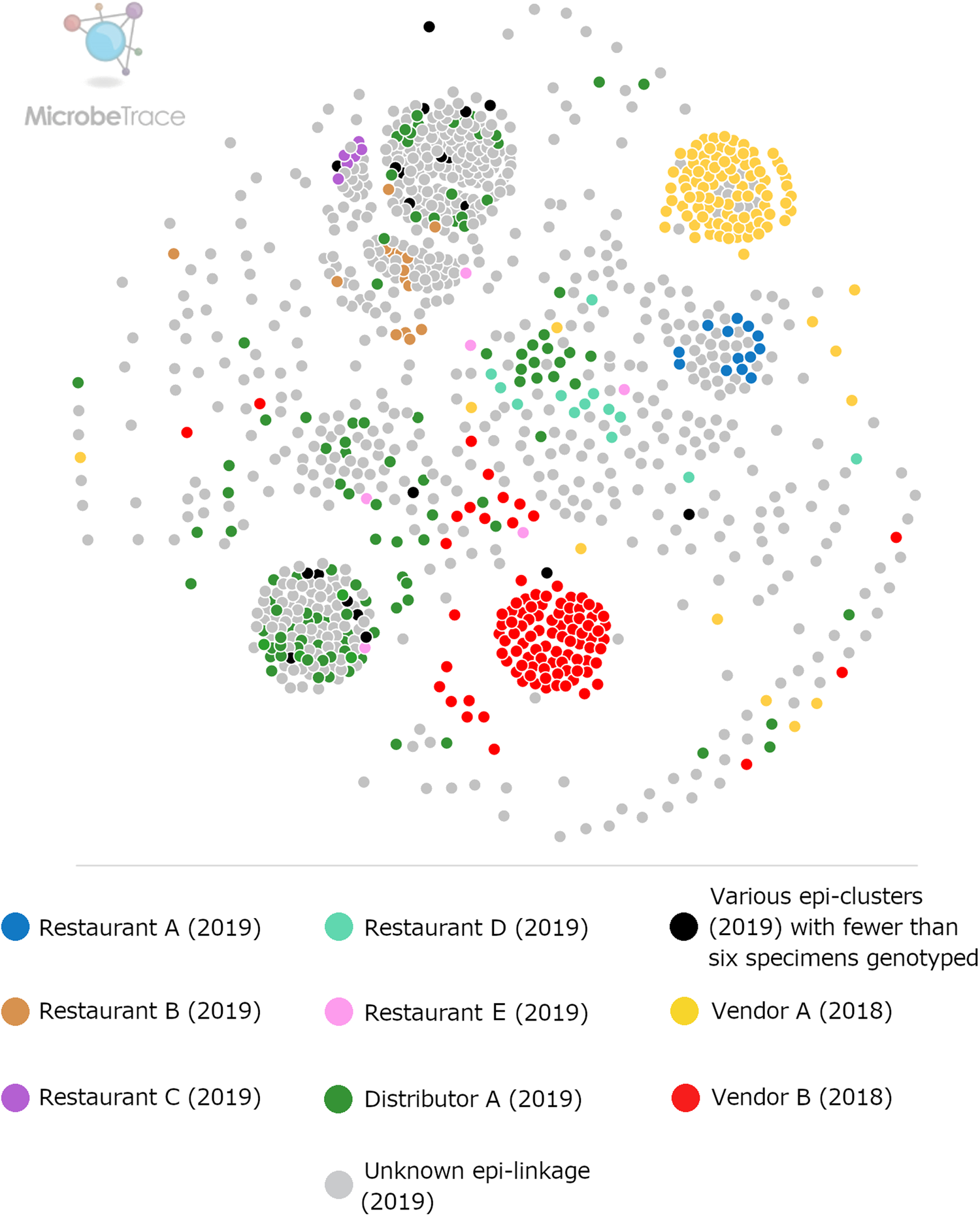
Fig. 2. Ensemble pairwise distance matrix visualised using MicrobeTrace. To generate this network the same ensemble matrix used to construct Figure 1 (Supplementary File S2, Table E) was filtered to a value of 0.11 using MicrobeTrace (https://github.com/CDCgov/MicrobeTrace/wiki). Nodes are colour-coded according to their epidemiologic linkage, using the same colours used to denote epidemiologically-defined clusters in Figure 1.
Defining epidemiologic clusters to assess genotyping performance
Based on epidemiologic investigations performed by state health departments in conjunction with FDA traceback efforts, 187 of the 875 genotyped specimens were linked to 14 epidemiologic clusters.
Six epidemiologic clusters fell into category 1 and were assigned the names ‘Distributor A’, ‘Restaurant A’, ‘Restaurant B’, ‘Restaurant C’, ‘Restaurant D’ and ‘Restaurant E’, noting that the large multistate outbreak associated with Distributor A involved infections linked to 23 restaurants and a single event where fresh basil was supplied by this distributor. Specimens linked to these six category 1 clusters comprised most specimens with epidemiologic links (167/187, 89%). Five of these clusters were used for the evaluation; Restaurant E was excluded from analysis because of a lack of concordance among the six specimens genotyped in the cluster – see Table 2 notes. Eight epidemiologically-defined category 2 clusters were excluded from downstream analysis and comprised only 20 case-specimens. For discussion of genotyping results obtained for these category 2 clusters, please refer to Supplementary File S1.
Table 2. Assessment of the ensemble performance against each epidemiologic cluster
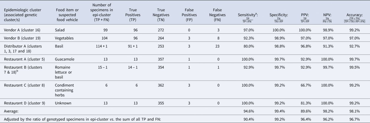
NPV, negative predictive value; PPV, positive predictive value.
Note: Despite being assigned to category 1, Restaurant E was not included in these calculations. Restaurant E is a chain specializing in fresh salads and the range of produce items consumed by some Restaurant E case-patients overlapped but varied, impeding the identification of a single food vehicle. Further, if a single food vehicle is not identified for a cluster, traceback is not conducted. Consequently, it is possible that some of these cases had different exposures at the same restaurant.
TP: Specimens linked to an epidemiologic cluster that were also assigned to the same genetic cluster.
TN: Using Vendor A as an example, this includes specimens linked to an outbreak other than Vendor A that were not assigned to genetic cluster 16.
FP: Using Vendor A as an example, this includes specimens linked to an outbreak other than Vendor A that were assigned to genetic cluster 16.
FN: Using Vendor A as an example, this includes specimens linked to the Vendor A outbreak that were not assigned to genetic cluster 16.
a Sensitivity values are identical to values of concordance based on the definition of concordance used in this study.
b 73% of case-patients associated with this epidemiologic cluster reported co romaine lettuce. Consumption of basil was reported by 25% of case-patients associated with this epidemiologic cluster. One of these specimens was assigned to genetic cluster 18 which was strongly linked to basil supplied by Distributor A. Consequently, we considered this single assignment to genetic cluster 18 to also be a concordant result. Therefore, we subtracted 1 case from the restaurant B cluster and added it to the Distributor A cluster as indicated in the table.
Figures 1 and 2 show the clustering of genotypes associated with the six category 1 epi-clusters from 2019 alongside the two reference clusters from 2018. Genotyped specimens associated with the category 2 epi-clusters (excluded from comparative analysis) are also shown (in black) in Figures 1 and 2. Many genotypes associated with various category 2 epi-clusters clustered genetically with certain category 1 epi-clusters – most of these category 2 specimens were assigned to genetic clusters 17 and 3 associated with basil linked to Distributor A (Fig. 1). Despite this, for these category 2 specimens, epidemiologic data did not support or failed to uncover a link to basil supplied by Distributor A.
Temporal relationships among genetically linked specimens
The epidemiologic curves for each genetic cluster supported temporal relationships for multiple genetic clusters (Fig. 3). However, genetic clusters 4, 13, 16, 19 and 21 had no clear peak illness onset date (i.e. no mode onset date). Genetic clusters 16 and 19 were predominantly linked to Vendor A (2018) and Vendor B (2018), respectively, and contained very few case-specimens from 2019 (Supplementary File S2, Table C). Similarly, genetic clusters 4, 13 and 21 contained 15 specimens or fewer, with only a subset of these specimens associated with a reported illness onset date (Supplementary File S1, Table D). Genetic clusters 2, 6 and 12 had a mode onset date, though the difference between the median and mode onset dates was one week or more for these clusters; 33, 10 and 7 days, respectively. For genetic clusters 1, 3, 5, 7, 8 to 11, 14, 15, 17, 18 and 20, the difference between the median and mode illness onset dates was less than one week, supporting a point-source exposure for the genetically linked cases within each of these genetic clusters (Fig. 3). Genetic cluster 20 contained only seven specimens, and only four had a reported illness onset date available. Clusters 1, 3, 5, 7, 8, 9, 17 and 18 possessed case-specimens with exposure data linking them to epidemiological clusters of cyclosporiasis (Figs 1 and 2).
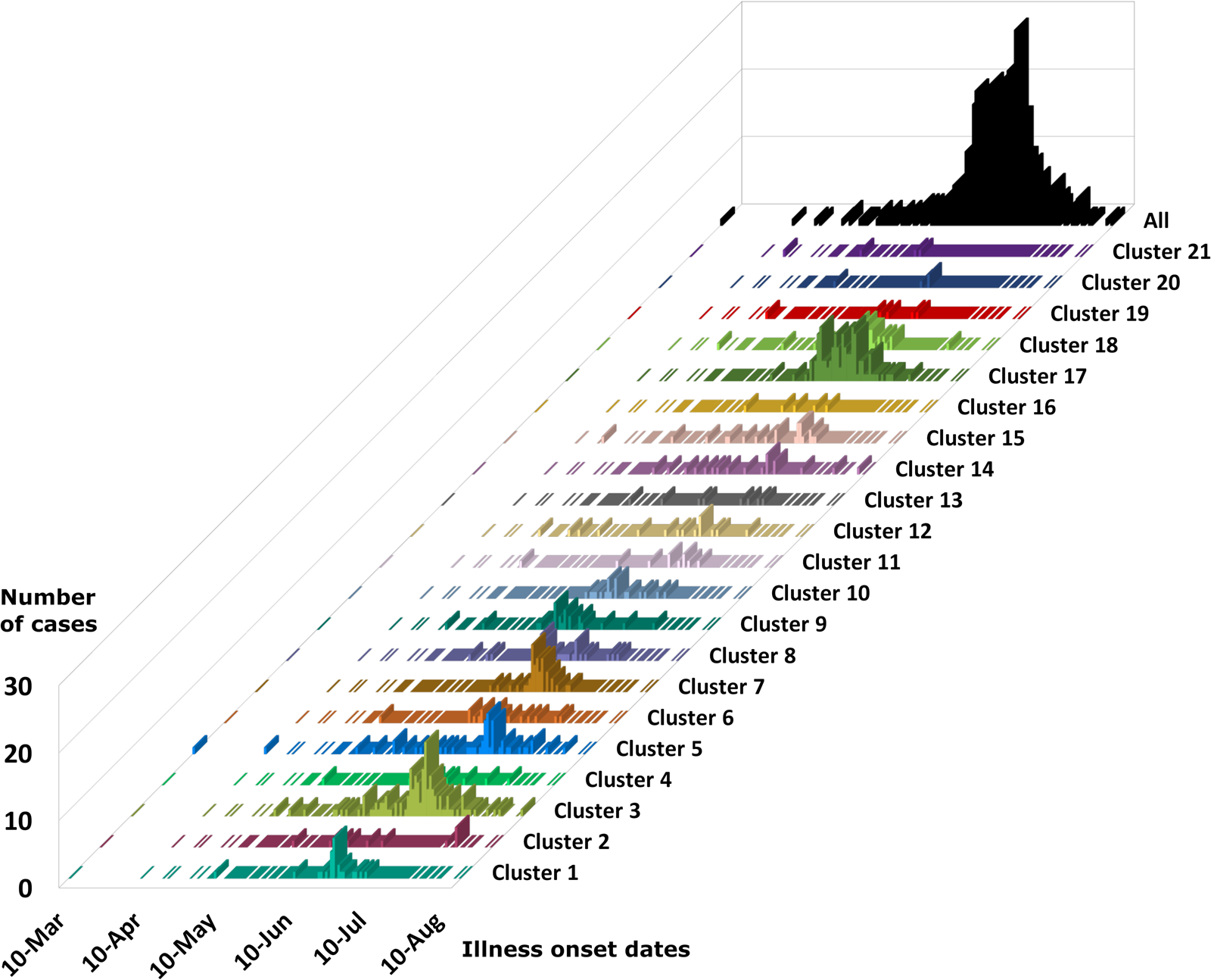
Fig. 3. Epidemiologic curves for cyclosporiasis cases plotted for each genetic cluster. Onset of illness dates for cases of cyclosporiasis is plotted as a separate histogram for each genetic cluster. Temporal clustering by genotype is supported, although there is substantial overlap in the temporal occurrence of several clusters. For the specific illness onset dates associated with each case-specimen refer to Supplementary File S2, Table C and Table D.
Cases associated with genetic clusters 1 and 18 peaked at a similar time, as did cases associated genetic clusters 3 and 17 (Fig. 4). These four genetic clusters were epidemiologically associated with basil supplied by Distributor A.
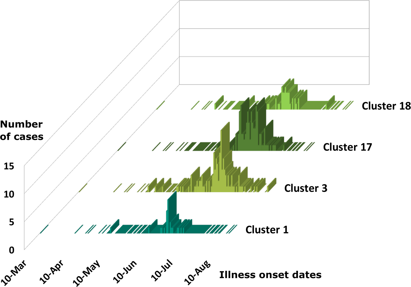
Fig. 4. Epidemiologic curves for cyclosporiasis cases for genetic clusters associated with Distributor A only. Illness onset dates for cases of cyclosporiasis are plotted as a separate histogram for each genetic cluster. This figure shows overlapping but distinct peak onset dates for each of these genetic clusters. The mode illness onset dates for genetic clusters 1 and 18 are similar; 25 June 2019, and 23 June 2019, respectively. The mode onset dates for genetic clusters 3 and 17 are also similar; 7 July 2019, and 4 July 2019, respectively.
Traceback
Thirteen epidemiologic clusters with an identified common source of basil were subject to full traceback. Distributor A was identified as supplying basil to 12 of the 13 restaurants or events associated with epidemiologic clusters. These include E1, R1, R5, R7, R9, R10, R12, R13, R14, R17, R19 and R21 – these 12 restaurants/events are referred to in Table 3 along with 12 others associated with Distributor A that were not subjected to full traceback (total = 24). Three discrete customers of Distributor A indirectly supplied these 12 epidemiologically-defined restaurant clusters through their respective distribution networks. The epidemiologic cluster that was not linked to basil from Distributor A did not have specimens included in the genotyping analysis and will not be discussed further. For six of the 12 epidemiologically-defined basil-associated clusters, additional suppliers could explain the basil available at the time of case exposure; however, when considering alternative suppliers to Distributor A as the source of illnesses, it should be noted that: (1) no single alternative supplier could explain more than two of these epidemiologic clusters; and (2) Distributor A is the sole likely supplier for six of these epidemiologic clusters.
Table 3. Breakdown of cases linked to Distributor A by restaurant/event and genetic cluster
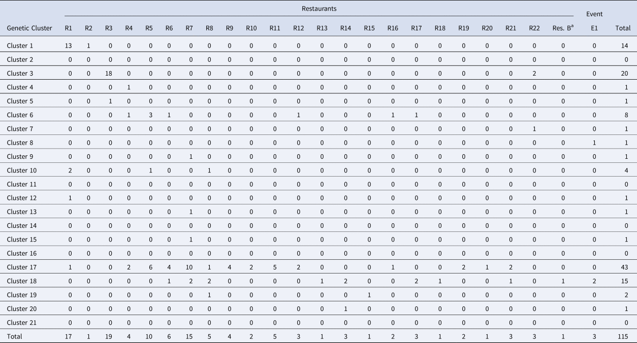
Note: Restaurant (R) or Event (E) where fresh basil was supplied by Distributor A based on traceback information. Most specimens associated with Distributor A were assigned to either of genetic clusters 1, 3, 17 and 18.
a Denotes Restaurant B. Most (73%) case-patients associated with Restaurant B consumed romaine lettuce, though 25% describe consuming basil. One genotyped specimen associated with Restaurant B was assigned to genetic cluster 18 which contains a large proportion of genotyped specimens associated with basil.
Additional epidemiologic clusters associated with basil were also investigated from a traceback perspective, but full documentation was not collected and analysed due to the product most likely being off the market through either previous product recalls or expiration of product. This is particularly relevant for epidemiologic clusters where the preliminary information suggested Distributor A may have been the supplier and actions to protect public health had already been taken regarding Distributor A's product at the time the information was received. Though less-thoroughly documented, R2, R3, R4, R6, R8, R11, R15, R16, R18, R20 and R22 were likely supplied with basil by Distributor A (Table 3). Five additional restaurants were identified as recipients of basil from Distributor A, and of these, one is included in the Category 2 clusters described above while the remaining four did not have any genotyping analysis performed on associated specimens. Two additional epidemiologic clusters where basil was identified as the common item were investigated, and a basil supplier other than Distributor A was identified; no genotyping analysis was conducted on these epidemiologic clusters.
In 2019, five epidemiologic clusters where cilantro was identified as a common source were investigated. No common source of cilantro was identified among all five epidemiologic clusters, but two restaurants, including Restaurant A and another epidemiologic cluster with no genetic analysis, received cilantro from a single source, while two others, including two clusters included in Category B below received cilantro from a common source that was different from the source for the first two. One epidemiologic cluster had no apparent traceback overlap with either common source with respect to cilantro supplied to the restaurant. No traceback information was collected for four category 2 clusters (Restaurants B, C, D and E).
Performance assessment
Performance analysis included 364 specimens with links to a total of seven epidemiologically-defined cyclosporiasis clusters (five category 1 epi-clusters from 2019 and two reference clusters from 2018). The epidemiologic cluster associated with Distributor A was associated with at least four genetic types of C. cayetanensis (Table 3). The other four category 1 epidemiologic clusters were each associated with a single genotype (Figs 1 and 2).
The concordance for these seven epi-clusters ranged between 80% and 100% (Table 2), noting that cases associated with Restaurant B were linked to one of two possible food vehicles; 73% of 44 case-patients linked to this cluster reported consuming Romaine lettuce, 25% reported basil, and 2% reported other food items. One specimen was assigned to genetic cluster 18 (associated with basil), while 13 specimens were assigned to genetic cluster 7. Despite the different genotypes detected for Restaurant B, this result was still considered concordant as the result supported the epidemiologic information (Table 3).
Performance metrics including sensitivity, specificity, PPV, NPV and accuracy for each epidemiologic cluster are shown in Table 2. Weighted values calculated for each metric were 90.4%, 99.2%, 96.4%, 96.2% and 96.6%, respectively. The discriminatory power (Simpson's index of diversity (D)) was 0.9173.
Discussion
We recently introduced several improvements to a C. cayetanensis genotyping system developed within the Parasitic Diseases Branch at CDC [Reference Nascimento3, Reference Barratt10]. These improvements include the addition of a workflow that discovers novel haplotypes (Module 1); the inability to identify novel haplotypes was a major limitation of the original workflow [Reference Nascimento3]. Each of Modules 1 through 3 allows users to supply a range of arguments that can be customised if needed (Supplementary File S3). The increased automation of this workflow supports the system's national deployment potential across multiple US public health laboratories. While Modules 1 through 3 will require adjustment as the field of computational biology evolves, this work represents an important step towards a national C. cayetanensis genotyping system. However, due to these modifications, a re-evaluation of the system was warranted to exclude the possibility that these changes negatively impacted its performance relative to our earlier evaluation [Reference Nascimento3]; this was the main impetus for the present study.
Taking advantage of the large C. cayetanensis MLST dataset generated in 2019, in conjunction with data generated in 2018, the performance of this updated system was assessed. Here, Module 3 predicted a population structure comprising 21 genetic clusters and using these genetic clusters, values for sensitivity, specificity, PPV, NPV and accuracy were calculated; these values were high, and were similar to those of the prior evaluation of an earlier version of this system [Reference Nascimento3].
The inclusion of data from 2018 in this analysis served two purposes. First, data from a reference population of known genetic and epidemiologic linkage were required for Module 3 to predict an appropriate number of genetic clusters. Second, the inclusion of 2018 data increased the size and complexity of the dataset while providing a set of specimens that clustered correctly in a previous evaluation [Reference Nascimento3]. These specimens served as a control population allowing us to assess whether these same specimens clustered together correctly in the context of a different dataset and a modified workflow. Given the strong performance of the updated system and the appropriate clustering of the 2018 reference genotypes, no discernable negative impacts on performance were observed since our original evaluation [Reference Nascimento3]. Furthermore, the excellent performance characteristics reported here likely represent a lower-boundary estimate of the system's true performance as all metrics were calculated assuming the epidemiologic data to be error-free.
Our previous study proposed a 10-genetic cluster population structure as determined using the epidemiologic and genotyping data available at the time [Reference Nascimento3]. The 21-cluster model supported here reflects a higher level of discriminatory power than the earlier 10-cluster population structure [Reference Nascimento3] and supports the ability of this method to detect a wide range of genetic variants that can be clustered into distinct populations. To quantify the discriminatory power of our system in this study, we calculated Simpson's index of diversity (D) and obtained a value of 0.9173. An ideal genotyping procedure would possess a Simpson's index of between 0.95 and 1.00 [Reference van Belkum14], so a value of D = 0.9173 reflects good discriminatory power, with potential for improvement. However, given that the present dataset describes only the second year of wide-scale C. cayetanensis genotyping in the USA, we assume that our 21-cluster population structure likely represents an under-estimation of the diversity of C. cayetanensis genotypes; our datasets are heavily biased towards C. cayetanensis types detected during the cyclosporiasis peak-periods of 2018 and 2019. Therefore, the number of genetic clusters, and the value of D, will likely increase as more samples are analysed over time.
Comparison of numerous epidemiologically-defined clusters to their analogous genetic clusters has confirmed that what constitutes a closely related C. cayetanensis ‘type’ is pliable, and that isolates assigned to the same ‘genetic cluster’ do not necessarily possess precisely the same genotype [Reference Nascimento3,Reference Barratt10]. We previously proposed that this was due to the sexual reproductive cycle of C. cayetanensis [Reference Barratt10], which was the impetus for the development of our ensemble-based distance statistic (now included as part of Module 2), that facilitates the analysis of complex, highly heterozygous, genotyping data (discussed elsewhere: [Reference Nascimento3,Reference Barratt10,Reference Barratt and Sapp13]). Regardless, assignment of two genotyped specimens to the same genetic cluster using CDC's system does not necessarily mean that their genotypes are identical. This is an important consideration when discussing infections caused by genetically-similar parasites.
This study highlights a novel phenomenon regarding the logistics of C. cayetanensis dispersion throughout fresh produce supply chains in the USA. In 2018, two major outbreaks were traced back to separate vendors of produce (Vendor A and Vendor B), caused by two separate genetic types of C. cayetanensis – one type was implicated in each outbreak and genotypes identified associated with these outbreaks were included here as part of our reference population. The same dynamic was observed for other cyclosporiasis clusters observed in 2018: Restaurants A (2018) and B (2018) shared their supplier of herb 1, a supplier associated with a single C. cayetanensis type [Reference Nascimento3]. Two cases linked to the Restaurant C (2018) cyclosporiasis cluster were attributed to the same type, as were eight of 10 cases linked to Temporospatial cluster A (2018) [Reference Nascimento3]. Among the five main epi-clusters from 2019, three were attributed to a single type. Three types were implicated in the Restaurant B (2019) cluster – one specimen was assigned to genetic cluster 8, another to genetic cluster 18, while the remaining 13 specimens were assigned to genetic cluster 7. The epidemiologic data supported that Restaurant B (2019) cases may have been associated with two food vehicles of cyclosporiasis: romaine lettuce and basil, and genetic cluster 18 (where one Restaurant B case-specimen was assigned) was strongly associated with a basil exposure (Table 2). The single specimen assigned to genetic cluster 8 was considered a false-negative for the Restaurant B (2019) cluster. Thus, we typically observe that cyclosporiasis outbreaks associated with a specific restaurant or event are associated with a single genetic type of C. cayetanensis.
By contrast, while Restaurant E fell into category 1, it was excluded from downstream performance evaluations due to the lack of concordance among the six case-specimens genotyped for this cluster along with the absence of an identified food vehicle. As a result, these data were not included in the performance evaluations. Restaurant E is a chain specializing in fresh salads and the range of produce items consumed by some Restaurant E case-patients overlapped but varied, impeding the identification of a single food vehicle. Further, if a single food vehicle is not identified for a cluster, traceback is not conducted. Consequently, it is possible that some of these cases had different exposures at the same restaurant. One of six Restaurant E case-specimens was assigned to genetic cluster 8, two were assigned to genetic cluster 9, another was assigned to genetic cluster 17, and two were assigned to genetic cluster 18. Genetic cluster 9 contained all case-specimens linked to Restaurant D (Supplementary File S2, Table C), and onset dates and location (state) for these Restaurant D cases were consistent with the two cases from Restaurant E also assigned to cluster 9. This could imply a shared vehicle despite exposure at different restaurants; a vehicle also was not identified for Restaurant D and traceback was limited due to the lack of a single identified vehicle. The Restaurant E specimens assigned to genetic clusters 17 and 18 were associated with basil supplied by Distributor A. Distributor A also supplied fresh herbs to the U.S. beyond basil. Given this, it's also possible that Restaurants D and E shared a common non-basil ingredient supplied by Distributor A or another supplier.
Cases linked to basil supplied by Distributor A (2019) were attributed to at least four main C. cayetanensis types (Table 3), and we can probably attribute this to the scale of operations performed by Distributor A. Given that Distributor A is an international distributor of fresh herbs, this may not be unreasonable, and similar scenarios with multi-serotype foodborne outbreaks caused by bacterial pathogens have been documented previously [Reference Hassan17, Reference Crowe18]. It seems possible that multiple C. cayetanensis types would contaminate a sufficiently large volume of basil during a single contamination event, or that multiple, smaller, contamination events with different types may have occurred. Contamination events may occur at the farm or ranch where the produce is grown via contamination of soil or irrigation water with faeces from multiple individuals (i.e. persons infected with different Cyclospora types). As basil is generally distributed via air transport due to its perishability, it is not surprising to see such wide geographic dispersion through the eastern US. When several small epi-clusters first emerged in 2019 in association with various restaurants, the Cyclospora types identified in case-specimens linked to these restaurants were sometimes (uncharacteristically) conflicting; a single restaurant-cluster was sometimes associated with multiple Cyclospora types. It was not until traceback data became available that patterns began to emerge. Many of these restaurants were supplied with basil by Distributor A which was associated with four Cyclospora types (Table 3); some case-patients whose illnesses were linked to a particular restaurant exposure were infected with one of the four types, though not necessarily with the same type as other case-patients who become infected after eating at the same restaurant. Key examples of this phenomenon include cases linked to Restaurants R6, R7, and R8 (Table 3), where case-specimens were assigned to either of genetic clusters 17 or 18; these examples suggest that a single contamination event with multiple types occurred. Conversely, traceback demonstrates that a single lot of product cannot explain all illnesses associated with basil from Distributor A, suggesting multiple contamination events occurred. Consequently, the outbreak associated with Distributor A highlights the importance of integrating traceback information with genotyping and epidemiologic data when investigating outbreaks of cyclosporiasis.
Basil is an extremely common herb, widely consumed in the USA. The widespread use of basil (and other herbs) presents challenges for epidemiologic investigations when these herbs are implicated as outbreak vehicles. Cyclosporiasis case-patients may not specifically report consuming basil when used as a side garnish or as a component of a salad, or may have become infected via consumption of a different component of the same meal. Response bias is another challenge, where case-patients are aware via the mass media or other sources, that a large multi-state cyclosporiasis outbreak is occurring because of a specific food vehicle. Another problem is the possibility for cross-contamination at the point of service: the preparation of fresh vegetables, leafy greens and herbs on the same surface using the same utensils without cleaning in between may lead to contamination of other vehicles, introducing additional noise to the epidemiologic data. Finally, the impact of these epidemiologic noise sources (for widely consumed produce items in particular) is compounded by recall bias. It can be difficult for patients to recall specific meal components consumed several weeks ago.
In 2019, despite these challenges, a clear signal was observed highlighting an association between numerous cyclosporiasis cases and basil provided by Distributor A. The present study was retrospective in nature: faecal specimens from 2019 were genotyped, genetic clusters were identified, and these genetic clusters were compared to analogous epidemiologic clusters to assess the performance of CDC's updated/modified genotyping system. However, if genotyping had been performed before epidemiologic data were available (i.e. in a blinded manner) and the genetic clusters identified were used to guide downstream epidemiologic investigations, a signal would have been detected for a common source, ultimately identified as Distributor A, using genotyping. Cyclosporiasis cases epidemiologically linked to Distributor A were scattered among genetic clusters 4 to 10, 12, 13, 15, 19 and 20, though at a low frequency compared to the four major types associated with Distributor A – the types represented by genetic clusters 1, 3, 17 and 18. It is possible that some case-specimens scattered among the seemingly unrelated clusters may have been linked to this outbreak due to one or more sources of epidemiologic error discussed previously. Regardless, despite this low-frequency scattering among many genetic clusters, dissecting the epidemiologic data by examining food histories among case-patients whose specimens were assigned to the same genetic cluster would have reduced the number of falsely linked cases (i.e. case-specimens from unrelated types with a low likelihood of sharing the same food vehicle). This would have also increased the signal for basil supplied by Distributor A when the food histories among case-specimens assigned to any of genetic clusters 1, 3, 17 and 18 were examined – the same phenomenon would have been observed for the four other major epidemiologic clusters from 2019 discussed here.
Similarly, better epidemiologic data equates to better traceback investigations with less uncertainty. Current traceback approaches to most enteric pathogen outbreak investigations rely on an underlying understanding that among cases who share a genetically similarly pathogen, there exists a common thread connecting these cases, such as a food, water source or animal exposure. If these genetic similarities are defined in real-time, investigators can focus resources on groups of illnesses that share genetic similarity and thus more easily identify a common source of C. cayetanensis. In the 2019 investigation associated with basil, most, but not all, of the restaurants or events could be explained by a single supplier, Distributor A. Ideally, those not associated with Distributor A could have been identified at the outset of the investigation as not likely to be related. Applying genetic sub-typing may also assist in identifying additional common sources attributed to smaller numbers of illnesses with different types (i.e. separate outbreaks) that would otherwise go without a traceback investigation.
Despite the promising results presented here, reliance on this method alone to guide epidemiology and traceback investigations must be approached with caution. Genetic cluster 3 is an example of where the results may raise more questions than answers. This genetic cluster contained specimens from R3 and R22, as well as five category 2 epidemiologic clusters where fewer than six specimens were genotyped. While R3 and R22 could have received basil from Distributor A, thorough documentation was not collected and the epidemiologic data linking R3 and R22 to basil supplied by Distributor A was less strong than for some other clusters. For two of the epidemiologic clusters from category 2, cilantro was the focus of traceback with a single supplier noted, while for a third category 2 cluster, a non-herb vehicle was considered. It is possible that a single farm source could account for this observation of multiple vehicles; however, it is also possible that if the genetic analysis was known at the outset of the outbreak investigation, a single vehicle source would have been sought, perhaps unsuccessfully so. Continued integration of genetic typing with epidemiologic and traceback data will allow investigators to better understand possible limitations in the method.
Despite these considerations, genotyping usually confirmed a genetic link among epidemiologically-linked case specimens. However, many case-specimens were not linked to a specific epidemiological cluster due to the absence of epidemiological data. For case-specimens with unknown epidemiological linkage, it is difficult to assess whether their assignment to a particular genetic cluster constitutes a correct assignment. While epidemiologic data were sometimes lacking, illness onset dates for case-patients were often available. These dates enabled an assessment of whether genetically linked case-specimens produced a typical epidemiologic curve when plotted against these onset dates; one would expect a unimodal curve with similar median and mode illness onset dates in the case of a single cyclosporiasis outbreak. In line with this rationale, epidemiologic curves plotted individually for each genetic cluster supported the genetic relationships observed, adding additional credence to this genotyping procedure.
This study highlights the epidemiologic utility of CDC's C. cayetanensis genotyping system. Several bioinformatic improvements to our previously described workflow were introduced recently, including de novo detection of novel haplotypes and the ability of users to supply several custom arguments. Module 3 automatically predicts the cluster membership of specimens being analysed, which reduces the impact of human bias when assigning genetic links among case-specimens. Given these modifications, the present study assessed the performance of this modified genotyping system to ensure that no observable negative impacts on performance were introduced. We demonstrated that no negative impacts on performance were observed relative to an earlier iteration of our genotyping system which has now performed robustly for two consecutive years, and possesses good discriminatory power. Overall, this work represents a significant step towards a functional US-wide Cyclospora genotyping system that will facilitate detection of cyclosporiasis outbreaks in the future and enhance our understanding of the dynamics of C. cayetanensis dispersion throughout US fresh produce supply chains.
Supplementary material
The supplementary material for this article can be found at https://doi.org/10.1017/S0950268821002090.
Acknowledgements
The authors would like to acknowledge the assistance of the following people for their contribution to this study, either by providing post-diagnostic faecal specimens and/or providing additional epidemiologic meta-data that assisted in the generation of this manuscript: Jisun Haan. We also acknowledge the Wadsworth Center Advanced Genomic Technologies Cluster for library preparation and next generation sequencing, and the Texas Health Molecular diagnostic laboratory for their participation in this work.
Author contributions
JB wrote original drafts, designed and wrote bioinformatic workflows (custom code), designed data analysis procedures, designed figures, designed bioinformatic experiments, performed data analysis, and data interpretation. KH and TR performed laboratory work, including specimen organisation, DNA extraction, PCR, library preparation and assay optimisation. EC performed laboratory work including DNA extraction and PCR. BB, JK and CM performed laboratory work, including specimen organisation, DNA extraction, PCR at the NY Wadsworth State Health Department laboratory. SMA led the NY arm of the project. AS performed epidemiologic investigations, proofread early drafts and approved final drafts. RT compiled epidemiologic data, proofread early drafts and approved final drafts. VC co-led the project, participated in data interpretation and manuscript preparation, and approved the final draft. MJA and YQ approved the grant and led the project. BMW performed the traceback analysis and compiled the traceback information. KRK was the lead outbreak coordinator for FDA. All authors edited and approved the final manuscript draft.
Financial support
This research was supported by a grant from the Centers for Disease Control and Prevention Office of Advanced Molecular Detection.
Conflict of interest
None.
Disclaimer
The findings and conclusions in this report are those of the authors and do not necessarily represent the official position of the Centers for Disease Control and Prevention/the Agency for Toxic Substances and Disease Registry. The use of trade names is for identification only and does not imply endorsement by the Department of Health and Human Services or the Centers for Disease Control and Prevention.
Data
Raw reads generated for each specimen have been made publicly available by submission to NCBI under BioProject accession number PRJNA578931. All scripts required to run this workflow can be accessed at the following GitHub repository: https://github.com/Joel-Barratt/CDC-Complete-Cyclospora-typing-workflow-ALPHA-TEST. Detailed installation and usage instructions for this workflow are also provided in Supplementary File S3.


 Open access