


1 Introduction
A fundamental problem in fluid dynamics is the long-time resolution of a large localised disturbance. In inviscid fluids, a prominent feature of this resolution is the emergence of a solitary wavetrain. This process is generally referred to as soliton fission and has been observed in a variety of fluid contexts. For example, while intense earthquakes can lead to the vertical displacement of the ocean surface by several metres, its horizontal extent can reach 10–100 km (Geist et al. Reference Geist, Titov, Arcas, Pollitz and Bilek2007), which, under appropriate shallowness conditions, can evolve into a large number of surface solitary waves (Matsuyama et al. Reference Matsuyama, Ikeno, Sakakiyama and Takeda2007; Arcas & Segur Reference Arcas and Segur2012). Another important example is the generation of large-amplitude internal ocean solitary waves with two identified soliton fission mechanisms: (1) an initial broad displacement of internal temperature and salinity (Osborne & Burch Reference Osborne and Burch1980), and (2) the propagation of a large internal solitary wave onto a shelf (Farmer & Armi Reference Farmer and Armi1999; Vlasenko et al. Reference Vlasenko, Stashchuk, Inall and Hopkins2014). In both scenarios, the result is the same – the generation of a large number of rank-ordered solitary waves. In fact, the well-known soliton fission law by Djordjevic & Redekopp (Reference Djordjevic and Redekopp1978) for scenario 2 was obtained by modelling it with an initial broad disturbance to the constant-coefficient Korteweg–de Vries (KdV) equation, a weakly nonlinear long-wave model. More generally, the disintegration of a broad disturbance into solitary waves is the inevitable result of boundary or topography interaction with an undular bore or dispersive shock wave (DSW) that results from a sharp gradient due to a variety of reasons (El & Hoefer Reference El and Hoefer2016).
Despite the prevalence of soliton fission in fluid dynamics, its theoretical description has primarily been limited to completely integrable partial differential equations (PDEs) such as the KdV equation. First attempts to understand this problem began with the celebrated Zabusky–Kruskal numerical experiment of an initial cosine profile for KdV (Zabusky & Kruskal Reference Zabusky and Kruskal1965). Asymptotics of KdV conservation laws (Karpman Reference Karpman1967; Johnson Reference Johnson1973) and the inverse scattering transform (Segur Reference Segur1973; Deng, Biondini & Trillo Reference Deng, Biondini and Trillo2016) yield a prediction for the number of solitons based on eigenvalue counting and an estimate for the amplitudes of fissioned solitons from an initial profile.
Because of its ubiquity, we seek a deeper understanding of soliton fission that results from a broad initial condition, hereafter referred to as the box problem due to the initial profile’s wide shape. A new method based on Whitham averaging theory (Whitham Reference Whitham1974) that does not require integrability was first proposed and applied to the Serre/Su–Gardner/Green–Naghdi equations for fully nonlinear shallow-water waves in El, Grimshaw & Smyth (Reference El, Grimshaw and Smyth2008) and, partially, to the defocusing nonlinear Schrödinger equation with saturable nonlinearity in El et al. (Reference El, Gammal, Khamis, Kraenkel and Kamchatnov2007). The method draws upon principles first developed to describe DSWs that result from step initial data (El Reference El2005). The long-time evolution into a solitary wavetrain is one component of the soliton resolution conjecture, which proposes that localised initial conditions to nonlinear dispersive wave equations generically evolve into a soliton wavetrain and small-amplitude dispersive radiation, originally formulated within the context of integrable PDEs such as the KdV equation (Segur Reference Segur1973; Schuur Reference Schuur1986; Deift, Venakides & Zhou Reference Deift, Venakides and Zhou1994). Because the method presented here is not reliant on integrability of the underlying PDE and yields concrete predictions for the number of solitary waves and their amplitude distribution that result from broad initial disturbances, we refer to this approach as the solitary wave resolution method. An important feature of the solitary wave resolution method is that it bypasses an analysis of the full Whitham modulation equations – which are generally difficult to analyse – in favour of the exact zero-amplitude and zero-wavenumber reductions of the full Whitham equations that admit a general structure and form that is amenable to further analysis.
We note that the solitary wave resolution method does not resolve the second component of the soliton resolution conjecture – the small-amplitude dispersive radiation. For sufficiently broad boxes, this component of the conjecture is negligible, as is well known for the KdV equation (see e.g. Karpman Reference Karpman1974; Whitham Reference Whitham1974). We quantify the contributions of the radiation and solitary wave components numerically for a specific initial disturbance in the conduit equation.
Our basic hypothesis in this work is that a large initial disturbance in certain non-integrable equations (e.g. the conduit equation described below) results most prominently in the fission of solitary waves, which enables us to apply Whitham averaging theory (Whitham Reference Whitham1974). This hypothesis is motivated by rigorous semiclassical analysis of the KdV equation (Lax & Levermore Reference Lax and Levermore1979) and is confirmed by numerical simulations for the conduit equation. Moreover, this hypothesis has been successfully applied to the non-integrable Serre equations (El et al. Reference El, Grimshaw and Smyth2008).
The solitary wave fission problem has been studied experimentally, primarily in water wave tanks modelled by the KdV equation (Hammack & Segur Reference Hammack and Segur1974, Reference Hammack and Segur1978). More recent water wave experiments physically recreated the Zabusky–Kruskal numerical experiment, observing recurrence as well as soliton fission (Trillo et al. Reference Trillo, Deng, Biondini, Klein, Clauss, Chabchoub and Onorato2016). These experiments exhibit excellent agreement with Wentzel–Kramers–Brillouin (WKB) theory applied to the inverse scattering transform (Deng et al. Reference Deng, Biondini and Trillo2016). The WKB approach has also been applied to the defocusing nonlinear Schrödinger equation, yielding the number and amplitudes of emergent solitons (Deng et al. Reference Deng, Li, Biondini and Trillo2017). However, none of these quantitative methods are applicable to non-integrable equations.
This paper presents solitary wave fission experiments and modulation theory for the interfacial dynamics between two high-viscosity miscible fluids, one rising buoyantly within another. Original experiments demonstrated that solitary waves preserve their shape and form despite long-distance propagation and interaction with other solitary waves (Olson & Christensen Reference Olson and Christensen1986; Scott, Stevenson & Whitehead Reference Scott, Stevenson and Whitehead1986). In fact, in both of these experimental papers, solitary waves were generated by the fission of a large initial disturbance. We apply modulation theory for solitary wave fission introduced in El et al. (Reference El, Grimshaw and Smyth2008) to the box problem for a PDE model of this fluid context known as the conduit equation (Lowman & Hoefer Reference Lowman and Hoefer2013a)
 $$\begin{eqnarray}a_{t}+(a^{2})_{z}-(a^{2}(a^{-1}a_{t})_{z})_{z}=0.\end{eqnarray}$$
 In the derivation of the conduit equation, no restriction is placed on the magnitude of the non-dimensional circular cross-sectional area  $a(z,t)$, where $z$ and $t$ are the scaled height and time, respectively, assumed to be much larger than the conduit diameter and a characteristic advective time scale. This equation is also applicable to an asymptotic long-wave model of magma flows rising through the Earth’s mantle (Barcilon & Richter Reference Barcilon and Richter1986; Whitehead & Helfrich Reference Whitehead and Helfrich1988; Helfrich & Whitehead Reference Helfrich and Whitehead1990) and to a comparatively simple laboratory experiment (Olson & Christensen Reference Olson and Christensen1986; Scott et al. Reference Scott, Stevenson and Whitehead1986; Whitehead & Helfrich Reference Whitehead and Helfrich1988; Helfrich & Whitehead Reference Helfrich and Whitehead1990; Lowman & Hoefer Reference Lowman and Hoefer2013a; Maiden et al. Reference Maiden, Lowman, Anderson, Schubert and Hoefer2016, Reference Maiden, Anderson, Franco, El and Hoefer2018; Anderson, Maiden & Hoefer Reference Anderson, Maiden and Hoefer2019). Equation (1.1) fails the so-called Painlevé test for integrability (Harris & Clarkson Reference Harris and Clarkson2006) and has at least two conservation laws (Harris Reference Harris1996), and therefore is an excellent candidate to test the more broadly applicable solitary wave resolution method for the initial value problem consisting of (1.1) and
 $$\begin{eqnarray}a(z,0)=1+a_{0}(z),\quad \lim _{\left|z\right|\rightarrow \infty }a_{0}(z)=0,\end{eqnarray}$$
 where  $a_{0}(z)$ is a broad localised disturbance with exactly one critical point at the maximum
 $$\begin{eqnarray}a_{m}=\max _{z\in \mathbb{R}}a_{0}(z).\end{eqnarray}$$
 Note that  $a=a_{m}+1$ at the maximum, i.e. $a_{m}$ measures the amplitude of the disturbance exceeding the unit background area ratio $a=1$. We will quantify the profile’s broadness more precisely later on, but for $a_{0}(z)$ in the shape of a box, then a sufficiently wide box will do. Formally, $a_{0}\in {\mathcal{C}}^{\infty }(\mathbb{R})$ as well, but the relaxation of this assumption still aligns with the theoretical results. We shall assume that the support of $a_{0}(z)$ is $[-w,0]$, where $w>0$ is the box width. The solitary wave resolution method utilises the characteristics of the Whitham modulation equations to estimate the number of solitary waves and the solitary wave amplitude distribution resulting from a large-scale initial condition. An example initial condition and its numerically evolved state according to the conduit equation (1.1) are shown in figure 1. The theoretically predicted solitary wave number (12, derived in § 4) is correct and the predicted amplitudes fall well within the ranges determined from the quantisation of the continuous amplitude distribution (derived in § 5).

Figure 1. An example box initial condition (inset) and its long-time numerical evolution according to the conduit equation (1.1). The number in the inset denotes the predicted number of solitary waves from that initial condition based on the solitary wave resolution method, and the black circles with vertical bars denote the ranges from a quantiled distribution of the predicted solitary wave amplitudes, both derived later in this paper.
The conduit equation (1.1) can be approximated by the KdV equation
 $$\begin{eqnarray}u_{\unicode[STIX]{x1D70F}}+uu_{x}+u_{xxx}=0\end{eqnarray}$$
in the small-amplitude, long-wavelength regime with the scaling (Whitehead & Helfrich Reference Whitehead and Helfrich1986)
 $$\begin{eqnarray}\unicode[STIX]{x1D70F}=\unicode[STIX]{x1D6FF}^{3/2}t,\quad x=\unicode[STIX]{x1D6FF}^{1/2}2^{-1/3}(z-2t),\quad u=2^{2/3}\unicode[STIX]{x1D6FF}(a-1),\quad 0<\unicode[STIX]{x1D6FF}\ll 1,\end{eqnarray}$$
 where  $\unicode[STIX]{x1D6FF}$ is a characteristic disturbance amplitude deviation from unit background. The formulae for the expected number of solitons ${\mathcal{N}}$ and the amplitude ( ${\mathcal{A}}$) density function $f({\mathcal{A}})$ for the initial profile $u(x,0)=u_{0}(x)$ to the KdV equation (1.4) are (El et al. Reference El, Grimshaw and Smyth2008)
 $$\begin{eqnarray}\left.\begin{array}{@{}c@{}}\displaystyle {\mathcal{N}}=\frac{1}{\unicode[STIX]{x03C0}\sqrt{6}}\int _{-\infty }^{\infty }\sqrt{u_{0}(x)}\,\text{d}x,\\ \displaystyle f({\mathcal{A}})=\frac{1}{4\unicode[STIX]{x03C0}\sqrt{6}}\int _{x_{1}}^{x_{2}}\frac{\text{d}x}{\sqrt{u_{0}(x)-{\mathcal{A}}/2}},\quad 0\leqslant {\mathcal{A}}\leqslant 2u_{m}.\end{array}\right\}\end{eqnarray}$$
 Here,  $x_{1}$ and $x_{2}$ are the intersections of the initial condition $u_{0}$ with the value ${\mathcal{A}}/2$. The initial data are assumed to be on a zero background with maximum $u_{m}=\max u_{0}(x)$. For initial data consisting of a box of width $w$ and height $u_{m}$, equation (1.6) becomes
 $$\begin{eqnarray}\left.\begin{array}{@{}c@{}}\displaystyle \text{for}~u_{0}(x)=\left\{\begin{array}{@{}ll@{}}u_{m}\quad & -w<x<0,\\ 0\quad & \text{else},\end{array}\right.\quad {\mathcal{N}}=\frac{w\sqrt{u_{m}}}{\unicode[STIX]{x03C0}\sqrt{6}},\\ \displaystyle {\mathcal{F}}({\mathcal{A}})=\frac{1}{{\mathcal{N}}}\int _{0}^{{\mathcal{A}}}f({\mathcal{A}}^{\prime })\,\text{d}{\mathcal{A}}^{\prime }=1-\sqrt{1-\frac{{\mathcal{A}}}{2u_{m}}},\quad 0\leqslant {\mathcal{A}}\leqslant 2u_{m},\end{array}\right\}\end{eqnarray}$$
 where  ${\mathcal{F}}({\mathcal{A}})$ is the cumulative distribution function (c.d.f.) of the soliton amplitudes normalised by the total number of solitons. The number of solitons agrees with that obtained by inverse scattering transform-related approaches (Karpman Reference Karpman1967; Ablowitz, Baldwin & Hoefer Reference Ablowitz, Baldwin and Hoefer2009) in its asymptotic regime of validity ${\mathcal{N}}\sim w\sqrt{u_{m}}\gg 1$. This modulation theory approach to solitary wave fission can be applied to any dispersive nonlinear wave equation that admits a Whitham modulation description (Whitham Reference Whitham1974; El & Hoefer Reference El and Hoefer2016). We identify certain universal properties of solitary wave fission, including the independence of the normalised c.d.f. on box width (e.g. ${\mathcal{F}}({\mathcal{A}})$ is independent of $w$). We also predict the linear dependence on box width $w$ of the solitary wave fission number ${\mathcal{N}}$.
This paper continues with § 2 where we present viscous fluid conduit fission experiments. Then § 3 includes relevant background information on the conduit equation (1.1). In §§ 4 and 5, we develop the solitary wave resolution method to estimate the number of solitary waves and their amplitude distribution. In light of the developed modulation theory, we return to the experiments in § 6. We wrap up with concluding remarks in § 7.
2 Observation of solitary wave fission
We motivate our analysis by first presenting viscous fluid conduit experiments of solitary wave fission.
2.1 Experimental set-up
The experimental set-up is nearly identical to that used by Anderson et al. (Reference Anderson, Maiden and Hoefer2019) and consists of a square acrylic column with dimensions  $4~\text{cm}\times 4~\text{cm}\times 200~\text{cm}$, filled with glycerine, as shown in figure 2(a). The interior fluid (identified by the superscript $^{(i)}$) consists of a certain ratio of glycerine, water and black food colouring, which is injected through a nozzle installed at the column’s base. The ratio is chosen so that the interior fluid has both lower density, $\unicode[STIX]{x1D70C}^{(i)}<\unicode[STIX]{x1D70C}^{(e)}$, and significantly lower viscosity, $\unicode[STIX]{x1D707}^{(i)}\ll \unicode[STIX]{x1D707}^{(e)}$, than the exterior fluid (denoted by the superscript $^{(e)}$). Miscibility of the two fluids implies that surface tension effects are negligible. The nominal parameter values used in the experiments presented here are those in table 1.

Figure 2. (a) Schematic of the experimental apparatus. (b) Box (not entirely shown) with nominal width 25 cm and total height (conduit diameter) 3.2 mm at  $t=0$ develops into a rank-ordered solitary wavetrain with 12–13 visible solitary waves at $t=177~\text{s}$. The lead solitary wave (diameter $4.6~\text{mm}$) propagates on the background conduit with diameter 2.0 mm. At a later time ( $t=227~\text{s}$) the smallest nine solitary waves – verified by zoomed-in images from the wave camera – are labelled by their amplitude ranking. The $90^{\circ }$ clockwise-rotated images exhibit an $8:1$ aspect ratio. Slight discolouration near the image centre is due to an external scratch. Measured experimental parameters are: $\unicode[STIX]{x1D707}^{(i)}=4.95\times 10^{-2}~\text{Pa}~\text{s}$, $\unicode[STIX]{x1D707}^{(e)}=1.0~\text{Pa}~\text{s}$, $\unicode[STIX]{x1D70C}^{(i)}=1.205~\text{g}~\text{cm}^{-3}$, $\unicode[STIX]{x1D70C}^{(e)}=1.262~\text{g}~\text{cm}^{-3}$ and $Q_{0}=0.25~\text{cm}^{3}~\text{min}^{-1}$. The Poiseuille flow relations (2.1) and (2.2) yield $2R_{0}=2.0~\text{mm}$ and $U_{0}=1.35~\text{mm}~\text{s}^{-1}$.
Table 1. Densities  $\unicode[STIX]{x1D70C}$, viscosities $\unicode[STIX]{x1D707}$, viscosity ratio $\unicode[STIX]{x1D700}$, background flow rate $Q_{0}$, associated background conduit diameter $2R_{0}$ and mean flow rate $U_{0}$ according to equations (2.1) and (2.2), respectively, for the reported experiments (except figure 2b).

A high-precision computer-controlled piston pump is used to inject the interior fluid with a predetermined temporal flow profile. Buoyancy and steady injection at a fixed volumetric flow rate ( $Q_{0}$ in table 1) leads to a vertically uniform fluid conduit, which is referred to as the background conduit, and is verified to be well approximated by the pipe (Poiseuille) flow relation (see e.g. the supplementary material in Maiden et al. (Reference Maiden, Lowman, Anderson, Schubert and Hoefer2016))
 $$\begin{eqnarray}2R_{0}=\left(\frac{2^{7}\unicode[STIX]{x1D707}^{(i)}Q_{0}}{\unicode[STIX]{x03C0}g(\unicode[STIX]{x1D70C}^{(e)}-\unicode[STIX]{x1D70C}^{(i)})}\right)^{1/4},\end{eqnarray}$$
 where  $2R_{0}$ is the conduit diameter and $g$ is the acceleration due to gravity. The mean vertical advective velocity within the conduit according to pipe flow is
 $$\begin{eqnarray}U_{0}=\frac{gR_{0}^{2}(\unicode[STIX]{x1D70C}^{(e)}-\unicode[STIX]{x1D70C}^{(i)})}{8\unicode[STIX]{x1D707}^{(i)}}.\end{eqnarray}$$
Data acquisition is performed using high-resolution digital cameras equipped with macro lenses, one to capture the initial box profile and one near the top of the apparatus (the far field) to capture the solitary wavetrain. A ruler is positioned beside the column within camera view for calibration purposes in order to quantify the observed box width. All amplitudes (solitary wave and box) are reported as cross-sectional areas that are normalised to the observed mean background cross-sectional area. This facilitates future comparison with theoretical results for the non-dimensional conduit equation (1.1).
2.2 Methods
We use the characteristic control method described in Anderson et al. (Reference Anderson, Maiden and Hoefer2019) to generate a volumetric flow rate profile that results in a box-like structure in the lower part of the column with a pre-specified width  $w$ and non-dimensional cross-sectional area $a_{m}+1$. Figure 2(a) displays a schematic of the experiment and figure 2(b) depicts the experimental time development of a box-like profile. The lower ‘box camera’ takes several images before, during and after the predicted box development time. After the leading edge of the box forms, the pump rate is quickly reduced to the background rate $Q_{0}$, and the box evolves into oscillations that rise up the conduit. Once the leading oscillation reaches the upper ‘wave camera’ imaging window, images are taken at 0.2 Hz for several minutes, to ensure that all waves originating from the box have had sufficient time to propagate through the viewing window. For the experiment reported only in figure 2(b), an additional camera (not shown in figure 2a) is employed to image a 1.25 m section of the column. The large aspect ratio of the full columnar dynamics implies the relatively low image resolution of $43~\text{pixel}~\text{cm}^{-1}$. These dynamics will be directly compared with the evolution predicted by the conduit equation in § 6.
The approximately white background and the opaque black conduit yield sufficient contrast for edge detection by identifying the two midpoints between the maximum and minimum of the spline interpolated horizontal image intensity. The edge data are then processed with a low-pass filter to reduce pixellation noise and the effects of impurities in the exterior fluid. The number of pixels between the two edges is identified as the conduit diameter, which is squared and normalised by the squared observed background conduit diameter to obtain the dimensionless cross-sectional area  $a$. Our imaging set-up at both the ‘box camera’ and ‘wave camera’ in figure 2(a) admit resolutions of 300 $\text{pixel}~\text{cm}^{-1}$ and between 132 and 228 $\text{pixel}~\text{cm}^{-1}$, respectively (generally higher resolution for smaller boxes).
We use the lower camera to determine the box shape. Note that, near the point of breaking, dispersion is no longer negligible; as a result, a pure box is difficult to realise in the conduit system. We use the characteristic control method presented in Anderson et al. (Reference Anderson, Maiden and Hoefer2019) to extract the time of box profile formation, and use the non-dimensionalised version of that profile as the initial condition in further analyses of the conduit equation. An example experimental box profile is shown in the  $t=0$ panel of figure 2(b).
For the upper camera, a wave-tracking algorithm is utilised to follow all wave peaks across the imaging window. Each candidate peak’s amplitude and position are validated against the conduit equation’s solitary wave speed–amplitude relation (Olson & Christensen Reference Olson and Christensen1986)
 $$\begin{eqnarray}c(a_{s})=\frac{2a_{s}^{2}\log a_{s}-a_{s}^{2}+1}{(a_{s}-1)^{2}}\end{eqnarray}$$
 during the temporal window that the peak is in view. The elevation solitary wave amplitude  $a_{s}>1$ is measured from zero area, hence must be larger than the background area $a=1$. Since solitary waves exhibit the speed lower bound $c(a_{s})>2$; any observed wave peak with a slower speed was discarded as small-amplitude dispersive wave phenomena.
2.3 Results
A total of 30 experimental trials were executed according to the protocol described in this section with the experimental parameter values identified in table 1. We generated 15 box geometries and carried out two trials per geometry with the nominal non-dimensional box heights  $a_{m}\in \{1,2,3\}$ and nominal box widths $\{20,25,30,35,40\}$ cm – corresponding to non-dimensional widths $w\in \{90,112,134,156,178\}$ in the conduit equation (1.1) (the non-dimensionalisation will be provided in § 3). The results are shown in figure 3(a–d). Figure 3(a) depicts the observed number of solitary waves as functions of box width and non-dimensional height $a_{m}$. Across all trials, between eight and 20 solitary waves were generated, placing these fission experiments in the large number of solitary waves regime, as expected for broad initial conditions. For fixed box height, the data exhibit an approximately linear increase with width, as shown by the linear fits for fixed $a_{m}$ in figure 3(a). Figure 3(b–d) reports the normalised c.d.f.s of solitary wave amplitudes. Each panel includes the normalised c.d.f.s for trials with a common box height value $a_{m}$. The normalised c.d.f. ${\mathcal{F}}({\mathcal{A}})$ depends parametrically on box width $w$ and box height $a_{m}$ and is defined as
 $$\begin{eqnarray}{\mathcal{F}}({\mathcal{A}})=\frac{\text{number of solitary waves with amplitudes}~a_{s}~\text{satisfying}~a_{s}\leqslant 1+{\mathcal{A}}}{\text{total number of solitary waves}}.\end{eqnarray}$$
While the staircase c.d.f.s plotted in figure 3(b–d) have different shapes for different box heights, the box width dependence of the normalised c.d.f.s for fixed box height – i.e. for each fixed panel – shows little variation.

Figure 3. (a) Observed number of solitary waves  ${\mathcal{N}}$ as a function of nominal dimensional box width and non-dimensional box height area ratio $a_{m}$. Linear fits for fixed box height are included. (b–d) Observed normalised solitary wave c.d.f.s ${\mathcal{F}}({\mathcal{A}})$, as defined in (2.4). Panels (b), (c) and (d) correspond to a nominal box height $a_{m}=1$, $a_{m}=2$ and $a_{m}=3$, respectively. In each panel, the normalised c.d.f.s for the box widths $\{20,25,30,35,40\}$ cm are shown, with lighter line styles corresponding to wider boxes.
The rest of this paper is concerned with developing a modulation theory description for solitary wave fission in the conduit equation box problem (equations (1.1) and (1.2)). Our analysis results in explicit predictions for the number of solitary waves – linearly dependent on box width – and the normalised amplitude c.d.f. – independent of box width. Following our analysis, we will reconsider the experiments presented here.
3 Conduit equation background
The conduit equation (1.1) describes the dynamics of the free interface between two viscous fluids: a highly dense, highly viscous exterior fluid, and a less dense, less viscous interior fluid. As the interior fluid is pumped steadily through the exterior fluid, the interface resembles a deformable pipe whose walls are the two-fluid boundary. The circular cross-sectional area  $A$ of this pipe can be modelled as a function of time $T$ and vertical distance $Z$ by the dimensional conduit equation (Olson & Christensen Reference Olson and Christensen1986; Lowman & Hoefer Reference Lowman and Hoefer2013a)
 $$\begin{eqnarray}A_{T}+\frac{g\unicode[STIX]{x1D6E5}}{8\unicode[STIX]{x03C0}\unicode[STIX]{x1D707}^{(i)}}\left(A^{2}\right)_{Z}-\frac{\unicode[STIX]{x1D707}^{(e)}}{8\unicode[STIX]{x03C0}\unicode[STIX]{x1D707}^{(i)}}\left(A^{2}\left(A^{-1}A_{T}\right)_{Z}\right)_{Z}=0,\end{eqnarray}$$
 when  $\unicode[STIX]{x1D700}=\unicode[STIX]{x1D707}^{(i)}/\unicode[STIX]{x1D707}^{(e)}$, the interior to exterior dynamic viscosity ratio, is small, $\unicode[STIX]{x1D6E5}=\unicode[STIX]{x1D70C}^{(e)}-\unicode[STIX]{x1D70C}^{(i)}$ is the difference between exterior and interior fluid densities, and $g$ is gravitational acceleration. Equation (3.1) results from the interplay between interior fluid buoyancy and continuity of both the fluid velocity and interfacial stress at the two-fluid boundary. This nonlinear dispersive PDE is a long-wave, slowly varying asymptotic reduction of the Navier–Stokes equations for two fluids. Restrictions include sufficiently small Reynolds number and small interfacial steepness, but there is no restriction on the conduit amplitude, hence the dispersive term is nonlinear (Lowman & Hoefer Reference Lowman and Hoefer2013a). The non-dimensional form of (3.1) is (1.1), obtained via the scalings (cf. (2.1) and (2.2))
 $$\begin{eqnarray}a=\frac{1}{\unicode[STIX]{x03C0}R_{0}^{2}}A,\quad z=\frac{\sqrt{8\unicode[STIX]{x1D700}}}{R_{0}}Z,\quad t=\frac{\sqrt{8\unicode[STIX]{x1D700}}U_{0}}{R_{0}}T.\end{eqnarray}$$
 This transformation rescales the background conduit area of radius  $R_{0}$ to unity. The conduit equation has been shown to admit a variety of multiscale coherent wave solutions (Maiden & Hoefer Reference Maiden and Hoefer2016).
Previous experimental comparisons to dynamics predicted by the conduit equation include solitary waves (Olson & Christensen Reference Olson and Christensen1986), their interactions with each other (Helfrich & Whitehead Reference Helfrich and Whitehead1990; Lowman, Hoefer & El Reference Lowman, Hoefer and El2014) and interactions with a dynamically changing mean flow (Maiden et al. Reference Maiden, Lowman, Anderson, Schubert and Hoefer2016, Reference Maiden, Anderson, Franco, El and Hoefer2018). Solitary wave solutions can be obtained from the ordinary differential equation (ODE) that results from the travelling wave ansatz  $a(z,t)=f(z-ct)$, where the solitary wave speed $c_{s}$ is related to its total amplitude $a_{s}$ (measured from $a=0$) on the background $\overline{\unicode[STIX]{x1D719}}$ by the speed–amplitude relation (Olson & Christensen Reference Olson and Christensen1986)
 $$\begin{eqnarray}c_{s}(a_{s},\overline{\unicode[STIX]{x1D719}})=\frac{\overline{\unicode[STIX]{x1D719}}(2a_{s}^{2}(\log a_{s}-\log \,\overline{\unicode[STIX]{x1D719}}\,)-a_{s}^{2}+\overline{\unicode[STIX]{x1D719}}^{2})}{(a_{s}-\overline{\unicode[STIX]{x1D719}})^{2}}.\end{eqnarray}$$
 Dispersive shock waves have also been studied theoretically and experimentally in the viscous fluid conduit system (Lowman & Hoefer Reference Lowman and Hoefer2013b; Maiden et al. Reference Maiden, Lowman, Anderson, Schubert and Hoefer2016, Reference Maiden, Anderson, Franco, El and Hoefer2018). Dispersive shock waves are the result of a sustained, large increase in background conduit area from 1 to  $\overline{\unicode[STIX]{x1D719}}_{-}>1$ and can be characterised by a modulated periodic travelling wave solution of the conduit equation, i.e. a solution of the form
 $$\begin{eqnarray}a(z,t)=\unicode[STIX]{x1D719}(\unicode[STIX]{x1D703}),\quad \unicode[STIX]{x1D703}=kz-\unicode[STIX]{x1D714}t,\quad \unicode[STIX]{x1D719}(\unicode[STIX]{x1D703}+2\unicode[STIX]{x03C0})=\unicode[STIX]{x1D719}(\unicode[STIX]{x1D703}).\end{eqnarray}$$
Inserting this ansatz into equation (1.1) and integrating twice results in (Olson & Christensen Reference Olson and Christensen1986)
 $$\begin{eqnarray}(\unicode[STIX]{x1D719}^{\prime })^{2}=g(\unicode[STIX]{x1D719})=-\frac{2}{k^{2}}\unicode[STIX]{x1D719}-\frac{2}{\unicode[STIX]{x1D714}k}\unicode[STIX]{x1D719}^{2}\log \unicode[STIX]{x1D719}+C_{0}+C_{1}\unicode[STIX]{x1D719}^{2},\end{eqnarray}$$
 where  $C_{0}$ and $C_{1}$ are real constants of integration. The right-hand side of the equation can have up to three roots, $\unicode[STIX]{x1D719}_{1}\leqslant \unicode[STIX]{x1D719}_{2}\leqslant \unicode[STIX]{x1D719}_{3}$, which parametrise the solution.
A physically relevant parametrisation of the periodic wave  $\unicode[STIX]{x1D719}(\unicode[STIX]{x1D703})$ is given by three constants: the wavenumber $k$, the wave amplitude ${\mathcal{A}}$ (defined as the difference between the wave’s maximum and minimum) and the wave mean $\overline{\unicode[STIX]{x1D719}}$, which can be written in terms of $C_{0}$, $C_{1}$ and $k$, or equivalently in terms of $\unicode[STIX]{x1D719}_{j}$, $j=1,2,3$. The wave frequency is determined by the $2\unicode[STIX]{x03C0}$ periodicity of $\unicode[STIX]{x1D719}(\unicode[STIX]{x1D703})$ as $\unicode[STIX]{x1D714}=\unicode[STIX]{x1D714}(k,\overline{\unicode[STIX]{x1D719}},{\mathcal{A}})$. The modulation theory description of a DSW is achieved by allowing the periodic wave’s parameters to vary slowly relative to the wavelength $2\unicode[STIX]{x03C0}/k$ and period $2\unicode[STIX]{x03C0}/\unicode[STIX]{x1D714}$ while introducing the generalised wavenumber $k=\unicode[STIX]{x1D703}_{x}$ and frequency $\unicode[STIX]{x1D714}=-\unicode[STIX]{x1D703}_{t}$ (Lowman & Hoefer Reference Lowman and Hoefer2013b). Then a DSW can be viewed as connecting two distinguished limits of these modulated wave parameters: the zero-amplitude limit as ${\mathcal{A}}\rightarrow 0$ and the zero-wavenumber limit $k\rightarrow 0$. When ${\mathcal{A}}\rightarrow 0$, the DSW solution limits to small-amplitude harmonic waves with the linear dispersion relation
 $$\begin{eqnarray}\unicode[STIX]{x1D714}_{0}(k,\overline{\unicode[STIX]{x1D719}})=\frac{2k\overline{\unicode[STIX]{x1D719}}}{1+k^{2}\overline{\unicode[STIX]{x1D719}}}.\end{eqnarray}$$
 When  $k\rightarrow 0$, the DSW solution limits to a solitary wave that satisfies the speed–amplitude relation (3.3).
Allowing for slow modulations of  $\overline{\unicode[STIX]{x1D719}}$, $k$ and ${\mathcal{A}}$ in space and time results in the conduit–Whitham equations. The conduit–Whitham equations consist of the conservation of waves $k_{t}+\unicode[STIX]{x1D714}_{x}=0$, resulting from $\unicode[STIX]{x1D703}_{tx}=\unicode[STIX]{x1D703}_{xt}$, and the averaging of the conduit equation’s two conservation laws (Barcilon & Richter Reference Barcilon and Richter1986)
 $$\begin{eqnarray}\left.\begin{array}{@{}c@{}}\displaystyle a_{t}+(a^{2}-a^{2}(a^{-1}a_{t})_{z})_{z}=0,\\ \displaystyle \left(\frac{1}{a}+\frac{a_{z}^{2}}{a^{2}}\right)_{t}+\left(\frac{a_{tz}}{a}-\frac{a_{z}a_{t}}{a^{2}}-2\ln a\right)_{z}=0\end{array}\right\}\end{eqnarray}$$
over the periodic wave family. Using the following notation for averaging over a wave period,
 $$\begin{eqnarray}\overline{F}=\frac{1}{2\unicode[STIX]{x03C0}}\int _{0}^{2\unicode[STIX]{x03C0}}F(\unicode[STIX]{x1D703})\,\text{d}\unicode[STIX]{x1D703},\end{eqnarray}$$
the Whitham equations are (Maiden & Hoefer Reference Maiden and Hoefer2016)
 $$\begin{eqnarray}\left.\begin{array}{@{}c@{}}\displaystyle \overline{\unicode[STIX]{x1D719}}_{t}+\left(\overline{\unicode[STIX]{x1D719}^{2}}-2k\unicode[STIX]{x1D714}\overline{\unicode[STIX]{x1D719}_{\unicode[STIX]{x1D703}}^{2}}\right)_{z}=0,\\ \displaystyle \left(\overline{\frac{1}{\unicode[STIX]{x1D719}}}+k^{2}\overline{\frac{\unicode[STIX]{x1D719}_{\unicode[STIX]{x1D703}}^{2}}{\unicode[STIX]{x1D719}^{2}}}\right)_{t}-2\left(\overline{\ln \unicode[STIX]{x1D719}}\right)_{z}=0,\\ \displaystyle k_{t}+\unicode[STIX]{x1D714}_{z}=0,\end{array}\right\}\end{eqnarray}$$
 where  $\unicode[STIX]{x1D714}=\unicode[STIX]{x1D714}(k,\overline{\unicode[STIX]{x1D719}},{\mathcal{A}})$ is the nonlinear wave frequency. That the averaging operator (3.8) approximately commutes with partial differentiation is a result of scale separation between the modulation – which is large and slow – and the periodic wave’s much shorter and faster spatial wavelength and temporal period, respectively (Whitham Reference Whitham1965, Reference Whitham1974).
We remark that a rigorous, necessary condition for the stability of conduit periodic waves is the hyperbolicity of the conduit–Whitham equations (Johnson & Perkins Reference Johnson and Perkins2019). The conduit–Whitham equations are known to be hyperbolic in an amplitude/wavenumber-dependent regime of phase space (Maiden & Hoefer Reference Maiden and Hoefer2016) and we will operate within this regime.
If a certain self-similar simple wave solution to the conduit–Whitham equations exists (a 2-wave; El & Hoefer Reference El and Hoefer2016), we can obtain expressions for the leading- (solitary wave) and trailing- (harmonic) edge speeds in terms of the DSW jump parameter  $\overline{\unicode[STIX]{x1D719}}_{-}$, labelled $s_{+}$ and $s_{-}$, respectively (Lowman & Hoefer Reference Lowman and Hoefer2013b):
 $$\begin{eqnarray}s_{+}=\sqrt{1+8\overline{\unicode[STIX]{x1D719}}_{-}}-1,\quad s_{-}=3+3\overline{\unicode[STIX]{x1D719}}_{-}-3\sqrt{\overline{\unicode[STIX]{x1D719}}_{-}(8+\overline{\unicode[STIX]{x1D719}}_{-})}.\end{eqnarray}$$
 The solitary wave amplitude  $a_{+}$ is implicitly determined by equating $s_{+}$ with the solitary wave speed–amplitude relation (3.3):
 $$\begin{eqnarray}c_{s}(a_{+},1)=\sqrt{1+8\overline{\unicode[STIX]{x1D719}}_{-}}-1.\end{eqnarray}$$
 The trailing-edge small-amplitude wavepacket is characterised by the wavenumber  $k_{-}$, explicitly determined by equating the linear group velocity $\unicode[STIX]{x2202}_{k}\unicode[STIX]{x1D714}_{0}$ to $s_{-}$:
 $$\begin{eqnarray}k_{-}^{2}=\frac{1}{4}\left(1-\frac{4}{\overline{\unicode[STIX]{x1D719}}_{-}}+\sqrt{\frac{1}{\overline{\unicode[STIX]{x1D719}}_{-}}(8+\overline{\unicode[STIX]{x1D719}}_{-})}\right).\end{eqnarray}$$
 The group velocity of the harmonic edge is always less than the speed of the solitary wave edge. Thus, a DSW in the conduit system is always led by a solitary wave, with a trailing, continually expanding, oscillating wavetrain that can exhibit backflow and instabilities for sufficiently large jumps  $\overline{\unicode[STIX]{x1D719}}_{-}$ (Lowman & Hoefer Reference Lowman and Hoefer2013b; Maiden & Hoefer Reference Maiden and Hoefer2016).
We now return to the initial value problem (1.2) for the conduit equation (1.1) and our development of the solitary wave resolution method. Initially, the edges of the wide box (1.2) can be treated as two well-separated, step-like (Riemann) initial value problems. As such, the rightmost edge will evolve similar to a DSW, and the leftmost edge similar to a rarefaction wave (RW). However, finite box extent necessarily implies the eventual interaction of the DSW and RW (El & Grimshaw Reference El and Grimshaw2002; Ablowitz et al. Reference Ablowitz, Baldwin and Hoefer2009). Ultimately, a finite solitary wavetrain emerges from this interaction process. We now use a modification of conduit DSW theory (Lowman & Hoefer Reference Lowman and Hoefer2013b) to determine the properties of this solitary wavetrain by applying the solitary wave resolution method originally developed in El et al. (Reference El, Grimshaw and Smyth2008).
4 Number of solitary waves
In what follows, we make the assumption that the box initial value problem (1.2) for equation (1.1) will result in a slowly modulated wavetrain that can be described by the Whitham modulation equations (3.9). This assumption is the cornerstone of the solitary wave resolution method (El et al. Reference El, Grimshaw and Smyth2008) and will later be verified by numerical simulations.
Allowed to evolve long enough, the individual wave crests resulting from the box initial conditions will separate with minimal overlap, i.e. will result in a non-interacting solitary wavetrain. To count these waves, note that they are separated by exactly their wavelength, defined in terms of the wavenumber as  $2\unicode[STIX]{x03C0}/k$. Consequently, $k/2\unicode[STIX]{x03C0}$ is a wave crest density and we determine the total number of waves ${\mathcal{N}}$ in a wavetrain at time $t$ by
 $$\begin{eqnarray}{\mathcal{N}}=\frac{1}{2\unicode[STIX]{x03C0}}\int _{-\infty }^{\infty }k(z,t)\,\text{d}z.\end{eqnarray}$$
 This integral is finite at  $t=0$ because the initial disturbance $a_{0}(z)$ has compact support, implying $k\rightarrow 0$ as $\left|z\right|\rightarrow \infty$ sufficiently fast. The conservation of waves equation in the conduit–Whitham modulation equations (3.9) implies that ${\mathcal{N}}$ is independent of time. Then the total number of fissioned solitary waves that emerge over a long time can be determined by the wavenumber function $k(z,0)$ associated with the initial condition. The challenge is to determine $k(z,0)$ when the waves are initially so densely packed that there are no visible oscillations, i.e. the wave amplitude ${\mathcal{A}}=0$ and there is only the non-zero mean $\overline{\unicode[STIX]{x1D719}}(z,0)$.
Whitham modulation theory can now be utilised to find a relationship between the initial condition – the non-oscillatory data (1.2) equated to the initial mean  $\overline{\unicode[STIX]{x1D719}}(z,0)=1+a_{0}(z)$ in modulation theory – and the wavenumber $k$. For this, we note that the conduit–Whitham equations (3.9) are supplemented by conditions that ensure continuity of the modulation solution at the trailing and leading edges of the oscillatory wavetrain for all $t$. There exist only two ways for the modulation solution to continuously match to the solution of the dispersionless conduit equation
 $$\begin{eqnarray}\unicode[STIX]{x1D6FD}_{t}+2\unicode[STIX]{x1D6FD}\unicode[STIX]{x1D6FD}_{z}=0.\end{eqnarray}$$
 Either  $k\rightarrow 0$ or ${\mathcal{A}}\rightarrow 0$. The case $k\rightarrow 0$ is the solitary wave limit and ${\mathcal{A}}\rightarrow 0$ is the small-amplitude harmonic wave limit. These limits are important for the modulation solution of a DSW, with ${\mathcal{A}}\rightarrow 0$ at the leftmost, trailing edge and $k\rightarrow 0$ at the rightmost, leading edge. Because early- to intermediate-time evolution leads to the generation of a DSW, we identify these edges as $z_{-}(t)$ and $z_{+}(t)$, respectively, and require
 $$\begin{eqnarray}\left.\begin{array}{@{}l@{}}z=z_{-}(t):\quad {\mathcal{A}}=0,\quad \overline{\unicode[STIX]{x1D719}}=\unicode[STIX]{x1D6FD}_{-}(t),\\ z=z_{+}(t):\quad k=0,\quad \overline{\unicode[STIX]{x1D719}}=\unicode[STIX]{x1D6FD}_{+}(t)=1,\end{array}\right\}\end{eqnarray}$$
 where the wave mean  $\overline{\unicode[STIX]{x1D719}}$ matches to the solution $\unicode[STIX]{x1D6FD}(z,t)$ of the dispersionless conduit equation (4.2) subject to the initial condition $\unicode[STIX]{x1D6FD}(z,0)=1+a_{0}(z)$ (cf. (1.2)). Then, $\unicode[STIX]{x1D6FD}_{\pm }(t)=\unicode[STIX]{x1D6FD}(z_{\pm }(t),t)$. Consequently, equation (4.2) is valid outside the oscillatory region influenced by the disturbance, i.e. for $z\in (-\infty ,z_{-}(t))\cup (z_{+}(t),\infty )$. We note that the dispersionless conduit equation (4.2) (buoyancy-driven flow with negligible curvature-induced interfacial stress) has been experimentally shown to be a good approximation to the physical conduit system when there are no oscillations, i.e. when the interface is slowly varying (Anderson et al. Reference Anderson, Maiden and Hoefer2019). The edges $z_{\pm }(t)$ in the boundary matching problem (3.9) and (4.3) with $\unicode[STIX]{x1D6FD}_{-}\neq \text{const.}$ can be determined by a recent extension of the DSW fitting method developed by Kamchatnov (Reference Kamchatnov2019). This determination will not be necessary in our construction in which we seek the long-time solitary wave resolution.
When  ${\mathcal{A}}\rightarrow 0$, the vanishing oscillations do not contribute to the averaging (3.8), so $\overline{F(\unicode[STIX]{x1D719})}=F(\overline{\unicode[STIX]{x1D719}})$, for any differential or algebraic operator $F$ (El & Hoefer Reference El and Hoefer2016). Thus all $\unicode[STIX]{x1D703}$ derivatives of $\unicode[STIX]{x1D719}$ average to zero. In this case, the first and second conduit–Whitham equations (3.9) limit to the dispersionless conduit equation (4.2) but the conservation of waves modulation equation remains and the wave frequency is the linear dispersion relation (3.6), so that the modulation system reduces to
 $$\begin{eqnarray}\displaystyle & \displaystyle \left.\begin{array}{@{}l@{}}{\mathcal{A}}=0:\\ \overline{\unicode[STIX]{x1D719}}_{t}+2\overline{\unicode[STIX]{x1D719}}\,\overline{\unicode[STIX]{x1D719}}_{z}=0,\end{array}\right\} & \displaystyle\end{eqnarray}$$
 $$\begin{eqnarray}\displaystyle & \displaystyle k_{t}+\left(\unicode[STIX]{x1D714}_{0}(k,\overline{\unicode[STIX]{x1D719}})\right)_{z}=0. & \displaystyle\end{eqnarray}$$
 Since the disturbance is initially non-oscillatory, we have  $\overline{\unicode[STIX]{x1D719}}(z,0)=1+a_{0}(z)$, $z\in \mathbb{R}$ (cf. (1.2)). However, because there are no initial oscillations, the initial wavenumber is not well defined. We must appeal to properties of the disturbance’s evolution in order to uniquely define $k(z,0)$. We do so by identifying a simple wave relationship $k=k_{-}(\overline{\unicode[STIX]{x1D719}})$ between the wavenumber and mean so that $k(z,0)=k_{-}(\overline{\unicode[STIX]{x1D719}}(z,0))$. The rationale for the use of the simple wave relation is detailed in El et al. (Reference El, Grimshaw and Smyth2008) and is based on the fact that the DSW trailing edge is a characteristic. Equations (4.4) and (4.5) have two characteristic families:
 $$\begin{eqnarray}\frac{\text{d}z}{\text{d}t}=2\overline{\unicode[STIX]{x1D719}}\quad \text{and}\quad \frac{\text{d}z}{\text{d}t}=\unicode[STIX]{x1D714}_{0,k}.\end{eqnarray}$$
 The first family corresponds to the decoupled evolution of the mean flow equation (4.4) and coincides with the slowly varying evolution of the disturbance, e.g. the initial RW. The second family coincides with the vanishingly small-amplitude oscillations emerging from the edge of the evolving disturbance with an envelope that moves with the group velocity. It is the second characteristic family that captures the evolution of the emergent solitary wavetrain. In order to obtain the relationship between  $k$ and $\overline{\unicode[STIX]{x1D719}}$ along the second characteristic family, we make the simple wave ansatz $k=k_{-}(\overline{\unicode[STIX]{x1D719}})$ along $z_{-}(t)$, where $\text{d}z/\text{d}t=\unicode[STIX]{x1D714}_{0,k}$, which, when combined with the modulation equations (4.4), results in the ODE
 $$\begin{eqnarray}\frac{\text{d}k_{-}}{\text{d}\overline{\unicode[STIX]{x1D719}}}=\frac{\unicode[STIX]{x1D714}_{0,\overline{\unicode[STIX]{x1D719}}}}{2\overline{\unicode[STIX]{x1D719}}-\unicode[STIX]{x1D714}_{0,k_{-}}}.\end{eqnarray}$$
 Substituting the linear dispersion relation (3.6) into this equation and integrating yields an expression for  $k_{-}$ in terms of the wave mean $\overline{\unicode[STIX]{x1D719}}$ and an integration constant $\unicode[STIX]{x1D706}$:
 $$\begin{eqnarray}k_{-}(\overline{\unicode[STIX]{x1D719}};\unicode[STIX]{x1D706})^{2}=\frac{1}{2}\left(\unicode[STIX]{x1D706}-\frac{2}{\,\overline{\unicode[STIX]{x1D719}}\,}+\sqrt{\frac{\unicode[STIX]{x1D706}}{\,\overline{\unicode[STIX]{x1D719}}\,}(4+\overline{\unicode[STIX]{x1D719}}\unicode[STIX]{x1D706})}\right).\end{eqnarray}$$
 Matching to equation (4.2) at the disturbance’s initial termini  $z\in \{-w,0\}$ via the first of equations (4.3), $k_{-}(\overline{\unicode[STIX]{x1D719}}=1;\unicode[STIX]{x1D706})=0$. Then $\unicode[STIX]{x1D706}=1/2$. This choice of integration parameter results in the same expression for $k_{-}$ as found at the DSW’s harmonic edge from DSW fitting theory; see (3.12). It will be useful in the next section to use the fact that the simple wave curve $k=k_{-}(\overline{\unicode[STIX]{x1D719}};1/2)$ corresponds to the level curve $\unicode[STIX]{x1D706}=1/2$ of the surface
 $$\begin{eqnarray}\unicode[STIX]{x1D706}(k,\overline{\unicode[STIX]{x1D719}})=\frac{(1+\overline{\unicode[STIX]{x1D719}}k^{2})^{2}}{\overline{\unicode[STIX]{x1D719}}(2+\overline{\unicode[STIX]{x1D719}}k^{2})},\end{eqnarray}$$
obtained by inverting the relationship in (4.8).
The simple wave relationship  $k=k_{-}(\overline{\unicode[STIX]{x1D719}};1/2)$ in equation (4.8) provides the needed translation between the initial condition for the mean $\overline{\unicode[STIX]{x1D719}}(z,0)=1+a_{0}(z)$ and the initial condition for the wavenumber $k(z,0)=k_{-}(1+a_{0}(z);1/2)$. Then the number of solitary waves is obtained from (4.1) as
 $$\begin{eqnarray}{\mathcal{N}}=\frac{1}{2\unicode[STIX]{x03C0}}\int _{-\infty }^{\infty }k(z,0)\,\text{d}z=\frac{1}{2\unicode[STIX]{x03C0}}\int _{-\infty }^{\infty }k_{-}\left(1+a_{0}(z);\frac{1}{2}\right)\,\text{d}z.\end{eqnarray}$$
 For the case when  $a_{0}(z)$ is a box of width $w$ and height $a_{m}$ above a background of $1$, equation (4.10) can be integrated exactly:
 $$\begin{eqnarray}{\mathcal{N}}=\frac{w}{4\unicode[STIX]{x03C0}}\sqrt{\frac{a_{m}-3}{1+a_{m}}+\sqrt{\frac{9+a_{m}}{1+a_{m}}}}.\end{eqnarray}$$
 The small- $a_{m}$ expansion of equation (4.11) is
 $$\begin{eqnarray}{\mathcal{N}}=\frac{w\sqrt{a_{m}}}{\unicode[STIX]{x03C0}\sqrt{6}}+O\left(wa_{m}^{3/2}\right),\quad a_{m}\rightarrow 0,\end{eqnarray}$$
 which agrees to leading order with the small-amplitude KdV result in (1.7) when we identify  $u_{m}=a_{m}$. The large- $a_{m}$ approximation, on the other hand, is independent of box height to a good approximation:
 $$\begin{eqnarray}{\mathcal{N}}=\frac{w\sqrt{2}}{4\unicode[STIX]{x03C0}}+O\left(\frac{w}{a_{m}^{2}}\right),\quad a_{m}\rightarrow \infty .\end{eqnarray}$$
 To compute the number of solitary waves for more general initial profiles  $a_{0}(z)$, equation (4.10) can be integrated. Of course, the number of solitary waves should be an integer whereas ${\mathcal{N}}$ continuously depends on the initial profile $a_{0}(z)$. The result is asymptotic, i.e. equation (4.10) is asymptotic to the number of solitary waves due to solitary wave fission if ${\mathcal{N}}\gg 1$. Then, computing the ceiling or floor, or rounding ${\mathcal{N}}$ to the nearest integer are all asymptotically equivalent. If we approximate the initial disturbance by a box of width $w$ and height $a_{m}$, equation (4.11) gives an explicit determination of when modulation theory for solitary wave fission is valid, i.e. when the initial disturbance is sufficiently wide.
5 Distribution of solitary wave amplitudes
Next, we seek an estimate for the amplitudes of the fissioned solitary wavetrain. Because the conduit solitary wave speed–amplitude relation (2.3) is monotonically increasing with amplitude, sufficiently long evolution is expected to lead to the waves separating into an amplitude-ordered train that are well isolated from one another. We will treat them as a non-interacting solitary wavetrain, a concept that was recently exploited in Maiden et al. (Reference Maiden, Anderson, Franco, El and Hoefer2018) to describe solitary wave interaction with a mean flow. Here, we analyse both the  ${\mathcal{A}}\rightarrow 0$ (harmonic) and $k\rightarrow 0$ (solitary wave) limits and identify a relationship between them. This enables a mapping of the initial profile to the long-time solitary wave amplitude distribution.
5.1 Harmonic limit
In the harmonic limit,  ${\mathcal{A}}\rightarrow 0$ and equations (4.4) and (4.5) hold. To compute the total number of solitary waves in the previous section, we identified the edges of the initial disturbance’s support and set $k=0$ at the edges. This calculation resulted in the simple wave relationship determined by the level curve $\unicode[STIX]{x1D706}(k,\overline{\unicode[STIX]{x1D719}})=1/2$ (cf. (4.9)). We now extend this to the interior of the initial disturbance’s support and study other level curves, $\unicode[STIX]{x1D706}(k,\overline{\unicode[STIX]{x1D719}})=\text{const.}$, to identify the number of solitary waves contained within a portion of the initial disturbance. By solving for $\unicode[STIX]{x1D706}$ when $k=k_{-}(1+a_{0}(z);\unicode[STIX]{x1D706})=0$, we therefore consider the level curves $\unicode[STIX]{x1D706}(k,\overline{\unicode[STIX]{x1D719}})=[2(1+a_{0}(z))]^{-1}\in [1/(2(1+a_{m})),1/2]$.
We can now extend the calculation of the total number of solitary waves  ${\mathcal{N}}$ to the number of solitary waves that emerge from the section of the initial profile of total amplitude of at least $\overline{\unicode[STIX]{x1D719}}_{min}$. We modify (4.10) for the total number of fissioned solitary waves to integrate only over the initial profile section in which $1+a_{0}(z)\geqslant \overline{\unicode[STIX]{x1D719}}_{min}$ (see figure 4a) and consider the $\unicode[STIX]{x1D706}$-level curve $\unicode[STIX]{x1D706}(k,\overline{\unicode[STIX]{x1D719}})=1/(2\overline{\unicode[STIX]{x1D719}}_{min})$, determined by the zero-wavenumber condition $k_{-}(\overline{\unicode[STIX]{x1D719}}_{min};\unicode[STIX]{x1D706})=0$. Then the number of solitary waves for this truncated portion of the initial profile is
 $$\begin{eqnarray}\left.\begin{array}{@{}c@{}}\displaystyle G(\overline{\unicode[STIX]{x1D719}}_{min})=\frac{1}{2\unicode[STIX]{x03C0}}\int _{z_{1}(\overline{\unicode[STIX]{x1D719}}_{min})}^{z_{2}(\overline{\unicode[STIX]{x1D719}}_{min})}k_{-}\left(1+a_{0}(z);\frac{1}{2\overline{\unicode[STIX]{x1D719}}_{min}}\right)\,\text{d}z,\quad \text{for}~\overline{\unicode[STIX]{x1D719}}_{min}\in [1,1+a_{m}],\\ \displaystyle z_{1}\leqslant z_{2}\quad \text{ such that }1+a_{0}(z_{1,2})=\overline{\unicode[STIX]{x1D719}}_{min}.\end{array}\right\}\end{eqnarray}$$
 The justification for this calculation comes from the hyperbolicity of the modulation system (3.9) in the requisite domain of dependent variables (Maiden & Hoefer Reference Maiden and Hoefer2016) and the fact that asymptotically, as  $t\rightarrow \infty$, the region of influence of the support of the $\unicode[STIX]{x1D706}$ section of the initial profile is confined by the modulation characteristics emanating from $z_{2}$ and the maximum point $z_{m}$: $a_{0}(z_{m})=a_{m}$ (see El et al. Reference El, Grimshaw and Smyth2008).
The goal now is to relate  $\overline{\unicode[STIX]{x1D719}}_{min}$ to the solitary wave amplitude ${\mathcal{A}}$. We will use the intermediate variable $\unicode[STIX]{x1D706}$ to relate the two. With a slight abuse of notation, we define $z_{1}(\unicode[STIX]{x1D706})$ and $z_{2}(\unicode[STIX]{x1D706})$ as the $z$-values at which $\overline{\unicode[STIX]{x1D719}}=1/(2\unicode[STIX]{x1D706})$ and $G(\unicode[STIX]{x1D706})$ as the number of solitary waves that emerge from the $\unicode[STIX]{x1D706}$ section of the initial profile of total amplitude at least $1/(2\unicode[STIX]{x1D706})$:
 $$\begin{eqnarray}\left.\begin{array}{@{}c@{}}\displaystyle G(\unicode[STIX]{x1D706})=\frac{1}{2\unicode[STIX]{x03C0}}\int _{z_{1}(\unicode[STIX]{x1D706})}^{z_{2}(\unicode[STIX]{x1D706})}k_{-}(1+a_{0}(z);\unicode[STIX]{x1D706})\,\text{d}z,\quad \text{for}~\unicode[STIX]{x1D706}\in \left[\frac{1}{2(1+a_{m})},\frac{1}{2}\right],\\ \displaystyle z_{1}\leqslant z_{2}\quad \text{ such that }1+a_{0}(z_{1,2})=1/(2\unicode[STIX]{x1D706}).\end{array}\right\}\end{eqnarray}$$
 Since  $G(\unicode[STIX]{x1D706})$ is an increasing function of $\unicode[STIX]{x1D706}$ and its maximum is the total number of solitary waves ${\mathcal{N}}=G(1/2)$ (cf. equation (4.10)), we define the normalised c.d.f. ${\mathcal{G}}(\unicode[STIX]{x1D706})$ as
 $$\begin{eqnarray}{\mathcal{G}}(\unicode[STIX]{x1D706})=\frac{G(\unicode[STIX]{x1D706})}{{\mathcal{N}}}\in [0,1],\quad \text{for}~\unicode[STIX]{x1D706}\in \left[\frac{1}{2(1+a_{m})},\frac{1}{2}\right].\end{eqnarray}$$
 Reconsidering the smoothed box and its numerical evolution from figure 1 in this way, profile sections for different values of  $\unicode[STIX]{x1D706}$ are shown in figure 4(a) and the expected solitary waves from each truncation are shown in figure 4(b). The integral endpoints $z_{1}$ and $z_{2}$ for the initial condition shown in figure 4(a) are shown as a function of $\unicode[STIX]{x1D706}$ in figure 5. The endpoints depend monotonically on $\unicode[STIX]{x1D706}$.

Figure 4. (a) Sections of the initial profile from figure 1 for different values of  $\unicode[STIX]{x1D706}$. The different $\unicode[STIX]{x1D706}$ sections are identified by colour and shading. (b) Contribution of each $\unicode[STIX]{x1D706}$ section in terms of the produced solitary waves.

Figure 5. Integral endpoints  $z_{1,2}$ as a function of the integration constant, $\unicode[STIX]{x1D706}$, for the profile in figure 4(a).
5.2 Solitary wave limit
So far, we have been focused on the number of fissioned solitary waves emerging from a  $\unicode[STIX]{x1D706}$ section of the initial profile. We need to relate $\unicode[STIX]{x1D706}$ to the amplitudes of the fissioned solitary waves. For this, we now perform an analysis of the solitary wave limit $k\rightarrow 0$ of the conduit–Whitham equations (3.9), which describe the modulations of a non-interacting solitary wavetrain. By use of a clever change of variables (El Reference El2005; El & Hoefer Reference El and Hoefer2016), this limit can be put in a form that is analogous to the harmonic limit analysis of (4.4). In particular, we will determine a relationship between the wave amplitude and mean, ${\mathcal{A}}={\mathcal{A}}(\overline{\unicode[STIX]{x1D719}})$, that is valid along the characteristic family associated with the propagation of non-interacting solitary waves. This relationship will be a simple wave curve.
We now consider the conduit–Whitham equations (3.9) in the solitary wave limit  $k\rightarrow 0$. Here, the wavelength $2\unicode[STIX]{x03C0}/k$ tends to infinity, so again the contribution of oscillations is negligible and averaging commutes $\overline{F(\unicode[STIX]{x1D719})}=F(\overline{\unicode[STIX]{x1D719}})$ (El & Hoefer Reference El and Hoefer2016). Then the modulation equations reduce to the dispersionless mean flow equation and an equation for the solitary wave amplitude ${\mathcal{A}}$ (Maiden et al. Reference Maiden, Anderson, Franco, El and Hoefer2018):
 $$\begin{eqnarray}\displaystyle & \displaystyle \left.\begin{array}{@{}l@{}}k=0:\\ \overline{\unicode[STIX]{x1D719}}_{t}+2\overline{\unicode[STIX]{x1D719}}\,\overline{\unicode[STIX]{x1D719}}_{z}=0,\end{array}\right\} & \displaystyle\end{eqnarray}$$
 $$\begin{eqnarray}\displaystyle & \displaystyle {\mathcal{A}}_{t}+c_{s}(\overline{\unicode[STIX]{x1D719}}+{\mathcal{A}},\overline{\unicode[STIX]{x1D719}}){\mathcal{A}}_{z}+g({\mathcal{A}},\overline{\unicode[STIX]{x1D719}})\overline{\unicode[STIX]{x1D719}}_{z}=0, & \displaystyle\end{eqnarray}$$
 where  $c_{s}$ is the solitary wave speed–amplitude relation (3.3) and $g$ is a coupling function that we will not need to explicitly determine. We now introduce the convenient change of modulation variables $(\overline{\unicode[STIX]{x1D719}},{\mathcal{A}},k)\rightarrow (\overline{\unicode[STIX]{x1D719}},\tilde{k},\unicode[STIX]{x1D6EC})$ (El Reference El2005)
 $$\begin{eqnarray}\tilde{k}=\unicode[STIX]{x03C0}\left(\int _{\unicode[STIX]{x1D719}_{1}}^{\unicode[STIX]{x1D719}_{2}}\frac{\text{d}\unicode[STIX]{x1D719}}{\sqrt{-g(\unicode[STIX]{x1D719})}}\right)^{-1},\quad \unicode[STIX]{x1D6EC}=\frac{k}{\tilde{k}},\end{eqnarray}$$
 where  $\unicode[STIX]{x1D719}_{1,2}$ are the two smaller roots of the right-hand side of the periodic wave ODE (3.5).
This change of variables is based on the idea of a conjugate conduit equation, where  $\tilde{a}(\tilde{z},\tilde{t})=a(\text{i}\tilde{z},\text{i}\tilde{t})$ is substituted into the conduit equation (1.1) so that it becomes
 $$\begin{eqnarray}\tilde{a}_{\tilde{t}}+(\tilde{a}^{2})_{\tilde{z}}+(\tilde{a}^{2}(\tilde{a}^{-1}\tilde{a}_{\tilde{t}})_{\tilde{z}})_{\tilde{z}}=0.\end{eqnarray}$$
 The parameter  $\tilde{k}$ is the wavenumber of the conjugate travelling wave that satisfies the ODE
 $$\begin{eqnarray}(\tilde{\unicode[STIX]{x1D719}}_{\tilde{\unicode[STIX]{x1D703}}})=-g(\tilde{\unicode[STIX]{x1D719}}),\quad \tilde{\unicode[STIX]{x1D719}}(\tilde{\unicode[STIX]{x1D703}}+2\unicode[STIX]{x03C0})=\tilde{\unicode[STIX]{x1D719}}(\tilde{\unicode[STIX]{x1D703}}),\quad \tilde{\unicode[STIX]{x1D703}}=\tilde{k}\tilde{z}-\tilde{\unicode[STIX]{x1D714}}\tilde{t},\end{eqnarray}$$
with the conjugate linear dispersion relation
 $$\begin{eqnarray}\tilde{\unicode[STIX]{x1D714}}_{0}(\tilde{k},\overline{\unicode[STIX]{x1D719}})=\frac{2\tilde{k}\overline{\unicode[STIX]{x1D719}}}{1-\tilde{k}^{2}\overline{\unicode[STIX]{x1D719}}}.\end{eqnarray}$$
 We require that periodic solutions  $\unicode[STIX]{x1D719}(\unicode[STIX]{x1D703})$ and $\tilde{\unicode[STIX]{x1D719}}(\tilde{\unicode[STIX]{x1D703}})$ to equations (3.5) and (5.8), respectively, have identical phase velocities $c_{p}=\unicode[STIX]{x1D714}/k=\tilde{\unicode[STIX]{x1D714}}/\tilde{k}$, thus $\unicode[STIX]{x1D714}=\unicode[STIX]{x1D6EC}\tilde{\unicode[STIX]{x1D714}}$. The benefit of this formulation is that the solitary wave limit of the conduit equation periodic wave is the harmonic limit of the conjugate conduit equation periodic wave, and can be leveraged as such. It allows for a formulation of the solitary wave limit that is symmetric to the harmonic limit. By substituting $k=\unicode[STIX]{x1D6EC}\tilde{k}$ and $\unicode[STIX]{x1D714}=\unicode[STIX]{x1D6EC}\tilde{\unicode[STIX]{x1D714}}$ into the equation for conservation of waves $k_{t}+\unicode[STIX]{x1D714}_{z}=0$, we obtain
 $$\begin{eqnarray}\tilde{k}\unicode[STIX]{x1D6EC}_{t}+\tilde{\unicode[STIX]{x1D714}}\unicode[STIX]{x1D6EC}_{z}+\unicode[STIX]{x1D6EC}(\tilde{k}_{t}+\tilde{\unicode[STIX]{x1D714}}_{z})=0.\end{eqnarray}$$
 In the solitary wave limit,  $k\rightarrow 0$ and therefore $\unicode[STIX]{x1D6EC}\rightarrow 0$, but this limit is a singular one in that $|k_{x}|,|k_{t}|\rightarrow \infty$ for a DSW and therefore $|\unicode[STIX]{x1D6EC}_{t}|,|\unicode[STIX]{x1D6EC}_{x}|\rightarrow \infty$ (El Reference El2005). We therefore consider equation (5.10) when $|\unicode[STIX]{x1D6EC}|\ll |\unicode[STIX]{x1D6EC}_{t}|,|\unicode[STIX]{x1D6EC}_{x}|$ to obtain the leading-order equation
 $$\begin{eqnarray}\unicode[STIX]{x1D6EC}_{t}+\frac{\tilde{\unicode[STIX]{x1D714}}_{0}}{\tilde{k}}\unicode[STIX]{x1D6EC}_{z}=0.\end{eqnarray}$$
This equation admits the characteristics
 $$\begin{eqnarray}\frac{\text{d}z}{\text{d}t}=\frac{\tilde{\unicode[STIX]{x1D714}}_{0}(\tilde{k},\overline{\unicode[STIX]{x1D719}})}{\tilde{k}}=c_{p}.\end{eqnarray}$$
 The specific characteristic in which  $\unicode[STIX]{x1D6EC}=0$ corresponds to $k=0$ and is the solitary wave edge of the wavetrain. Along $\unicode[STIX]{x1D6EC}=0$, the characteristic speed $c_{p}$ is equal to the solitary wave speed–amplitude relation $c_{s}$ (3.3). This relation $c_{p}=\tilde{\unicode[STIX]{x1D714}}(\tilde{k},\overline{\unicode[STIX]{x1D719}})/\tilde{k}=c_{s}(\overline{\unicode[STIX]{x1D719}}+{\mathcal{A}},\overline{\unicode[STIX]{x1D719}})$ determines the change of variables $(\overline{\unicode[STIX]{x1D719}},{\mathcal{A}})\rightarrow (\overline{\unicode[STIX]{x1D719}},\tilde{k})$ when $\unicode[STIX]{x1D6EC}=0$ for a non-interacting solitary wavetrain
 $$\begin{eqnarray}\tilde{k}^{2}=\frac{1}{\,\overline{\unicode[STIX]{x1D719}}\,}-\frac{2}{c_{s}(\overline{\unicode[STIX]{x1D719}}+{\mathcal{A}},\overline{\unicode[STIX]{x1D719}})}.\end{eqnarray}$$
 One can see using (3.3) that  ${\mathcal{A}}\rightarrow 0$ implies $\tilde{k}\rightarrow 0$ and vice versa so $\tilde{k}$ is an amplitude-type variable (El Reference El2005; Lowman & Hoefer Reference Lowman and Hoefer2013a).
The next-order equation when  $|\unicode[STIX]{x1D6EC}|\ll |\unicode[STIX]{x1D6EC}_{t}|,|\unicode[STIX]{x1D6EC}_{x}|$ is
 $$\begin{eqnarray}\tilde{k}_{t}+\left(\tilde{\unicode[STIX]{x1D714}}_{0}\right)_{z}=0,\quad \text{on }\frac{\text{d}z}{\text{d}t}=\frac{\tilde{\unicode[STIX]{x1D714}}_{0}(\tilde{k},\overline{\unicode[STIX]{x1D719}})}{\tilde{k}}.\end{eqnarray}$$
 Similar to  $k_{-}$ for harmonic waves, the simple wave assumption $\tilde{k}=\tilde{k}_{+}(\overline{\unicode[STIX]{x1D719}})$ results in the ODE
 $$\begin{eqnarray}\frac{\text{d}\tilde{k}_{+}}{\text{d}\,\overline{\unicode[STIX]{x1D719}}\,}=\frac{\tilde{\unicode[STIX]{x1D714}}_{0,\overline{\unicode[STIX]{x1D719}}}}{2\overline{\unicode[STIX]{x1D719}}-\tilde{\unicode[STIX]{x1D714}}_{0,\tilde{k}}},\end{eqnarray}$$
whose integration results in
 $$\begin{eqnarray}\tilde{k}_{+}(\overline{\unicode[STIX]{x1D719}},\tilde{\unicode[STIX]{x1D706}})^{2}=\frac{1}{2}\left(-\tilde{\unicode[STIX]{x1D706}}+\frac{2}{\,\overline{\unicode[STIX]{x1D719}}\,}-\sqrt{\frac{\tilde{\unicode[STIX]{x1D706}}}{\,\overline{\unicode[STIX]{x1D719}}\,}(4+\tilde{\unicode[STIX]{x1D706}}\overline{\unicode[STIX]{x1D719}})}\right),\end{eqnarray}$$
 where  $\tilde{\unicode[STIX]{x1D706}}$ is the integration constant.
5.3 Combined solitary wave and harmonic limits
Combining the simple wave results for both the harmonic wave limit  ${\mathcal{A}}\rightarrow 0$ and the solitary wave limit $k\rightarrow 0$, we have the following characteristic integrals:
 $$\begin{eqnarray}\displaystyle & \displaystyle I_{H}=\left\{{\mathcal{A}}=0,\quad k_{-}^{2}=\frac{1}{2}\left(\unicode[STIX]{x1D706}-\frac{2}{\,\overline{\unicode[STIX]{x1D719}}\,}+\sqrt{\frac{\unicode[STIX]{x1D706}}{\,\overline{\unicode[STIX]{x1D719}}\,}(4+\overline{\unicode[STIX]{x1D719}}\unicode[STIX]{x1D706})}\right)\right\},\quad \text{on }\frac{\text{d}z}{\text{d}t}=\unicode[STIX]{x1D714}_{0,k}(k,\overline{\unicode[STIX]{x1D719}}),\qquad & \displaystyle\end{eqnarray}$$
 $$\begin{eqnarray}\displaystyle & \displaystyle I_{S}=\left\{k=0,\quad \tilde{k}_{+}^{2}=\frac{1}{2}\left(-\tilde{\unicode[STIX]{x1D706}}+\frac{2}{\,\overline{\unicode[STIX]{x1D719}}\,}-\sqrt{\frac{\tilde{\unicode[STIX]{x1D706}}}{\,\overline{\unicode[STIX]{x1D719}}\,}(4+\tilde{\unicode[STIX]{x1D706}}\overline{\unicode[STIX]{x1D719}})}\right)\right\},\quad \text{on }\frac{\text{d}z}{\text{d}t}=\frac{\tilde{\unicode[STIX]{x1D714}}_{0}(\tilde{k},\overline{\unicode[STIX]{x1D719}})}{\tilde{k}}.\qquad & \displaystyle\end{eqnarray}$$
 Compatibility between the harmonic and the solitary wave regimes within a single structure – the DSW – implies a relation between the integration constants  $\unicode[STIX]{x1D706}$ and $\tilde{\unicode[STIX]{x1D706}}$. Indeed, if $\overline{\unicode[STIX]{x1D719}}$ is such that $k_{-}(\overline{\unicode[STIX]{x1D719}};\unicode[STIX]{x1D706})=0$ in $I_{H}$ then, simultaneously, $\tilde{k}_{+}(\overline{\unicode[STIX]{x1D719}};\tilde{\unicode[STIX]{x1D706}})=0$ in $I_{S}$ (see El et al. (Reference El, Grimshaw and Smyth2008) for details). By eliminating $\overline{\unicode[STIX]{x1D719}}$, we obtain
 $$\begin{eqnarray}\tilde{\unicode[STIX]{x1D706}}=\unicode[STIX]{x1D706}.\end{eqnarray}$$
 We remark that this same result – equivalence of the integral curve parameters  $\unicode[STIX]{x1D706}=\tilde{\unicode[STIX]{x1D706}}$ for the harmonic and solitary wave reductions – was obtained for both the KdV and Serre equations in El et al. (Reference El, Grimshaw and Smyth2008).
Over a long time, the solitary waves are travelling on a unit background, so inserting  $\overline{\unicode[STIX]{x1D719}}=1$ and $\tilde{\unicode[STIX]{x1D706}}=\unicode[STIX]{x1D706}$ into equation (5.16) relates $\unicode[STIX]{x1D706}$ to $\tilde{k}$:
 $$\begin{eqnarray}\unicode[STIX]{x1D706}=\frac{(\tilde{k}^{2}-1)^{2}}{\tilde{k}^{2}-2}.\end{eqnarray}$$
 Then (5.13) and (5.20) together identify the desired relationship between  $\unicode[STIX]{x1D706}$ and ${\mathcal{A}}$, the solitary wave amplitude measured from unit background $\overline{\unicode[STIX]{x1D719}}=1$:
 $$\begin{eqnarray}\unicode[STIX]{x1D706}({\mathcal{A}})=\frac{4}{c_{s}(1+{\mathcal{A}},1)^{2}+2c_{s}(1+{\mathcal{A}},1)}.\end{eqnarray}$$
 Since  $\unicode[STIX]{x1D706}\in [1/(2(1+a_{m})),1/2]$, ${\mathcal{A}}$ is limited to the values $[0,{\mathcal{A}}_{max}]$, where $\unicode[STIX]{x1D706}(0)=1/2$ and ${\mathcal{A}}_{max}$ is defined such that
 $$\begin{eqnarray}\unicode[STIX]{x1D706}({\mathcal{A}}_{max})=\frac{1}{2(1+a_{m})},\end{eqnarray}$$
 thus  $\unicode[STIX]{x1D706}$ is a decreasing function of ${\mathcal{A}}$. Using (5.21), we obtain the implicit expression for ${\mathcal{A}}_{max}$ as
 $$\begin{eqnarray}c_{s}(1+{\mathcal{A}}_{max},1)=\sqrt{9+8a_{m}}-1.\end{eqnarray}$$
 This equation for the total amplitude  $1+{\mathcal{A}}_{max}$ is the same expression that one obtains for the DSW’s leading-edge solitary wave amplitude $a_{+}$ in (3.11) that results from an initial jump of height $a_{m}$. This concurs with our interpretation of the initial box evolution as the generation of a DSW on the right and an RW on the left. Moreover, being entirely determined by the box height, the lead solitary wave’s amplitude is predicted to be independent of box width.
Then  $G(\unicode[STIX]{x1D706})$ from (5.2) can be written in terms of ${\mathcal{A}}$ as
 $$\begin{eqnarray}F({\mathcal{A}})=G(\unicode[STIX]{x1D706}({\mathcal{A}}))=\frac{1}{2\unicode[STIX]{x03C0}}\int _{z_{1}(\unicode[STIX]{x1D706}({\mathcal{A}}))}^{z_{2}(\unicode[STIX]{x1D706}({\mathcal{A}}))}k_{-}(1+a_{0}(z);\unicode[STIX]{x1D706}({\mathcal{A}}))\,\text{d}z,\quad {\mathcal{A}}\in [0,{\mathcal{A}}_{max}].\end{eqnarray}$$
 Because  $\unicode[STIX]{x1D706}({\mathcal{A}})$ is a decreasing function of ${\mathcal{A}}$ and $G(\unicode[STIX]{x1D706})$ is an increasing function of $\unicode[STIX]{x1D706}$, the normalised c.d.f. of the fissioned solitary wave amplitude distribution is
 $$\begin{eqnarray}{\mathcal{F}}({\mathcal{A}})=1-\frac{F({\mathcal{A}})}{{\mathcal{N}}}=1-{\mathcal{G}}(\unicode[STIX]{x1D706}({\mathcal{A}})),\quad {\mathcal{A}}\in [0,{\mathcal{A}}_{max}].\end{eqnarray}$$
Since this distribution is continuous and we have a fixed number of solitary waves, we will use the quantiled discretisation of this distribution for comparison with experiment and numerics.

Figure 6. (a) Numerical simulations of boxes of different widths and the ensuing solitary waves. Note the evolutions here are at different times and shifted to align so as to better illustrate the similarities and differences in the amplitude distributions. Integers reported above the solitary wavetrains are the number of observed solitary waves to be compared with the prediction (4.10) reported inside the corresponding box initial condition. (b) Observed amplitude distributions (solid) from the same simulations. Predicted amplitude distribution (dashed) from (5.25). Predicted amplitude distribution (dash-dotted) (5.29) for a box.
We now attempt to explain what is seen in figure 6(b), namely that initial conditions of differing widths but otherwise the same height have approximately the same normalised c.d.f. To do so, we approximate the initial condition with a box of width  $w$ and height $a_{m}$. Thus the normalised c.d.f. in $\unicode[STIX]{x1D706}$ is
 $$\begin{eqnarray}{\mathcal{G}}(\unicode[STIX]{x1D706})=\frac{\displaystyle \int _{-w}^{0}k_{-}(1+a_{m};\unicode[STIX]{x1D706})\,\text{d}z}{{\mathcal{N}}},\quad \unicode[STIX]{x1D706}\in \left[\frac{1}{2(1+a_{m})},\frac{1}{2}\right].\end{eqnarray}$$
 Since there is no variation in  $z$, the numerator can be trivially integrated:
 $$\begin{eqnarray}\left.\begin{array}{@{}c@{}}\displaystyle \left.{\mathcal{G}}(\unicode[STIX]{x1D706})=\frac{w}{2\unicode[STIX]{x03C0}}\sqrt{\frac{1}{2}\left(\unicode[STIX]{x1D706}-\frac{2}{1+a_{m}}+\sqrt{\frac{\unicode[STIX]{x1D706}}{1+a_{m}}(4+(1+a_{m})\unicode[STIX]{x1D706})}\right)}\right/{\mathcal{N}},\\ \displaystyle \unicode[STIX]{x1D706}\in \left[\frac{1}{2(1+a_{m})},\frac{1}{2}\right].\end{array}\right\}\end{eqnarray}$$
 Then, inserting  ${\mathcal{N}}$ from equation (4.11) leads to no $w$ dependence in the normalised c.d.f.
 $$\begin{eqnarray}\displaystyle {\mathcal{G}}(\unicode[STIX]{x1D706})=\sqrt{\frac{2\unicode[STIX]{x1D706}a_{m}+2\unicode[STIX]{x1D706}-4+2\sqrt{\unicode[STIX]{x1D706}(1+a_{m})(4+(1+a_{m})\unicode[STIX]{x1D706})}}{a_{m}-3+\sqrt{(9+a_{m})(1+a_{m})}}},\quad \unicode[STIX]{x1D706}\in \left[\frac{1}{2(1+a_{m})},\frac{1}{2}\right]. & & \displaystyle \nonumber\\ \displaystyle & & \displaystyle\end{eqnarray}$$
 This approximation is valid as long as the edges of the disturbance transition over a small  $z$ relative to $w$.
$w$.
Then the normalised c.d.f. of the amplitude distribution is obtained from (5.28) by substituting the functional relationship  $\unicode[STIX]{x1D706}({\mathcal{A}})$ from (5.21) and noting the reflection (5.25):
 $$\begin{eqnarray}\left.\begin{array}{@{}c@{}}\displaystyle {\mathcal{F}}({\mathcal{A}})=1-\sqrt{\frac{2\unicode[STIX]{x1D706}({\mathcal{A}})a_{m}+2\unicode[STIX]{x1D706}({\mathcal{A}})-4+2\sqrt{\unicode[STIX]{x1D706}({\mathcal{A}})(1+a_{m})(4+(1+a_{m})\unicode[STIX]{x1D706}({\mathcal{A}}))}}{a_{m}-3+\sqrt{(9+a_{m})(1+a_{m})}}},\\ \displaystyle {\mathcal{A}}\in [0,{\mathcal{A}}_{max}].\end{array}\right\}\end{eqnarray}$$
 An asymptotic expansion of  ${\mathcal{F}}$ in (5.29) for small ${\mathcal{A}}$ and $a_{m}$ yields
 $$\begin{eqnarray}{\mathcal{F}}({\mathcal{A}})\sim 1-\sqrt{1-\frac{{\mathcal{A}}}{2a_{m}}},\quad {\mathcal{A}}\in [0,2a_{m}],\quad 0<a_{m}\ll 1,\end{eqnarray}$$
which agrees with the weakly nonlinear KdV result (1.7).
5.4 Summary of the solitary wave resolution method
The above derivation is readily generalised. Consider the initial value problem for a general dispersive hydrodynamic equation,
 $$\begin{eqnarray}\left.\begin{array}{@{}c@{}}\displaystyle u_{t}+V(u)u_{x}=D[u]_{x},\quad x\in \mathbb{R},\quad t>0,\!\\ \displaystyle u(x,0)=u_{0}(x),\quad \lim _{|x|\rightarrow \infty }u_{0}(x)=u_{\infty },\!\end{array}\right\}\end{eqnarray}$$
 with integro-differential operator  $D$ yielding the real-valued, linear dispersion relation $\unicode[STIX]{x1D714}_{0}(k,\overline{u})$ with negative dispersion $\unicode[STIX]{x1D714}_{0,kk}<0$. Let equation (5.31) support solitary wave solutions propagating on the background $\overline{u}$ and characterised by the speed–amplitude relation $c_{s}(\overline{u}+{\mathcal{A}},\overline{u})$, where ${\mathcal{A}}$ is the soliton amplitude measured from background. Now we introduce $k_{-}(\overline{u};\unicode[STIX]{x1D706})$ as the solution of the ODE
 $$\begin{eqnarray}\frac{\text{d}k_{-}}{\text{d}\overline{u}}=\left[\frac{\unicode[STIX]{x1D714}_{0,\overline{u}}}{V(\overline{u})-\unicode[STIX]{x1D714}_{0,k}}\right]_{k=k_{-}},\end{eqnarray}$$
 with  $\unicode[STIX]{x1D706}$ a constant of integration. The number of solitary waves resulting from the temporal evolution of $u_{0}(x)$ can then be calculated as
 $$\begin{eqnarray}{\mathcal{N}}=\frac{1}{2\unicode[STIX]{x03C0}}\int _{-\infty }^{\infty }k_{-}\left(u_{0}(x);\unicode[STIX]{x1D706}_{\infty }\right)\text{d}x,\end{eqnarray}$$
 where  $\unicode[STIX]{x1D706}_{\infty }$ is obtained from the boundary condition $k_{-}(u_{\infty };\unicode[STIX]{x1D706}_{\infty })=0$. For $u_{0}(x)$ in the form of a box of width $w$ and height $u_{m}$,
 $$\begin{eqnarray}{\mathcal{N}}=\frac{w}{2\unicode[STIX]{x03C0}}k_{-}(u_{m};\unicode[STIX]{x1D706}_{\infty }).\end{eqnarray}$$
 For the solitary wave amplitudes, we have the generic formula in terms of the relationship between the integration constant  $\unicode[STIX]{x1D706}$ and the cutoff mean $\overline{u}$:
 $$\begin{eqnarray}\left.\begin{array}{@{}c@{}}\displaystyle {\mathcal{G}}(\unicode[STIX]{x1D706})=\frac{1}{2\unicode[STIX]{x03C0}{\mathcal{N}}}\int _{x_{1}(\unicode[STIX]{x1D706})}^{x_{2}(\unicode[STIX]{x1D706})}k_{-}(u_{0}(x);\unicode[STIX]{x1D706})\,\text{d}x,\quad \unicode[STIX]{x1D706}\in [\unicode[STIX]{x1D706}_{m},\unicode[STIX]{x1D706}_{\infty }],\!\\ \displaystyle x_{1}(\unicode[STIX]{x1D706})\leqslant x_{2}(\unicode[STIX]{x1D706})\quad \text{such that }u_{0}(x_{1,2}(\unicode[STIX]{x1D706}))=\overline{u}(\unicode[STIX]{x1D706}),\!\end{array}\right\}\end{eqnarray}$$
 where  $\unicode[STIX]{x1D706}_{m}$ is defined by $k_{-}(u_{m};\unicode[STIX]{x1D706}_{m})=0$. Here, we are assuming that $k_{-}(\overline{u};\unicode[STIX]{x1D706})$, hence ${\mathcal{G}}(\unicode[STIX]{x1D706})$, is an increasing function of $\unicode[STIX]{x1D706}$. Then to obtain $\unicode[STIX]{x1D706}=\unicode[STIX]{x1D706}({\mathcal{A}})$, one first solves the ODE
 $$\begin{eqnarray}\frac{\text{d}\tilde{k}_{+}}{\text{d}\overline{u}}=\left[\frac{\tilde{\unicode[STIX]{x1D714}}_{0,\overline{u}}}{V(\overline{u})-\tilde{\unicode[STIX]{x1D714}}_{0,\tilde{k}}}\right]_{\tilde{k}=\tilde{k}_{+}},\end{eqnarray}$$
 where  $\tilde{\unicode[STIX]{x1D714}}_{0}(\tilde{k},\overline{u})=-\text{i}\unicode[STIX]{x1D714}_{0}(\text{i}\tilde{k},\overline{u})$. The solution of (5.36) is $\tilde{k}_{+}(\overline{u};\tilde{\unicode[STIX]{x1D706}})$, where $\tilde{\unicode[STIX]{x1D706}}$ is a constant of integration. Setting $k(\overline{u};\unicode[STIX]{x1D706})=\tilde{k}(\overline{u};\tilde{\unicode[STIX]{x1D706}})=0$ gives the relationship between $\unicode[STIX]{x1D706}$ and $\tilde{\unicode[STIX]{x1D706}}$. Substituting $\tilde{k}=\tilde{k}(\overline{u};\tilde{\unicode[STIX]{x1D706}}(\unicode[STIX]{x1D706}))$ into $\tilde{\unicode[STIX]{x1D714}}/\tilde{k}=c_{s}(\overline{u}+{\mathcal{A}},\overline{u})$ yields the desired $\unicode[STIX]{x1D706}=\unicode[STIX]{x1D706}({\mathcal{A}})$ and ${\mathcal{F}}({\mathcal{A}})=1-{\mathcal{G}}(\unicode[STIX]{x1D706}({\mathcal{A}}))$ for ${\mathcal{A}}\in [0,{\mathcal{A}}_{max}]$ where ${\mathcal{A}}_{max}$ satisfies
 $$\begin{eqnarray}\unicode[STIX]{x1D706}({\mathcal{A}}_{max})=\unicode[STIX]{x1D706}_{m}.\end{eqnarray}$$
 Here, we are assuming that  $\unicode[STIX]{x1D706}$ is a decreasing function of ${\mathcal{A}}$.
Two of the main results of this paper do not depend on the system under study so long as the necessary prerequisites of the solitary wave resolution method are satisfied. Equation (5.34) for a pure box initial condition is always linear in the box width. Also, the maximum solitary wave amplitude  ${\mathcal{A}}_{max}$ and the normalised amplitude c.d.f. for a box, ${\mathcal{F}}({\mathcal{A}})$, are independent of box width. These results can be used, for example, to identify the initial box height that yields a desired lead solitary wave with amplitude ${\mathcal{A}}_{\ast }$ by solving $\unicode[STIX]{x1D706}_{\ast }=\unicode[STIX]{x1D706}({\mathcal{A}}_{\ast })$ where $k_{-}(u_{\ast };\unicode[STIX]{x1D706}_{\ast })=0$ for the box height $u_{\ast }$ and the box width $w_{\ast }=2\unicode[STIX]{x03C0}{\mathcal{N}}_{\ast }/k_{-}(u_{\ast };\unicode[STIX]{x1D706}_{\infty })$ that results in the desired number of solitary waves ${\mathcal{N}}_{\ast }$.
5.5 Numerical methods
Direct numerical simulations of the conduit equation were undertaken following the method described in Maiden & Hoefer (Reference Maiden and Hoefer2016). Equation (1.1) is rewritten as two coupled equations: the spatial discretisation utilises fourth-order finite differences with periodic boundary conditions, and the temporal evolution is via a medium-order Runge–Kutta method. Numerical results presented show how the long-time box evolution is altered by width in figure 6 and by height in figure 7. We observe that the number of solitary waves produced approximately changes linearly with the width but does not change significantly with box height past a certain height. We observe that the amplitude distributions change with box height but not with width.

Figure 7. (a) Numerical simulations of boxes of different heights and the ensuing solitary waves. The solitary wavetrains are plotted at different times so as to better illustrate the similarities and differences in the amplitude distributions. The expected solitary wave counts (adjacent to the initial profile) and the observed number (adjacent to the solitary wavetrain) do not change much past a certain initial condition amplitude, as expected from (4.13). (b) Amplitude distributions (solid) from the same simulations. Predicted amplitude distribution (dashed) from (5.25).
We also numerically investigate our basic hypothesis that an initial, broad disturbance for the conduit equation results primarily in the fission of solitary waves. In order to quantify this, we consider one simulation that represents an edge case in which a smoothed box with amplitude  $a_{m}=0.88$ and width $w=96$ results in a relatively small number (nine) of solitary waves and agrees with the predicted number from (4.10). The initial and final (at $t=350$) profiles are shown in figure 8. Solitary waves travel faster than the long-wave speed $c_{s}(a_{s},1)>2$, whereas dispersive waves propagate with the group velocity that is slower and exhibits a minimum $-1/4\leqslant \unicode[STIX]{x2202}_{k}\unicode[STIX]{x1D714}_{0}(k,1)\leqslant 2$. We identify the dividing location in figure 8 between small-amplitude dispersive waves and the solitary wavetrain as the first $z$ value, $z_{\ast }=1000$ here, in which the solitary wavetrain departs from unity. Over the entire domain $[0,L]$ ( $L=1500$ here) and each of the two subintervals $[0,z_{\ast }]$ and $[z_{\ast },L]$, we compute integrals of the conserved densities $a-1$ and $1-1/a-a_{z}^{2}/a^{2}$ and the non-negative density $(a-1)^{2}$ at the final time. The results are reported in table 2. In all cases, the small-amplitude dispersive wave contributions are less than 1 % of the total. Consequently, the solitary wavetrain dominates these integral quantities and our basic hypothesis is confirmed.

Figure 8. Initial (dashed) and final (solid) profiles for a numerical simulation of the conduit equation box problem ( $a_{m}=0.88$, $w=96$) that results in nine solitary waves. The location $z_{\ast }=1000$ separates the solitary wavetrain to the right from small-amplitude dispersive radiation.
Table 2. Integrals of conserved and non-conserved quantities for the solution depicted in figure 8 at  $t=350$ over three spatial intervals corresponding to the whole domain $[0,L]$, the subinterval containing only small-amplitude dispersive waves $[0,z_{\ast }]$, and the solitary wavetrain subinterval $[z_{\ast },L]$ (here $z_{\ast }=1000$, $L=1500$).
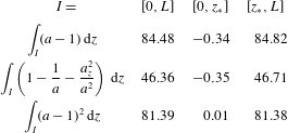
6 Comparison of modulation theory with experiment
Theory predictions for the number of solitary waves in physical experiments are reported in figure 9. We calculate the prediction  ${\mathcal{N}}$ from a smoothed version of the viscous fluid conduit’s observed profile at the time of wave breaking. Filled dots and the vertical axis in figure 9(a) report the number of observed solitary waves for each trial. We observe excellent agreement between experiment and theory, with the observed number of solitary waves being at most two away from the predicted value. Consequently, there is a decrease in the relative percentage error as the total number of solitary waves increases, as shown in figure 9(b).

Figure 9. (a) Number of solitary waves from experiment (circles) versus the number expected from (4.1). The dashed and dash-dotted lines represent one and two solitary waves away from the expected  $1:1$ relationship. (b) Percentage relative error versus the expected number of solitary waves.
Figure 10 details comparisons between asymptotic predictions and physical observations of the solitary wave amplitude c.d.f.s. The prediction from KdV analysis is included. For the amplitude distribution  ${\mathcal{F}}({\mathcal{A}})$, any relative minimum in the initial profile results in unphysical predictions. Therefore, instead of using the true profile generated from boundary control, we use an averaged version, similar to that used in numerical experiments (see the inset of figure 1). We fit the box amplitude $a_{m}$ and width $w$ by extracting these values from the experimental time, location and mean height of breaking as determined by our previously introduced inflection point criterion (Anderson et al. Reference Anderson, Maiden and Hoefer2019). The box profile is approximated by
 $$\begin{eqnarray}a_{0}(z)=\frac{a_{m}}{2}\,\text{tanh}\left(\frac{z}{2.5}\right)-\frac{a_{m}}{2}\,\text{tanh}\left(\frac{z-w}{2.5}\right),\end{eqnarray}$$
where the tanh non-dimensional width 2.5 was identified as a good fit across all reported trials to both the leading-edge transition and the final amplitude distributions. Although our analysis is explicit for sharp box profiles, we find that smoothing the box does slightly influence the smaller-amplitude soliton distribution as depicted in figure 11 (see dashed versus dash-dotted curves).

Figure 10. Cumulative distribution functions of amplitude distributions from selected experiments (solid line), with the asymptotic prediction from the conduit (dashed line) and KdV (dotted line) equations. Each step in the experimental c.d.f. corresponds to a solitary wave. Box parameters: (a) width = 20 cm ( $w=90$), $a_{m}=2$; and (b) width = 40 cm ( $w=178$), $a_{m}=4$.
We also observe a change in conduit diameter of roughly  $15\,\%$ from the bottom of the apparatus to the location of solitary wave data taking. While this does not affect ${\mathcal{N}}$, it is observed to have a profound effect on ${\mathcal{F}}({\mathcal{A}})$. To compensate for this, we use the amplitude prediction from Maiden et al. (Reference Maiden, Anderson, Franco, El and Hoefer2018) for a solitary wave on a changing background for the conduit equation. We measure error via the $\infty$-norm, as this relates to the Kolmogorov–Smirnov test for comparing c.d.f.s in statistics. Across all trials, the conduit prediction has roughly half the error as the prediction from the rescaled KdV prediction.
We also compare our results to the explicit formula (5.28) for a box. We observe in figure 11 that, as the initial condition’s width increases – corresponding to a larger number of solitary waves, therefore improving the asymptotic approximation – the observed distribution approaches the expected distribution that is independent of width.

Figure 11. Normalised c.d.f.s for solitary wave amplitudes. Experiments (stairs) compare favourably to the predictions from (5.25) for the smoothed box (dashed) and predictions from (5.29) for a pure box (dash-dotted). Colour scale corresponds to initial conditions where  $a_{m}=2$ and dimensional widths (light to dark) $25,30,35,40~\text{cm}$ corresponding to non-dimensional widths $112,134,156,178$.
Our final comparison between experiment and theory involves the spatio-temporal dataset reported in figure 2(b). Utilising the nominal measured experimental parameter values reported in the caption of that figure, we determine the length and time scalings for the conduit equation in (3.2) to be  $R_{0}/\sqrt{8\unicode[STIX]{x1D716}}=1.6~\text{mm}$ and $R_{0}/(U_{0}\sqrt{8\unicode[STIX]{x1D716}})=1.17~\text{s}$, respectively. These scalings and the measured parameters determine the initial non-dimensional box width $w=156$ and height $a_{m}=1.6$. A numerical simulation of the conduit equation with these smoothed box initial data (cf. equation (6.1)) and these scalings is shown in figure 12(a). We report the non-dimensional diameter $\sqrt{a}$ in the figure (black curves) in order to directly compare the numerics with experiment. The conduit equation simulation domain was taken to be larger (160 cm in figure 12a and 180 cm in figure 12b) than the view shown so that a portion of the initial box is outside the displayed viewing window.

Figure 12. Comparison of numerical (dark) and experimental (light) normalised conduit diameter evolution: (a) measured experimental parameters; and (b) fitted experimental parameters. In both panels, the experimental and simulation initial box height  $a_{m}=1.6$ is determined from conduit measurements and the experimental initial box width of 25 cm is obtained by the boundary control method (Anderson et al. Reference Anderson, Maiden and Hoefer2019). The experimental diameter is extracted from images in figure 2(b). (a) Measured nominal experimental parameters in the caption of figure 2 are used to determine the length $R_{0}/\sqrt{8\unicode[STIX]{x1D716}}=1.6~\text{mm}$ and time $R_{0}/(U_{0}\sqrt{8\unicode[STIX]{x1D716}})=1.17~\text{s}$ scales, and the non-dimensional box width $w=156$ for the numerical simulation. (b) Same as (a) except that the interior and exterior viscosities are fitted, determining the length $R_{0}/\sqrt{8\unicode[STIX]{x1D716}}=1.8~\text{mm}$ and time $R_{0}/(U_{0}\sqrt{8\unicode[STIX]{x1D716}})=1.13~\text{s}$ scales, and the non-dimensional box width $w=137$ for the numerical simulation.
The experimental diameter profiles  $D(Z,T)$ reported in figure 12 have been extracted from the images in figure 2(b) as per the description in § 2.2. Because of the large aspect ratio inherent in these long-wave dynamics, low image resolution in the transverse direction implies that $8~\text{pixels}\leqslant D\leqslant 20~\text{pixels}$. However, from the box and wave cameras, we have much more accurate measurements of the conduit diameter near the bottom and top of the apparatus for both the equilibrium conduit diameter (2 mm) and the diameter of the box (3.2 mm). We use these measurements to normalise the pixel data via the linear transformation $D^{\prime }(Z,T)=\unicode[STIX]{x1D6FC}D(Z,T)+\unicode[STIX]{x1D6FD}$. The coefficients $\unicode[STIX]{x1D6FC}=0.11~\text{pixel}^{-1}$ and $\unicode[STIX]{x1D6FD}=0.30$ are chosen so that the mean equilibrium conduit is $\overline{D^{\prime }}=1$ and the box diameter satisfies $D^{\prime }=3.2/2=1.6$. This normalisation effectively registers the low-resolution data in figure 2 with the high-resolution measurements from the other cameras. The profiles $D^{\prime }(Z,T)$ are reported in figure 12 with the lighter grey curves.
While the experiment gives rise to 14 solitary waves, the numerics produce 16. But the lead solitary wave diameter is only 4.5 % larger than experiment. The numerical evolutionary time scale is somewhat slower than the experimental one, which is consistent with previous measurements of large-amplitude solitary waves that were found to propagate faster than the conduit equation’s solitary wave speed–amplitude relation (2.3) predicts (Olson & Christensen Reference Olson and Christensen1986; Maiden et al. Reference Maiden, Lowman, Anderson, Schubert and Hoefer2016).
In figure 12(b), we utilise the same measured parameters as in figure 12(a), except that we fit the interior  $\unicode[STIX]{x1D707}^{(i)}=6.88\times 10^{-2}~\text{Pa}~\text{s}$ and exterior $\unicode[STIX]{x1D707}^{(e)}=0.9~\text{Pa}~\text{s}$ viscosities by increasing the non-dimensional length scale by the factor $16/14$ and reducing the non-dimensional time scale by the factor $0.97$. This particular increase in length scale derives from the predicted linear scaling of the number of solitary waves by the initial box width. Indeed, figure 12(b) exhibits precisely 14 solitary waves from both numerics (non-dimensional initial box width $w=137$) and experiment. The increased length scale and slightly reduced time scale lead to significantly improved solitary wavetrain evolution when compared with experiment. Remarkably, at the final reported time $t=177~\text{s}$, the numerical and experimental normalised diameter profiles are almost indistinguishable for the 11 largest solitary waves in the solitary wavetrain.
For the fit, the exterior viscosity is reduced by 10 %. The high-viscosity glycerine utilised for the exterior fluid is extremely sensitive to even small amounts of interior fluid mass diffusion from the conduit. A 10 % reduction from its nominal value is certainly possible. The interior viscosity’s fitted value is approximately 39 % larger than its measured value, which is a bit more than expected. However, we have not accounted for uncertainty in the volumetric flow rate or fluid densities. Moreover, the conduit equation is a long-wave approximation of the full two-fluid, free-boundary dynamics that is valid in the small-viscosity-ratio  $\unicode[STIX]{x1D716}=\unicode[STIX]{x1D707}^{(i)}/\unicode[STIX]{x1D707}^{(e)}$ regime (Lowman & Hoefer Reference Lowman and Hoefer2013a). For these experiments, the measured value of this ratio is $\unicode[STIX]{x1D716}=0.049$ and the fitted value is $\unicode[STIX]{x1D716}=0.076$. Despite these reasonably small non-dimensional values, a number of higher-order effects, e.g. inertia and the finite-sized boundary (Lowman & Hoefer Reference Lowman and Hoefer2013a), could be influencing the dynamics on the long time scales considered – the non-dimensional final time is approximately 150 in both figures 12(a) and 12(b). For these reasons, we find the comparison between experiment and the conduit equation reported in figure 12(b) to be credible, strong evidence for both the conduit equation as an accurate model of viscous fluid conduit dynamics and the efficacy of the solitary wave resolution method.
7 Conclusion
We have derived explicit formulae accurately predicting the asymptotic number and amplitude distribution of solitary waves that emerge after a long time from a localised, slowly varying initial disturbance for the conduit equation. Our analytical approach to the solitary wave fission problem is based upon Whitham modulation theory. The predictions have been quantitatively verified with experiments on the interfacial dynamics of two high-contrast viscous fluids. While the solitary wave resolution method utilised here was previously developed by El et al. (Reference El, Grimshaw and Smyth2008) for the Serre–Green–Naghdi equations modelling large-amplitude shallow-water waves, we have identified two new, universal predictions for box-shaped initial disturbances: (i) the asymptotic number of solitary waves is linearly proportional to box width; and (ii) the asymptotic normalised c.d.f. for the solitary wave amplitudes is independent of box width. Here ‘universal’ means that these predictions apply to a broad class of dispersive hydrodynamic equations (5.31), not just the conduit equation.
Our experiments are the first that validate the solitary wave resolution method and we find that the physical evolution of viscous conduit profiles is well captured by the approximation, particularly for large width disturbances. All observed solitary wave counts are within one to two waves of their expected values and within 10 % relative error for disturbances producing at least 12 waves. Amplitude distribution predictions agree quantitatively with experiment and demonstrate the necessity of going beyond the standard weakly nonlinear KdV model as it applies to the viscous fluid conduit system. The conduit’s observed, full spatio-temporal evolution exhibits remarkable fidelity to numerical simulations of the conduit equation when the two fluids’ viscosities are appropriately fitted to effectively account for a variety of uncertainties and higher-order effects in the experiment. When this work is considered in conjunction with the large variety of previous experiments on viscous fluid conduits involving solitary waves (Olson & Christensen Reference Olson and Christensen1986; Scott et al. Reference Scott, Stevenson and Whitehead1986; Whitehead & Helfrich Reference Whitehead and Helfrich1988; Helfrich & Whitehead Reference Helfrich and Whitehead1990; Lowman et al. Reference Lowman, Hoefer and El2014), wave breaking (Anderson et al. Reference Anderson, Maiden and Hoefer2019), rarefaction waves and dispersive shock waves (Maiden et al. Reference Maiden, Lowman, Anderson, Schubert and Hoefer2016, Reference Maiden, Anderson, Franco, El and Hoefer2018), the analytically tractable conduit equation and the effectiveness of Whitham modulation theory further bolster the claim that the viscous fluid conduit system provides both an ideal laboratory environment and a mathematical modelling framework in which to examine dispersive hydrodynamics and nonlinear dispersive wave dynamics more generally (Lowman & Hoefer Reference Lowman and Hoefer2013a; Maiden & Hoefer Reference Maiden and Hoefer2016).
Largely due to the paucity of analytical tools for studying strongly nonlinear wave dynamics, researchers have focused primarily on integrable models such as the KdV and modified KdV equations to obtain physical predictions for the soliton fission problem. A case in point is the field of internal ocean waves where strongly nonlinear solitary waves are known to be prevalent yet can only be explained with fully nonlinear models (Helfrich & Melville Reference Helfrich and Melville2006). Because the solitary wave resolution method is agnostic to integrable structure, a promising application direction is the fully nonlinear Miyata–Choi–Camassa (MCC) equations for two stratified fluid layers (Miyata Reference Miyata1985; Choi & Camassa Reference Choi and Camassa1999). The MCC equations have all the necessary ingredients to apply the solitary wave resolution method (Esler & Pearce Reference Esler and Pearce2011).
These results quantify an extension of the soliton resolution conjecture from integrable systems to non-integrable systems that, oftentimes, more closely model physical systems. The conjecture states that localised initial conditions to nonlinear dispersive wave equations generically evolve in long time towards a rank-ordered train of solitary waves separated from small-amplitude dispersive waves (Segur Reference Segur1973; Schuur Reference Schuur1986; Deift et al. Reference Deift, Venakides and Zhou1994). Here, we have formally derived quantitative measures of the solitary wave component, which typically dominates the long-time outcome in problems with large-scale localised initial data. Predicting properties of the accompanying small-amplitude dispersive waves is the next step towards quantifying an extension of the full conjecture to non-integrable systems.
These promising results for solitary wave fission in the model conduit system provide inspiration for future studies on this problem in other complex systems.
Acknowledgements
This work was supported by NSF DMS-1255422 and DMS-1517291 (M.A.H.), the NSF GRFP (M.D.M.), NSF EXTREEMS-QED DMS-1407340 (E.G.W.) and EPSRC grant EP/R00515X/2 (G.A.E.).


 Open access