

At the most basic level, subsistence farmers in rural Africa combine natural resources with human resources to make a living. They use mainly household labor on their own small plots to produce food for their consumption. Therefore, their household allocations of total available time to various activities has an important effect on the agricultural labor supply, production patterns, productivity, and, ultimately well-being. In households in which there are a large number of children, domestic and reproductive labor compete with agricultural labor, and mothers especially must allocate a greater amount of time to caring for children. Since women supply a substantial amount of the agricultural labor in rural Uganda (Ali et al. Reference Ali, Bowen, Deininger and Duponchel2015), their time spent caring for children and additional rest needed during pregnancy are likely to have a disproportionately negative impact on agricultural households that is quite different from the impacts of other reductions of a household's labor supply, such as illness of a male member.
Fertility rates in Uganda remain among the highest in the world even in the context of large reductions in child mortality. On average, Ugandan women in rural areas bear 6.8 children over the course of their reproductive lives (Uganda Bureau of Statistics (UBOS) 2014). At the same time, a substantial part of the population lives in rural areas and makes a living from semi-subsistence agriculture. Uganda's agriculture sector employs about 72 percent of the active labor force (UBOS 2014). Virtually all households in rural areas engage in farming, and the vast majority are small-scale, semi-subsistence farmers. Consequently, the question of how fertility affects well-being through its impact on household labor supplies and agricultural production is important.
In this study, we investigate the effect of fertility on the division of labor and agricultural production at the household level using data from a household survey conducted in Uganda. In particular, we investigate the effect of the number of biological children on households' member labor input in agriculture, which we further categorize as land preparation, weeding, input application, and harvesting. We also look at the effect of fertility on crop portfolios, area cultivated, production, and productivity for the nation's five most important crops—maize, beans, sweet potatoes, cassavas, and matookes, a starchy cooking banana. Fertility is a choice variable for agricultural households. For instance, mothers who work long hours in the field may try to avoid becoming pregnant because it would only increase their hardship. If fertility, agricultural labor allocations, and agricultural production are jointly determined, one must find a way to separate exogenous variation from variation that is jointly determined to uncover the true causal effect of fertility on the outcome variables. We use the fact that conservative, patriarchal societies such as Uganda's generally prefer male off-spring to female off-spring, resulting in particular fertility patterns (e.g., if the first three children born are girls, the family will continue to have children in hope of having boys whereas they might stop having children if the first three are boys). The random nature of a newborn's sex means that we can use reproductive patterns as an instrumental variable to determine the exogenous component of variations in fertility at the household level (Angrist and Krueger Reference Angrist and Krueger2001).
We find that the sex of the first child born, the sex of the first two children born, and the percentage of a mother's children who are girls significantly explain observed fertility, which is measured as the difference between the actual number of children born to a woman and a theoretical maximal fecundity for each age cohort; high levels of fertility are represented by small differences. We further find that greater fertility has a strong negative effect on the number of days the mother works in the field. There is evidence of a negative effect on the father as well, but the size of that effect is half of that on the mother. Households with relatively low fertility devote significantly more time than other households to land preparation and weeding. Relatively small households produce the most matooke and sweet potatoes. We find no impact of fertility on yields.
Related Studies
Fertility and the related concept of household size affect household well-being through consumption and production. Lanjouw and Ravallion (Reference Lanjouw and Ravallion1995) focused on the effects of household size on consumption in a developing country. Their results contradicted the widely held view that larger households were usually relatively poor (due to increased competition for food) and that economies of scale in consumption had little offsetting effect. When they accounted for economies of scale in households, the negative correlation between household size and consumption expenditures disappeared. On the production side of farm households, the effect of household size is equally ambiguous. Larger households theoretically have a greater supply of labor that is not subject to the effects of moral hazard often attributed to hired labor.Footnote 1 At the same time, though, a larger number of dependents in a household means that more time must be allocated to caring for them. Also, agricultural labor could be subject to diminishing returns.
The relationship between fertility and the supply of household labor has been studied most carefully in the field of labor economics in developed countries. Since this literature is so extensive, we mention only two of the most influential works here. The first is Angrist and Evans (Reference Angrist and Evans1998), which attempted to quantify the effect of fertility on labor supply in the United States. That study dealt with the endogeneity of the number of a woman's children by exploiting the American preference for having both boys and girls (Williamson Reference Williamson1976), arguing that parents of same-sex siblings were more likely to have an additional child. They also found a larger number of children in a household reduced the mother's participation in the labor force but that effect was less pronounced than found in previous studies. They found that fertility had no effect on the labor force participation by fathers.
In the second study, Rosenzweig and Wolpin (Reference Rosenzweig and Wolpin1980a), exogenous variation in the number of children was obtained using the occurrence of twins as a woman's first-born as an instrument. The authors argued that comparing women whose first child was a singleton to women whose first children were twins allowed them to identify the causal effect of an extra child on an outcome (labor supply in their case). Since the occurrence of twins was exogenous, there was no danger that heterogeneity in women's preferences influenced the estimated coefficients. They found that household size only temporarily reduced the supply of female labor.Footnote 2
In the context of developing countries, Gupta and Dubey (Reference Gupta and Dubey2006) used the sex of the first two children as a natural experiment and found that poverty increased with household size in India. They made essentially the same argument we make, but their measure of welfare and the related concept of poverty relied on consumption per capita, which, as the independent variable, is likely to be problematic in a two-stage least-squares setting. There is a real possibility that the instrumental variable will affect the outcome variable directly rather than only through its influence on family size. For instance, if boys consume more food on average than girls, the exclusion restriction would be violated. Further evidence comes from Indonesia, where Kim et al. (Reference Kim, Engelhardt, Prskawetz and Aassve2009) found that consumption decreased with an additional child. Kim and Aassve (Reference Kim and Aassve2006) related fertility to the allocation of labor in households but moved away from the direct instrumental variable approach that is standard and instead estimated a reproduction function that took endogenous contraceptive choices into account.Footnote 3
We are aware of no studies that have looked directly at the effect of fertility on agricultural labor and production decisions. However, since the bulk of the work related to bearing and rearing children falls to the women in a household, fertility is directly related to gender, and we can gain additional insights from the large body of literature on gender and agriculture. There is a well-documented gap of 20–30 percent in productivity between plots owned or managed by men versus those owned or managed by women (Udry Reference Udry1996, Food and Agriculture Organization 2011), and a number of studies have explored the reasons for it. Some studies (Agarwal Reference Agarwal1994, Lastarria-Cornhiel Reference Lastarria-Cornhiel1997, Deere and Leon Reference Deere and Leon2003) have found evidence that the lower productivity of plots managed by women can be partly explained by limits on their property rights. Several studies (Peterman, Behrman, and Quisumbing Reference Peterman, Behrman, Quisumbing, Quisumbing, Meinzen-Dick, Raney, Croppenstedt, Behrman and Peterman2014, Chen, Bhagowalia, and Shively Reference Chen, Bhagowalia and Shively2011) have attributed the gap to differences in non-land inputs and access to technology and services. In addition, women may generally have different priorities that influence their land allocations and crop mixes (Doss Reference Doss2002), and the sexual division of labor in agriculture means that labor by men and women cannot be regarded as perfect substitutes (Jacoby Reference Jacoby1991).
Peterman et al. (Reference Peterman, Quisumbing, Behrman and Nkonya2011) in a study in Uganda found persistently lower productivity for plots managed by women and for female-headed households. Ali et al. (Reference Ali, Bowen, Deininger and Duponchel2015) used panel data from Uganda and a Oaxaca decomposition and found that lower productivity on female-managed plots could be attributed to the fact that women used less fertilizer and chemicals and fewer improved seeds. Another important determinant of the productivity gap identified by the study was that women less often cultivated cash crops such as bananas and coffee. Still, about 30 percent of the productivity gap remained unexplained. Ultimately, the authors were able to attribute two-fifths of the productivity gap to women's greater childcare responsibilities, leading them to propose low-cost approaches such as community-based childcare to ease those constraints. Similar results were found by Kilic, Palacios-López, and Goldstein (Reference Kilic, Palacios-López and Goldstein.2015) in a study conducted in Malawi.
Preferences for Boys and Fertility
There is considerable evidence that parents prefer boys to girls in many developing countries.Footnote 4 Numerous studies have looked at correlations between a child's sex and variables related to well-being and health and found significant differences in outcomes attributed to sex bias. Das Gupta (Reference Das Gupta1987) and Sen (Reference Sen1990) looked at high rates of mortality among female infants in India and Chen, Huq, and D'Souza (Reference Chen, Huq and D'Souza1981) and Pande (Reference Pande2003) investigated differential access to health care for boys and girls in Bangladesh and India respectively. Behrman (Reference Behrman1988) and Hazarika (Reference Hazarika2000) found correlations between sex and nutrition and Behrman, Pollak, and Taubman (Reference Behrman, Pollak and Taubman1982), Davies and Zhang (Reference Davies and Zhang1995), and Alderman and King (Reference Alderman and King1998) all found correlations between children's gender and the education they received.
Such preferences for boys have also been directly expressed by parents in surveys. Those preferences lead to decision rules associated with fertility in which the likelihood that a household will add more children is positively correlated to the number of surviving girls in the household. Jayachandran and Kuziemko (Reference Jayachandran and Kuziemko2011) referred to such decision rules as the “stop after a son” fertility pattern. Many studies have shown empirically that parents who have just had a son are more likely than parents who just had a daughter to stop having children (Das Reference Das1987) or to wait longer to have another child (Trussell et al. Reference Trussell, Martin, Feldman, Palmore, Concepcion and Bakar1985, Arnold, Choe, and Roy Reference Arnold, Choe and Roy1998, Clark Reference Clark2000, Drèze and Murthi Reference Drèze and Murthi2001).
Jayachandran and Kuziemko (Reference Jayachandran and Kuziemko2011) argued that a preference for sons led mothers to breastfeed daughters for a relatively short time. Since breastfeeding is an effective form of birth control, this observed behavior could explain why parents of sons seemed to wait longer before having another child. This consequence of sex bias also may partly explain a range of observed outcomes in terms of health and mortality and possibly even educational attainment. The authors' model showed that disparities could arise passively because of fertility preferences even when parents wanted boys and girls to have equal health and education. The “try until you have a boy” fertility rule results in girls having more siblings on average, which leads to greater competition for resources in the household.
A preference for boys has been explained by various cultural and economic factors documented in anthropological and demographic studies. In countries in which there is no formal, risk-free insurance in old age (such as pensions), parents may choose to invest more in the children who are more likely to be able to support them in old age (Behrman, Pollak, and Taubman Reference Behrman, Pollak and Taubman1982). The anthropological and demographic evidence emphasizes the dominant role of males in traditional patrimonial societies in which descent and inheritance are transmitted through the male line. Furthermore, male children strengthen the relationship between a wife and her husband's kin by guaranteeing continuation of his lineage and secure the wife's access to an inheritance and a place to live upon her husband's death. Older women obtain power through their sons and rule over their daughters-in-law (Kandiyoti Reference Kandiyoti1988). In addition, the spread of primary schooling in sub-Saharan Africa has affected fertility patterns (Lloyd, Kaufman, and Hewett Reference Lloyd, Kaufman and Hewett2000). Because boys are more likely to be sent to (and kept in) school than girls, the extra cost in terms of lost labor associated with primary schooling is higher for families that have sons. This, in turn, encourages parents who already have boys to reduce their fertility.
Most of the evidence of the existence of preferences for sons comes from Asian countries; relatively few inquiries have been made into such preferences in sub-Saharan Africa, which was assumed to be free or nearly free of such gender preferences. This is surprising since many of the cultural and economic factors used to explain male preference in Asia apply equally to Africa. One study that has documented significant gender bias in Africa is Anderson and Ray (Reference Anderson and Ray2010), which found skewed sex ratios in favor of men in the composition of households at older ages. Another study (Eguavoen, Odiagbe, and Obetoh Reference Eguavoen, Odiagbe and Obetoh2007), which involved a small community in Nigeria, found that almost 90 percent of surveyed respondents reported a preference for sons. What is different from the Asian context is that the bias against females in sub-Sahara Africa is present at all ages.Footnote 5 Milazzo (Reference Milazzo2014) argued that gender bias is likely not found in births in Africa because high fertility is culturally valued and costs relatively little for households that rely on support from the extended family system. The preference for sons in Uganda was extensively documented in Beyeza-Kashesya et al. (Reference Beyeza-Kashesya, Neema, Ekstrom, Kaharuza, Mirembe and Kulane2010), albeit only qualitatively. The only quantitative assessment in Uganda to date is Bongaarts (Reference Bongaarts2013), which included Uganda in a study comparing 61 countries. That study found no evidence of a preference for sons, but it used information from a household survey on the desired number of boys and girls to calculate sex ratios, which could differ markedly from actual fertility behavior.
Data
We used data from the Uganda National Household Survey (UNHS) 2005–2006 obtained directly from UBOS. Although the survey was somewhat dated, we chose it because it provided much more information about agriculture than more-recent UNHS surveys (2009–2012 and 2012–2013). The 2005–2006 survey was structured with the Living Standards Measurement Study—Integrated Surveys on Agriculture (LSMS-ISA)Footnote 6 in mind and collected detailed information on a sample of almost 43,000 people in 7,500 households in Uganda.
The ideal data set would have been a sample of households in which parents planned to have no more children. The fact that we used a cross-section of households in which women were at various stages in their reproductive lives created some problems. Parents who have been together only a short time will have a smaller-than-average household size, and a household in which only one child has been born will tell little about any male/female preferences the family may have. The fact that we were working with a cross-section of households was also reflected in the average number of children overall of 3.13. In Uganda, women typically bear about seven children during their entire reproductive periods.
To address this problem, we used the difference between the maximum reproductive capacities of women in a set of age cohorts and the number of children they reported having.Footnote 7 We refer to this measure as the fertility gap. To obtain values for maximum reproductive capacity, we would have had to estimate the average age at menarche for the population and then divide that age by the periods required for pregnancy and post-pregnancy lactation infecundity. In addition, we would have had to incorporate the maternal mortality ratio as “censoring” women who, by virtue of multiple pregnancies, had a higher rate of mortality and exited from the sample. Instead, we chose to use the 95th percentile of the total fertility rate per age from the Demographic and Health Survey of Uganda done in 2011 (UBOS 2012), which provides a good approximation of the upper bound of age of fertility in the population.
We selected households in which the head of household indicated having at least one son or daughter living with them. The UNHS data did not report children who did not live with their parents, such as adult children living on their own. Thus, when the heads of households were around 30 years of age, the gap between the reported number of their children and their theoretical fertility began to increase rapidly. Furthermore, the first-born children were most likely to have left their parents and started households of their own so the oldest child in a household was not necessarily the first-born child. To overcome these problems, we restricted our sample to households in which the mother was 16 to 32 years of age. We chose 32 as the cut-off age because at this age, the mother's first-born would turn 16, which is our entry age into the sample of mothers. This restriction offered a second advantage. For some of our indirect outcome variables such as productivity, the gender of the first-born child could have a direct effect as well, threatening the validity of our identification strategy.Footnote 8 Young mothers meant that the children were relatively young also and thus were less likely to affect outcomes such as productivity directly.
One could argue that the sex of the first-born child is not particularly relevant when women bear an average of almost seven children in a lifetime. Indeed, given the high rate of fertility in Uganda, most households would have had a second child regardless of the sex of the first. This assumption is supported by Jayachandran and Kuziemko (Reference Jayachandran and Kuziemko2011), who found that differences in the duration of breastfeeding between boys and girls were largest around the family size that the household viewed as optimal, which was also the point at which a child's gender was most predictive of subsequent fertility. Therefore, we analyzed the effect of fertility using the sex of the first-born child, the sexes of the first two children, and the share of the household's children who were girls.
Descriptive Statistics
In Table 1, we report the results of the statistical analysis for the gender of the first few children born and for the share of a woman's children by gender on the number of children a woman had and fertility, which is represented by the probability that a household would have at least one more child (Prob+1) and calculated by determining the percentage of households that had more than one or two children. We find that the gender of the first one and two children and the share of female children affect fertility. In the sub-sample in which the first child was a boy, about 37 percent of households likely would have had at least one more child. When the first child was a girl, the probability of the household having another child was almost 40 percent.
Table 1. Gender and Fertility

Source: Author's calculations based on UNHS 2005–2006 data.
We also analyzed the effect of the first-born's gender on the gap between actual and theoretical fertility and found that households in which the first child was a boy had an average fertility gap of about 2.46 children. The gap was smaller, 2.26 children, when the first-born was a girl. This significant difference (p = 0.003) is consistent with the proposition that households in which the first-born child is a girl are more likely to have a relatively large number of children (conditional on the mother's age).
We next analyzed the effect of the gender of the first two children born using three cases: a boy followed by a boy, a girl followed by a boy, and a girl followed by a girl. We expected that the probability of having another child would be lowest when the first two children born were boys and highest when the first two children born were girls. The results support this hypothesis, generating probabilities of 13.2 percent when the first two children were boys, 13.4 percent when the first was a girl and the second was a boy, and 13.9 percent when the first two children were girls. The gap between actual and potential household size is also largest when the first two children are boys and smallest when the first two children are girls. Finally, we proposed the share of female children in the household as a potential continuous variable to be used in the regression analysis. At this point, we simply divided the sample into households in which half or more of the children were female and households in which less than half were female. We find that the average number of children is smaller (2.78 children) when less than half of the children are girls than when half or more are girls (2.88) and that there is a significant difference in the fertility gap (p-value 0.021). The number of children in households in which girls were the majority is closest to the theoretical maximum household size.
In this study, an important outcome variable is labor supply in agriculture, one of the prime pathways through which fertility is likely to affect productivity and well-being. The 2005–2006 UNHS records days worked on various plots reported separately for adult male and female household members. Most of Uganda has two cropping seasons—January through June and July through December—and households were interviewed twice over the course of a year—at the beginning of 2005 regarding July through December 2004 and at the end of 2005 regarding January through June 2005—to capture both. We consider only the 2004 July to December cropping season because data on labor allocations in agriculture were not available for the 2005 season.
Figure 1 shows reported time in fields for women, men, and children devoted to land preparation, input applications, weeding, and harvesting for the five crops most widely grown in Uganda. According to the data, women spent more time than men, a result mirrored by many studies of gender-differentiated time use in agriculture (e.g., Blackden and Wodon Reference Blackden and Wodon2006). Evers and Walters (Reference Evers and Walters2001), for example, found that women in Uganda supplied 80 percent of household labor time for food production, 60 percent for production of cash crops, and most labor for care of the household. The amount of child labor reported was negligible,Footnote 9 which again points to a loss of agricultural labor in the trade-off between time lost by the mother rearing children and time gained by extra hands. The short amount of time spent applying inputs is typical for Ugandan farmers, who use very limited amounts of fertilizer and other inputs. There is also some heterogeneity in the time men and women spend on different crops. For instance, women spend much more of their time cultivating sweet potatoes and somewhat more time cultivating beans than men do, suggesting some gender patterns of cropping in Uganda (Doss Reference Doss2002).
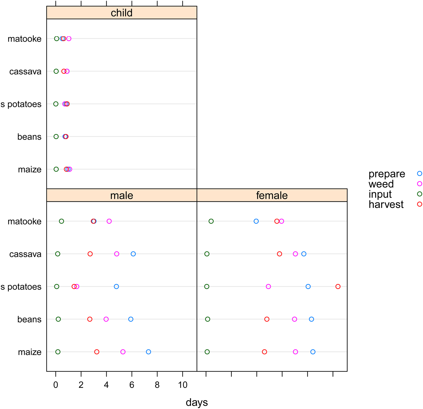
Figure 1. Average Number of Days Worked
We also investigate how fertility affects production of the five most commonly cultivated crops. Descriptive statistics on production are reported in Table 2. More than 50 percent of the households reported growing maize, beans, and cassavas. On average, households allocated about half an acre to maize and reserved the least space for sweet potatoes. In terms of area cultivated as a share of total area under cultivation, an average of about 17 percent was allocated to maize while only 8 percent was allocated to sweet potatoes. The average production of each crop in kilograms at the household level, which ranged from 128.5 for beans to 2,067.3 for matooke, is relatively low because the averages include households that did not produce the crop. We also divided by household size to calculate production per capita. Finally, we report yields per acre for the five main crops.
Table 2. Descriptive Statistics for Crop Production

Source: Author's calculations based on UNHS 2005–2006 data.
To analyze the effect of fertility on overall agricultural production, we aggregated the values of the five main crops using the average price for each crop obtained from FoodNetFootnote 10 for Kampala's Nakawa market for July through December 2004. We found that the average total value derived from the crops was about 98,500 in Ugandan shillings (UGX), which translates to about 45,000 shillings per capita.Footnote 11 About 40 percent of the households in which the adults were of reproductive age did not cultivate any of the crops. On average, farmers in Uganda allocated about 0.69 acres to the five main crops and produced an average value of 220,220 shillings per crop season.
Results
We estimate the causal impact of fertility on various agricultural outcomes using instrumental variables in a two-stage least-squares specification. The first stage regresses our proposed instruments on the fertility gap—the difference between the maximum number of children a household could have given their age and the actual number of children born. The second stage addresses the effects of fertility on agricultural labor supply, area planted, production, and productivity.
The First-Stage Regressions
Table 3 reports the results for the first-stage regressions, which link the sex of the first child/children to fertility. As previously mentioned, the dependent variable is the gap between the maximum number of children for a typical woman of a particular age and the actual number of children the women of that age bore,Footnote 12 which we refer to as the fertility gap (fgap). We further include a series of control variables that are clearly exogenous to fertility. The first, femhead, is an indicator variable that takes a value of 1 when the household head is female and 0 otherwise. The second, urban, is an indicator variable that takes a value of 1 when the household resides in an urban area and 0 otherwise.Footnote 13 Three dummy variables account for the mother's education level: mprim takes a value of 1 if the mother completed her primary education, msec represents the additional effect of the mother having completed secondary education, and mthird represents the additional effect of the mother having completed tertiary education. The comparison category, therefore, is households in which the mother did not complete primary education. We include two community variables that are likely to influence household size: school, which is a dummy variable that takes a value of 1 when there was a school in the village, and health, another dummy variable that takes a value of 1 when there was a public health center or clinic in the community. Finally, we use an indicator, cdied, that takes a value of 1 if a son or daughter of the mother had died in the past.
Table 3. First Stage Regression: Ordinary Least Square Estimation of the Fertility Gap

Note: Huber-White standard errors are shown in parentheses, and +, *, and ** denote significance at the 10 percent, 5 percent, and 1 percent level respectively.
We conducted the first-stage regressions for four alternative instruments and report the results in Table 3. In model 3-1, the excluded instrument (oldestgirl) takes a value of 1 when the first-born in the household was a girl. The estimated coefficient, –0.203, is significant at the 1 percent level and has the expected sign—when the first-born child is a girl, the fertility gap is reduced by about 0.2 children. In other words, households in which the first-born was a girl had more children on average than families in which the first-born was a boy. We also found that households headed by women had a significantly larger fertility gap of about 1.0 children. Urban households also seemed to have significantly fewer children. In terms of education, the fertility gap was slightly smaller (compared to women with no education) for women with only an elementary education and somewhat larger for women who had obtained higher levels of education. The health and school community variables did not affect fertility. Finally, the death of a child in the family led to a relatively small but significant additional fertility gap (0.284) compared to households that had not lost a child. The small magnitude of the additional gap suggests a substantial replacement effect: households that lost a child are likely to try again.
In model 3-2, the excluded instrument is an indicator variable that equals 1 when the first two children born to the mother in the household were both girls (2oldestgirls). Thus, we confine this regression to households that had at least two children, resulting in a smaller sample size. The coefficient on the excluded instrument is significantly negative, which is in line with our hypothesis, and the coefficients on the control variables are nearly identical to the estimates from model 3-1.
The regression in model 3-3 goes one step further and considers the first three children born to the mother: the excluded instrument is an indicator of households in which the first three children born were all girls (3oldestgirls). This naturally limited the size of the sample even further (N = 1,391). In this case, the coefficient is negative but is no longer significant, and we suspect that the small sample size excessively reduced the power of the t-test.
Finally, model 3-4 uses a continuous variable, the share of a household's children who are girls, as the excluded instrument (percentfemales). The coefficient on this instrument also has the expected sign: a larger share of female children in households is associated with a smaller fertility gap. This is consistent with the results of a study by Jayachandran and Kuziemko (Reference Jayachandran and Kuziemko2011), who observed that the “try until you have a boy” fertility rule led to larger households having more girls on average than smaller households. The results for the other variables are similar to the results reported in the other three models.
Overall, the results of these regressions suggest that a daughters-only household (percentfemales = 1) is, on average, 0.28 children larger than a sons-only household (percentfemales = 0).
While most of our instrumental variables are statistically significant and have expected signs, they explain only a small part of observed variances in the fertility gap. When we regressed the excluded instruments one by one on the dependent variable, the R-squares dropped below 1 percent. The F-value of a regression using only the excluded instruments, which is an important indicator of the strength of the instruments according to Bound, Jaeger, and Baker (Reference Bound, Jaeger and Baker1995), also dropped, to 9.46.Footnote 14 Thus, there was reason to believe that the instruments used in the first-stage regressions were weak and thus to use inference methods that were robust to weak instruments. In particular, we relied on the Anderson-Rubin test statistic to gauge the significance of the endogenous variable in all subsequent regressions, as suggested in Staiger and Stock (Reference Staiger and Stock1997).
Effect of Fertility on Household Labor Allocation
Table 4 shows regressions estimating the effect of fertility (measured by the fertility gap) on total time (number of days) worked in household agriculture in a year.Footnote 15 Model 4-1 reports the results of an ordinary least squares (OLS) regression that does not take endogeneity of the fertility gap into account. We find no significant correlation between the number of days worked and fertility based on the estimated fertility gap. There is a significant negative effect of women as heads of households (femhead) and households located in urban areas (urban). Primary and secondary education of mothers (mprim and msec) shows no systematic relationship to number of days worked in agriculture, but mothers who had advanced education (mthird) spent less time on agricultural work. The OLS estimates for a community school and the death of a child in the household are positively correlated with days worked by the parents. Finally, we find some evidence of a negative effect of health centers on hours worked.
Table 4. Effect of Fertility on Total Time Worked in Agriculture

Note: Huber-White standard errors are shown in parentheses, and +, *, and ** denote significance at the 10 percent, 5 percent, and 1 percent level respectively.
Models 4-2, 4-3, and 4-4 use the same general specification as 4-1 but take the endogeneity of the fertility gap into account using a single excluded instrument in two-stage least squares regressions (2SLS). In model 4-2, the instrument is an indicator that takes a value of 1 when the first-born was a girl (corresponding to first-stage model 3-1). In this case, the coefficient on the fertility gap is positive and significant at a 10 percent level, implying that greater fertility (a smaller gap) reduces the number of days parents worked on family fields. Model 4-3 uses the sex of the first-born and second-born as instruments for the fertility gap (corresponding to model 3-2) while model 4-4 uses the share of a household's children who were daughters (corresponding to model 3-4). Relative to the OLS regressions, these estimates of the effect on fertility in two-stage regressions are larger and are significant at a 1 percent level.
Model 4-5 uses both the gender of the first-born and the share of children who are daughters as excluded instruments and is estimated using limited-information maximum likelihood (LIML).Footnote 16 Based on the Hansen J-statistic, we could not reject the null hypothesis that our instruments were valid (Hansen J = 0.849, p = 0.357). In this specification, an increase in the fertility gap of one child is associated with an additional 66 days of agricultural labor by the parents. Regarding the other variables in the regression, the only significant result is a reduction in agricultural labor associated with women who have obtained an advanced education.
These results point to a substantial effect of fertility on labor time, and in an environment such as Uganda that is characterized by semi-subsistence agriculture, such a dramatic drop in time allocated to agricultural activities at the household level in response to additional children is bound to affect the household's well-being and food security. But looking only at fertility's effect on the aggregate labor supply provides limited insight into how well-being and food security are affected. We therefore conducted separate 2SLS regressions of the supply of household labor provided by adult men and by adult women in the households and report the coefficients on the fertility gap in Table 5. The regressions included the same exogenous control variables as the OLS regression.
Table 5. Two-stage Least Square Estimates of Household Labor Supply

Note: Huber-White standard errors are shown in parentheses, and +, *, and ** denote significance at the 10 percent, 5 percent, and 1 percent level respectively.
In model 5-1 (the OLS regression), the estimate of the effect of fertility on women's labor is not significant. When we account in model 5-2 for the endogeneity of fertility using exogenous variation caused by the sex of the first-born, the effect of the fertility gap is significant at a 5 percent level; an increase in the fertility gap per age cohort of one child is associated with an additional 30 days of participation in agricultural labor by women in the household. The significance of the effect of fertility on women's labor in the other models (5-3, 5-4, and 5-5) is essentially the same as in the models for agricultural labor generally. On average, an additional child is associated with a 40-day reduction in agricultural labor by women.
We next analyzed the effect of fertility on the supply of male labor in a household. As with female labor, we found that the fertility gap was not correlated with the male labor supply when we did not account for the endogenous nature of fertility choices. In the 2SLS models that accounted for the endogeneity of fertility (5-2 through 5-5), the effect of fertility on the male labor supply was less clear-cut than the effect on the female labor supply. When we used the sex of the first-born (model 5-2) and of the first two children born (model 5-3) as instruments, the coefficients were not significantly different from zero. When we used the share of all of a household's children who were female, we found that an additional child was correlated with a reduction in the male labor supply about half the size of the reduction in the female labor supply. Model 5-5 produces estimates that are significant only at the 10 percent level.
Our estimates of the effect of fertility on household labor are generally in line with the results of studies of developed countries and are particularly consistent with the results of studies of developing agricultural countries. In a study of the U.S. labor supply's response to fertility, for instance, Angrist and Evans (Reference Angrist and Evans1998) found that women worked less while men worked about the same amount of time as the number of children in the household increased, and Kim and Aassve (Reference Kim and Aassve2006) found that urban and rural Indonesian women reduced their working days in response to greater fecundity. Thus, our results provide additional support for the notion that male labor and female labor in a household are not perfect substitutes, a disparity that contributes to income inequality between men and women. It may also lead to the production inefficiencies observed for plots managed by women because women cannot devote as much time to field work (Udry Reference Udry1996). Our analysis clearly shows that increased fertility is associated with greater time poverty, which will have a detrimental effect on agricultural efforts and on the overall well-being of the household and will escalate with each additional child, presenting parents in general and women in particular (Bardasi and Wodon Reference Bardasi and Wodon2010) with difficult decisions. A larger family requires more childcare and more food while allocating additional labor to taking care of children potentially reduces the amount of food that can be produced. Women's time poverty also could restrict opportunities for education for them and their children (Arora Reference Arora2015).
Table 6 reports the results of a 2SLS regression estimating the effects of fertility on overall household labor allocations for specific types of agricultural activities: land preparations, input applications, weeding, and harvesting. Again, the table reports the estimated coefficients for the fertility gap only, but other exogenous variables from Table 4 were included in the regression. We found no significant effect of fertility on household allocation of labor in the OLS results. We thus focus mostly on the LIML results, which we deem most credible. In terms of the individual activities, an additional child reduced the time allocated to land preparation by about 25 days. None of the coefficients for input applications were significant since Ugandan households rarely use inputs such as fertilizers (see Figure 1) and spend only about one day per season planting. The only significant effect in these regressions was for households in which the mother had at least a primary school education; those households allocated more time to input applications (Van Campenhout Reference Van Campenhout2014).
Table 6. Two-stage Least Square Estimates of Household Labor Allocation

Note: Huber-White standard errors are shown in parentheses, and +, *, and ** denote significance at the 10 percent, 5 percent, and 1 percent level respectively.
The results for weeding were similar to those for land preparation but smaller in magnitude. Each additional child reduced time allocated to weeding by about 20 days. As shown in the full results in Van Campenhout (Reference Van Campenhout2014) greater fertility also had a significant negative effect on weeding in female-headed households and households in urban areas. We also found that households in communities that had a health center spent fewer days weeding.
We found no significant association between greater fertility and harvesting activities in the binary OLS regression (model 6-1). For the other regressions, the only positive effect for the fertility gap was in the model in which the exclusion instrument was the share of the household's children who were girls, and that effect was small compared to the other effects for harvesting.
These results suggest that greater fertility has a particularly negative effect on the time women allocate to land preparation and weeding (since men's allocation of time to these activities does not change significantly). Differences in time allocated to harvesting do not seem to be related to family size. Families likely must allocate most of their labor to harvesting when the crops are ripe regardless of family size. Reductions in time allocated to weeding and land preparation, on the other hand, are likely to affect yields since weeds compete for sunlight and nutrients and time-sensitive crops may not be grown or may be planted to fewer acres.
Area Planted, Production, and Productivity
Table 7 reports coefficients for the fertility gap from 2SLS regressions of planting, production, and yields for the five most important crops in the model in which the share of a household's children who are girls is the instrumental variable. These regressions include all of the control variables used in the previous models plus regional dummy variables since some crops are more prevalent in particular regions. When the dependent variable is binary or censored, we estimate a Tobit or probit model using the methods described in Newey (Reference Newey1987).
Table 7. Two-stage Least Square Estimates of Effect of Fertility on Crop Mix, Area, Production, and Yield

Note: Huber-White standard errors are shown in parentheses, and +, *, and ** denote significance at the 10 percent, 5 percent, and 1 percent level respectively. All regressions use the share of household children who are girls as the instrumental variable.
We first analyze the effect of the fertility gap on the probability that a household will grow each crop. We find that the fertility gap has no effect on cultivation of maize but is positively associated with cultivation of sweet potatoes and production of matooke. In terms of acres planted to each crop, the results show a positive association between the fertility gap and the area used to grow matooke and no association for the other crops. We considered the possibility that relatively small households that planted a large number of acres to matooke had relatively large land holdings so we analyzed the effect of fertility for the share of area planted to each crop as well. An additional benefit was the ability to evaluate the relative importance of each crop for the household. These results showed that larger households allocated a smaller share of land to sweet potatoes. In terms of kilograms of production, a smaller fertility gap (greater fertility) was associated with production of significantly less matooke, and that association persisted when we analyzed production per capita. We found no significant effect from fertility on the average yields of each crop.
Our results for planting, production, and productivity are consistent with results from Ali et al. (Reference Ali, Bowen, Deininger and Duponchel2015), which found significant differences in cropping patterns for plots managed by men versus women. Women cultivated a greater number of acres of roots, pulses, and oilseeds while men cultivated a greater number of acres of cereals, bananas, and cash crops such as coffee. In light of our results, the gender differences found by Ali et al. (2005) for bananas may be related to time constraints associated with high fertility. For roots and tubers, on the other hand, Ali et al.’s (Reference Ali, Bowen, Deininger and Duponchel2015) finding that female managers cultivated more of those crops should be attributed to factors other than fertility, such as, for example, preferences. Matooke is the only perennial crop in our analysis, and perennial crops require greater planning than annuals. In addition, Ugandans might tend to view sweet potatoes as a woman's crop given the concentration of female labor in planting them shown in Figure 1. These results are also consistent with our previous finding that fertility is negatively correlated with land preparation.
These results have significant consequences. Matooke grows in bunches that can be stored and is harvested throughout the year (about 18 months after planting). Thus, with some planning, households that cultivate matooke can have a nearly constant source of food and significant food security. Sweet potatoes are the primary source of vitamin A in Ugandan diets, and children who do not obtain enough vitamin A have a higher mortality rate because of common childhood infections such as diarrheal diseases and measles and, when the deficiency is severe, can go blind.
In a final analysis, we conducted regressions for the total productivity (yield) and value of crops produced by the household in Ugandan shillings using five models similar to the ones used in the previous analyses (Table 8). In some cases, rather than OLS, we used a probit or Tobit model that did not take heterogeneity into account (8-1) depending on the nature of the dependent variable. As before, model 8-2 used the sex of the first-born as the instrument variable, model 8-3 used the sex of the first two children born, and model 8-4 used the share of children in a household who were girls. The LIML model (8-5) used two instruments: sex of the first-born and the share of children in the household who were girls. We found no association between fertility and the total value of production for the household of the five crops. The results from the first-stage model (8-1) point to a positive association between fertility and production per capita. However, when we confined ourselves to the exogenous effect of fertility in the regressions using instrumental variables, the effect disappeared. We further found no significant associations between fertility and total crop area or productivity, which was defined as the total value of the crops divided by the total area allocated to them, and no causal impact from family size.
Table 8. Two-stage Least Square Estimates of Total Production

Note: Huber-White standard errors are shown in parentheses, and +, *, and ** denote significance at the 10 percent, 5 percent, and 1 percent level respectively.
Discussion and Conclusions
This study examines the effect of the fertility of households in Uganda on time spent working in agriculture, planting, production, and productivity by these primarily subsistence farmers. Fertility is defined as the number of biological children born to a mother. We use an identification strategy that relies on the premise that patrilineal societies such as Uganda's tend to prefer boys to girls. Thus, a household in which the first-born child is a girl is relatively more likely than a household in which the first child is a boy to have additional children (hoping to have boys). The fact that the sex of the first child born is exogenous is used to identify the causal impacts of additional children on labor supply and productivity variables. Similarly, the widely documented fertility rule in which families in patrilineal societies tend to stop having children once they have at least one boy means that households with a relatively large number of children typically have more girls than boys. Therefore, the share of children in the family who are girls can also be used as an instrumental variable. Our measure of fertility is the difference between the maximum number of children a woman in the household could bear given her age and the number of children born to the household—the “gap” in fertility; the larger the gap, the less fertile the household. We conducted a series of first-stage OLS regressions that did not take the endogeneity of fertility into account and then delved further into the effects of fertility using 2SLS regressions.
The results of our first-stage regressions point to significant negative effects on fertility when the first-born child is a girl and when the first two children born are girls. In addition, a large proportion of children in a household being girls is positively related to fertility (negatively related to the fertility gap). The coefficients from these first-stage regressions are significant and have the correct signs, but their explanatory power as measured by the partial R-square is low. We therefore use inference methods in the second-stage regressions that are robust to weak instruments.
In terms of household labor allocations and crop production, the results of our second-stage regressions suggest that fertility affected the amount of time both women and men allocated to agricultural production in general, and land preparation and weeding activities in particular suffered as the number of children in a household increased. Most of the labor time lost from an exogenous increase in children was borne by women. Of the five main crops grown in Uganda (maize, beans, sweet potatoes, cassavas, and matookes), only matooke and sweet potatoes were significantly affected by increases in fertility. Matooke is the most important staple crop in Uganda, providing 18 percent of caloric intake (Haggblade and Dewina Reference Haggblade and Dewina2010), so a reduction in matooke could have significant negative consequences for a family's food security and nutrition. Sweet potatoes provide small returns to the amount of labor required but are also a relatively resilient crop (Dercon Reference Dercon1996) and primary dietary source of vitamin A. Their production is mostly under the control of women, who do much of the work in the fields. We do not find significant effects on yields or on overall production.
Our reliance on a cross-section of households and restriction of the sample to relatively young women 16 to 32 years of age limit the extent to which our conclusions can be generalized. Couples who have a relatively large number of children might profit much more from larger households at a later stage in life. For instance, a small number of children could give a mother more time to work in agricultural activities, and children could provide inexpensive, flexible labor as they get older.
Significant policy issues are associated with fertility and its effect on households' agricultural labor and production in economies such as Uganda's. First, our analysis confirms the need for fertility-reduction policies. In addition to policies that have already shown to reduce fertility, such as education and improved health care for women, programs should identify and address the root causes of high rates of fertility. Our results show that the tendency to prefer boys to girls is one underlying cause, and there are numerous ways to change such cultural views. For example, Uganda could consider changing its laws as Kenya recently did to give equal inheritance rights to men and women. Policies should also address cultural issues related to gender roles and fertility. Some of these kinds of changes are likely to meet considerable resistance and any effort to change cultural values tends to be a very slow process. While fertility-reducing policies are being developed and implemented, the Ugandan government could provide nutritional support to young families and should consider introducing labor-saving agricultural technologies targeted to women.
Efforts to reduce fertility, including education, basic health care, and family planning, are likely to reduce time pressure for women and increase allocation of their labor to agricultural activities. Other policies could reduce the time burden associated with reproduction. For example, Uganda could established an organized system of childcare that would take advantage of economies of scale by bringing groups of children together to be cared for by one person. Technical agricultural and household innovations could focus on processes that are particularly time consuming for women, further freeing them to contribute their labor to production of food. Women are also likely to benefit from basic infrastructure improvements such as readily available clean water and local medical clinics.
It is important for any future policies and agricultural technologies to carefully consider whether the consequences of such developments affect men and women differently. For example, promoting use of oxen for preparing land for planting is likely to further increase women's time pressure, as the burden of weeding and especially harvesting falls disproportionately on women. Women must be able to use tools and technologies meant to make land preparation and weeding more efficient or effective. Equally important is providing extension and training for new technologies with women in mind. Norms and customs play significant roles in the agricultural activities performed by men and women and the norms can be highly context-specific (Deere Reference Deere1982). Efforts to change those norms and customs could affect how time is allocated to various agricultural activities by households.
The effects of fertility on production of various crops in Uganda point to specific needs by large families for greater production of crops such as matooke, which can be produced year round and withstand storage, thus potentially providing a reliable source of food. Sweet potatoes, on the other hand, provided a limited supply of food. Policies can support cultivation of matooke as well as promote smaller families.


 Open access