


Since the development and diffusion of corn hybrids in the 1930s, commercial corn yields in the United States (US) have increased dramatically over the last 80 years. Data from the US Department of Agriculture (USDA) National Agricultural Statistics Service (NASS) indicate that US corn yields have increased eight-fold from roughly 20 bu/acre in the mid-1930s to about 175 bu/acre in 2016. This tremendous growth implies a yield increase at a rate of about 1.8 bu/acre/year.
Previous literature has posited that a variety of factors, such as varietal improvement (i.e., through traditional plant breeding or genetic modification) and better agronomic practices, have contributed to this observed yield growth (Duvick Reference Duvick2005; Assefa et al. Reference Assefa, Carter, Hinds, Bhalla, Schon, Jeschke, Paszkiewicz, Smith and Ciampitti2018). However, a number of studies argue that the impressive yield increases seen in US corn can be mainly attributed to increases in planting density or plant population (i.e., the number of plants per acre) rather than to increases in per-plant yields (i.e., mainly through technological advances) (Tollenaar and Lee Reference Tollenaar and Lee2002; Tokatlidis and Koutroubas Reference Tokatlidis and Koutroubas2004; Duvick Reference Duvick2005).Footnote 1
Growth in corn plant populations in the US has roughly tracked the growth in corn yields from 1964 to 2016. In this period, yields have more than doubled, from approximately 60 to 175 bu/acre, and at the same time, plant population has also more than doubled, from about 14,000 plants/acre to close to 30,000 plants/acre. These figures suggest that yield per plant is only slightly higher in 2016 as compared to 50 years ago and therefore support the notion that corn yield growth may be largely attributed to planting density increases. However, it is likely that the link between improved corn yields and higher plant densities over time is directly influenced by increasing temperatures due to climate change, as well as varietal improvement and better agronomic practices (Lobell et al. Reference Lobell, Roberts, Schlenker, Braun, Little, Rejesus and Hammer2014; Assefa et al. Reference Assefa, Carter, Hinds, Bhalla, Schon, Jeschke, Paszkiewicz, Smith and Ciampitti2018).
The objective of this study is to determine how the yield response of corn to increasing planting density is affected by high temperatures. We are also interested in the role of genetically modified (GM) corn varieties with regard to the impact of high temperature on the “yield-planting-density” relationship. To accomplish these objectives, we utilize plot-level field trial data collected by the University of Wisconsin over the period 1990–2010 (see Shi, Chavas, and Lauer Reference Shi, Chavas and Lauer2013; Chavas and Shi Reference Chavas and Shi2015), which is then merged with publicly available weather data. Yield regression models with a variety of specifications (and interaction terms) are then estimated to understand if and how higher temperatures impact corn yield response to increasing planting density.
There is now a robust literature about corn yield response to increasing planting density, and how varietal traits and agronomic practices influence this response (see Carlone and Russell Reference Carlone and Russell1987; Porter et al. Reference Porter, Hicks, Lueschen, Ford, Warnes and Hoverstad1997; Sangoi Reference Sangoi2001; Stanger and Lauer Reference Stanger and Lauer2006; Van Roekel and Coulter Reference Van Roekel and Coulter2011; Assefa et al. Reference Assefa, Vara Prasad, Carter, Hinds, Bhalla, Schon, Jeschke, Paszkiewicz and Ciampitti2016; Lindsey and Thomison Reference Lindsey and Thomison2016; Carter et al. Reference Carter, Riha, Melkonian and Steinschneider2018; Fromme, Spivey, and Grichar Reference Fromme, Spivey and Grichar2019). For example, previous researchers, such as Coulter et al. (Reference Coulter, Nafziger, Janssen and Pedersen2010), Brown et al. (Reference Brown, Beaty, Ethredge and Hayes1970), Beech and Basinski (Reference Beech and Basinski1975), Cox (Reference Cox1996), Widdicombe and Thelen (Reference Widdicombe and Thelen2002), Nafziger (Reference Nafziger1994), Nielsen (Reference Nielsen1988), Varga et al. (Reference Varga, Svečnjak, Knežević and Grbeša2004), have examined the likely impacts of hybrids on a variety of corn agronomic responses to plant density. However, there have only been a handful of studies that specifically explored how the contribution of planting density to improved corn yields are affected by environmental factors and growing conditions.
Articles, such as Sangakkara et al. (Reference Sangakkara, Bandaranayake, Gajanayake and Stamp2004), Abbas et al. (Reference Abbas, Mascagni, Bruns, Shier and Damann2012), Brown (Reference Brown1986), Van Averbeke and Marais (Reference Van Averbeke and Marais1992), and Muchow, Sinclair, and Bennett (Reference Muchow, Sinclair and Bennett1990), have examined the impact of soil characteristics (such as soil water availability and/or soil fertility) on the relationship between corn yields and planting density. Assefa et al. (Reference Assefa, Vara Prasad, Carter, Hinds, Bhalla, Schon, Jeschke, Paszkiewicz and Ciampitti2016, Reference Assefa, Carter, Hinds, Bhalla, Schon, Jeschke, Paszkiewicz, Smith and Ciampitti2018) grouped observations into four hypothetical growth environments based on yield levels (e.g., low-yield, medium-yield, high-yield, and very high-yield environments), then estimated the corn-yield–planting density relationship for each subgroup by utilizing maximum-likelihood and least-squares-based statistical approaches. These studies found that increasing planting density has a larger positive effect on yield under a high-yield environment than a low-yield environment, which is consistent with the hypothesis in Lobell et al. (Reference Lobell, Roberts, Schlenker, Braun, Little, Rejesus and Hammer2014). In contrast, Carter et al. (Reference Carter, Riha, Melkonian and Steinschneider2018) find no evidence that higher planting density is associated with increased sensitivity to droughts (e.g., low-yield environments).
The studies of Chavas, Shi, and Lauer (Reference Chavas, Shi and Lauer2014) and Chavas and Shi (Reference Chavas and Shi2015) also investigated the effect of planting density on corn yields for different yield environments. But note that these latter two studies utilized quantile regression techniques to estimate the “yield-planting-density” function (i.e., rather than defining specific high versus low-yield subgroups and using maximum likelihood or least squares to estimate the function for each subgroup). In addition, Chavas, Shi, and Lauer (Reference Chavas, Shi and Lauer2014) and Chavas and Shi (Reference Chavas and Shi2015) also explored how GM traits influence corn yield response to increases in planting density. They found that the yield benefits of increasing planting density would be further strengthened when GM varieties are used. However, we have not found any study that looked at how temperature changes may directly affect corn yield response to higher planting density using econometric methods and long-run field trial data.
Our main contribution is that we examine the role of a specific environmental factor—temperature changes—with respect to how planting density affects corn yields. This has important implications for corn farmers, crop breeders, and other agricultural stakeholders, especially in a world with an increasingly warming climate and the need for climate change adaptation strategies. Although previous studies have explored how a “low-yield” environment generally influences corn yield response to planting density, none of these past studies have particularly investigated how increasing temperatures affect corn yield response to planting density. A better understanding of the effect of temperature on the “yield-planting-density” relationship would allow farmers to make better decisions at the start of the season (e.g., planting density and varietal choices) based on expected in-season temperatures during the growing period (Solomon, Chauhan, and Zeppa Reference Solomon, Chauhan and Zeppa2017).
In addition, understanding the interrelationships among crop yields, high temperatures, and planting density also provides further insights into an apparent puzzle in the climate change impacts literature. Previous studies have indicated that US crop yields and farm productivity are increasingly becoming more sensitive to higher temperatures (Lobell et al. Reference Lobell, Roberts, Schlenker, Braun, Little, Rejesus and Hammer2014; Ortiz-Bobea, Knippenberg, and Chambers Reference Ortiz-Bobea, Knippenberg and Chambers2018). Lobell et al. (Reference Lobell, Roberts, Schlenker, Braun, Little, Rejesus and Hammer2014) also hypothesized that the rise in planting density may be one of the main factors contributing to this increased sensitivity (though they did not prove this using observational data). To the best of our knowledge, no study has yet provided empirical evidence to show that higher planting density substantially contributes to the increased sensitivity of US crop yields to higher temperatures (i.e., mainly due to limited availability of long-term planting density data). Thus, findings from our study help address this gap in the literature.Footnote 2
The second main contribution is the exploration of whether GM traits would cause heterogeneity in the effect of high temperatures on the “yield-planting-density” relationship. We investigate the role of GM hybrids by including dummy variables for GM corn in the empirical specification (i.e., one for GM varieties with the rootworm (RW)-resistant trait and one for other GM varieties that do not include an RW-resistant trait).Footnote 3 Even though there have been previous studies that examined the “triple” inter-relationship among corn yields, planting density, and GM traits (Chavas, Shi, and Lauer Reference Chavas, Shi and Lauer2014; Chavas and Shi Reference Chavas and Shi2015), to the best of our knowledge, there have been no studies that examined the “quadruple” inter-relationship among corn yields, planting density, GM traits, and high temperatures. Hence, the present study contributes to further understanding of the so-called genotype (G), environment (E), and management (M) interactions (G × E × M) that determine crop yield outcomes (i.e., in our case, G is the GM trait, E is high temperatures, and M is the planting density choice).
Results from our study indicate that corn yield response to planting density varies with temperature, and the degree of variation with temperature is influenced by the GM traits. In general, the yield benefits of increasing planting density diminish as temperature increases. We find that the yield benefit of increasing planting density is reduced by 1.86 percent for every 1°C increase in the minimum and maximum temperatures in each month of the cropping season. But note that the diminishing yield benefits of higher planting density (in the presence of higher temperatures) are mitigated by the use of GM crop varieties, especially those with RW resistance traits.
Data sources and empirical approach
In this study, we use data from three sources: (1) annual corn field trial data collected by University of Wisconsin researchers over the period 1990–2010; (2) weather data drawn from the work of Schlenker and Roberts (Reference Schlenker and Roberts2009), which includes interpolated daily minimum and maximum temperature information for 4 km grid cells within the United States from 1950 to 2017; and (3) county-level Palmer Drought Severity Index (PDSI) data from the Centers for Disease Control and Prevention(CDC).Footnote 4
The University of Wisconsin field trial data include information about plot-level yields (measured in bushels per acre) and farming inputs applied (e.g., fertilizer and insecticides). Input use and management practices (e.g., tillage, rotation) utilized in the trial plots are similar to neighboring commercial fields and are consistent with normal agronomic recommendations (Chavas and Shi Reference Chavas and Shi2015). The management practices employed are typical of those used on corn farms practicing rainfed agriculture in the US corn belt. Fertilizer applications are based on soil type, soil moisture, and soil pH provided by a series of soil tests. Insecticide is only applied when the insect infestation level is above an action threshold (i.e., the pest density or damage level at which insecticide application is needed to prevent or reduce economic loss). Herbicide is used when it is necessary to control weed growth. The experimental design for these field trials was a randomized complete block design in which each corn hybrid variety was grown in at least three separate plots (replicates) at each site (i.e., to account for field variability). These trials were conducted over the years for the purpose of evaluating the yield performance of different corn hybrids (e.g., conventional hybrids versus various GM hybrids). Hence, these trials were not explicitly designed to assess planting density. As such, management practices are typically the same for plots in each site-year (i.e., which has implications for our empirical specifications as discussed further below). Further note that this is the same data set used in Shi, Chavas, and Lauer (Reference Shi, Chavas and Lauer2013) and Chavas and Shi (Reference Chavas and Shi2015) to mainly evaluate the production risk effects of various GM traits.
For the field trial data that span crop years 1990–2010, a total of 4,748 hybrids were tested in which 2,653 were conventional hybrids and 2,095 were GM hybrids. Some hybrids were tested in multiple locations and for multiple years. The data include 31,799 usable yield observations. However, for the present study, only 28,521 rainfed observations are utilized given the central role of temperature changes in our analysis. Summary statistics and descriptions of the field trial variables utilized in this study are provided in Table 1.
Table 1. Descriptive statistics of variables for Wisconsin data

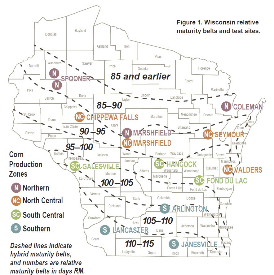
The corn field trials were conducted in 12 experimental locations (11 for rainfed corn), which are located in four production zones in the state of Wisconsin: South, South Central, North, and North Central (see Figure 1). All of the field trial locations are in what is commonly called the Northern Corn Belt. The South production zone includes three locations (or sites) in the following cities/villages: Arlington, Janesville, and Lancaster. The South Central production zone includes sites in Fond Du Lac, Galesville, and Hancock. The Chippewa Falls, Marshfield, Seymour, and Valders field trial locations are located in the North Central production zone. Lastly, the North production zone includes experimental locations in Spooner and Coleman. In general, the climatic conditions for the field trial location within a particular production zone are similar. However, it should be noted that the trial locations in the Southern production zone tend to have a more favorable climate as compared to the sites located in the other zones. The field trial locations in the South Central, North Central, and North production zones typically have a colder climate and a shorter growing season. Figures S1 and S2 show box-and-whisker plots of yield and plant density, respectively, for each of the four production zones. Notice that corn yields generally decrease as one goes further north, which is consistent with the observation that climate conditions of more southern sites are more favorable for corn. The temporal pattern of average yield and average planting density for all trial sites are presented in Figures S3 and S4. The temporal yield and planting density patterns in the data are consistent with the national trend where corn plant population growth roughly tracks the growth in corn yield.Footnote 5

Figure 1. Map of Research Locations of Wisconsin Field Experimental Data. Available at: http://corn.agronomy.wisc.edu/HT/images/Map.jpg (accessed April 7, 2019).
The grid-level weather data drawn from the work of Schlenker and Roberts (Reference Schlenker and Roberts2009) were aggregated up to the city (or village) where the field trial sites are located. After this aggregation, the monthly average daily minimum (tmin) and maximum (tmax) temperature data are then calculated. The monthly county-level PDSI data are also matched to the city (or village) where the field trial sites are located. For field trial sites wholly located in a single county, we use the PDSI value for the specific county where the trial site is located. However, for field trial sites that are on the border of two or more counties, we use a county-level average PDSI value for the corresponding counties near these trial sites. Given the nature of the weather data described above, it is important to note that all field trial plots within each site-year are assumed to have the same weather given that the tmin, tmax, and PDSI data are aggregated at the city (or village) where each field trial site is located. All weather variables are then merged with the plot-level field trial data. The summary statistics for relevant monthly minimum temperature, maximum temperature, and monthly PDSI are reported in Table 2. Moreover, the yearly changes in minimum temperatures, maximum temperatures, and PDSI for the period 1990–2010 are presented in Figures S9 and S10 for each production zone.
Table 2. Summary statistics of weather variables

Empirical specification and estimation strategies
The main empirical specification to determine how higher temperatures affect corn yield response to planting density is defined as follows:

where ln(y ilzt) is the natural log of corn yield in bushels per acre (bu/acre) for plot i, field trial location l, production zone z, and year t.Footnote 6 We estimate equation 1 using ordinary least squares (OLS) regression that includes a production zone fixed effect αz to eliminate any concerns about time-invariant unobservables at the production zone level.Footnote 7 We also include a linear time trend ηt to account for the technological improvement over time. Control variables that represent input use (or practices) are included in the vector Xilzt (e.g., fertilizer, tillage, and other variables in Table 1).
We call f( · ) in equation 1 the “weather-plant-density” function, which includes as arguments the following weather-related variables: tmin, tmax, PDSIw, and PDSId for field trial location l, production zone z, month m, and year t. Note that PDSIw refers to positive PDSI values that measure the degree of wetness (w), while PDSId refers to the absolute value of negative PDSI values that reflect the degree of dryness (d). Large PDSId values usually reflect drought conditions, and large PDSIw typically reflect extremely wet conditions (i.e., flooding).Footnote 8 The planting density variable (in ’000s of plants per acre) is also included in f( · ) and is represented by Dlzt.
In particular, the “weather-plant-density” function is defined as follows:

The growing season is specified as spanning 5-months (m = 1, 2, …, 5) from May to September. The ψ parameters associated with the interaction terms in equation 2 give us insight into how weather variables affect corn yield response to planting densities. To facilitate inference, we utilize Eicker–Huber–White (EHW) heteroskedasticity robust standard errors.Footnote 9
The specification in equations 1 and 2 is consistent with previous studies that examined crop yield effects of weather variables (see Peng et al. Reference Peng, Huang, Sheehy, Laza, Visperas, Zhong, Centeno, Khush and Cassman2004; Lobell and Field Reference Lobell and Field2007; Schlenker and Lobell Reference Schlenker and Lobell2010; Welch et al. Reference Welch, Vincent, Auffhammer, Moya, Dobermann and Dawe2010; Lobell, Schlenker, and Costa-Roberts Reference Lobell, Schlenker and Costa-Roberts2011; Tack, Barkley, and Nalley Reference Tack, Barkley and Nalley2015). These studies typically use the following variables in their specifications: tmin, tmax, and a weather variable that reflects water availability (e.g., typically quadratic functions of precipitation or rainfall). However, in contrast with these aforementioned studies, our specification above utilizes a drought index, specifically the PDSI, as a measure of water availability rather than quadratic functions of precipitation or rainfall levels.Footnote 10 A drought index like PDSI is appropriate as a measure of water/moisture availability because its values are referenced to local climate, which allows one to calculate dryness or wetness relative to local norms (Xu et al. Reference Xu, Hennessy, Sardana and Moschini2013; Kolář et al. Reference Kolář, Trnka, Brázdil and Hlavinka2014). In addition, local soil attributes are partly accounted for when calculating drought indices, which is an important factor in a crop's ability to handle extreme dryness or wetness. Using both the positive and negative PDSI values in our specification also adequately accounts for nonlinearities in the effects of water availability (i.e., typically reflected by having a quadratic precipitation term in previous studies).
Another feature of the specification in equation 2 is the linear relationship between planting density (D) and crop yields. Previous studies have typically assumed a quadratic specification for planting density (see Assefa et al. (Reference Assefa, Carter, Hinds, Bhalla, Schon, Jeschke, Paszkiewicz, Smith and Ciampitti2018) for example). However, a linear specification is appropriate in our case given that the range of our planting density data does not usually reach the reported “optimal” planting density levels recommended for Wisconsin (i.e., the yield-maximizing planting density level where corn yields plateau (the “turning point”) and consequently decreases in a quadratic specification). For example, Stanger and Lauer (Reference Stanger and Lauer2006) suggest that the optimal planting densities for Wisconsin are approximately 39,984 plants per acre for non-GM corn and 42,290 plants per acre for GM corn with the Bt trait (for the period between 2002 and 2004). Based on field trial data locations across the corn belt, Assefa et al. (Reference Assefa, Carter, Hinds, Bhalla, Schon, Jeschke, Paszkiewicz, Smith and Ciampitti2018) indicate that optimal planting density ranges from 30,500 plants per acre (in 1987) to about 37,900 plants per acre in the 2007–2016 period. In our field trial data from 1990 to 2010, the range of planting density values is from about 18,250 plants per acre to around 33,409 plants per acre. This data range is more consistent with the upward sloping (and close to linear) part of the corn yield response function to planting density, which again supports our linear specification. Furthermore, a straightforward regression of the natural log of corn yield on planting density using our data set indicates a relationship that is very close to linear and without a turning point (see Supplementary Figure S5).
Marginal effects
To achieve the study objective of assessing how the yield impact of planting density changes with temperature, we calculate the marginal effect of planting density on corn yields under different temperature scenarios based on the empirical model specified in equations 1 and 2. The marginal percentage effect of increasing plant density is the percentage change in corn yields as a result of a 1 unit (in this case, 1,000 plants per acre) increase in planting density. This marginal effect calculation can be expressed as follows:

if PDSI in each month is positive, and:

if all monthly PDSIs are negative.
In order to examine how temperature changes influence the yield response to planting density, we calculate marginal effects under two higher-temperature scenarios: (1) a scenario where both tmin and tmax change by 1°C increments, and (2) a scenario where tmin and tmax change separately by 1°C increments. To calculate the marginal effects of planting density under the first high-temperature scenario, we first assume that both the monthly tmin and tmax variables deviate from their means by the following amounts: − 1°C, − 2°C, − 3°C, − 4°C, +1°C, +2°C, +3°C, +4°C. This calculation structure allows us to see how corn yield response to planting density changes as both the minimum and maximum temperatures change (holding PDSI constant at its mean).Footnote 11 The marginal effect of planting density under the first high-temperature scenario can then be expressed as follows:

where $\xoverline [ 1.1] {\overline{\bf tmin}}_{mt}$ , $\xoverline [ 1.1] {\overline{\bf tmax}}_{mt}$
 , and $\xoverline [ 1.1] {\overline{\bf PDSI}}_{mt}$
 are set at the means in month m and year t, and the nine assumed temperature deviations are where k = −4, − 3, …, 0, …, + 3, + 4.Footnote 12
Under the second higher-temperature scenario, the marginal effects of planting density are calculated assuming that tmin and tmax separately change in 1°C increments (where k = −4, − 3, …, 0, …, + 3, + 4). The marginal effect of planting density when only tmin changes can be calculated as follows:

where tmax and the PDSIs are held at their mean values. On the other hand, the marginal effect of planting density when only tmax changes can be expressed as follows:

where tmin and the PDSIs are held at their mean values.
The marginal effect calculations above assume that changes in temperature occur in all months of the season. However, previous literature has argued that the June to August months are the critical months for corn growth. During this period, crop growth is frequently affected by environmental stresses such as high temperatures (McWilliams, Berglund, and Endres Reference McWilliams, Berglund and Endres1999). Since silking occurs in the summer time, stress conditions that happen two weeks before or after silking typically lead to substantial reductions in yield (see McWilliams, Berglund, and Endres Reference McWilliams, Berglund and Endres1999). Therefore, we also calculate the marginal effects of increasing planting density under both the scenarios described above, but only imposing changes in the temperatures for the June to August months (i.e., and where temperatures in the other months are set at their means).
Another issue of interest in this study is to determine the role of GM corn varieties, especially those that have RW-resistant traits, with regard to how corn yield responds to planting density under different high-temperature scenarios (i.e., the “quadruple” inter-relationship among corn yields, planting density, GM traits, and high temperatures). Given this interest, we modify the “weather-planting-density” function in (2) to allow for “triple” interaction terms among the planting density variable, the weather variables, and GM corn varietal dummy variables. In this case, the corn varieties in the field trial data set are categorized into three groups: conventional varieties, GM-RW hybrids, and other GM hybrids. Note that GM-RW hybrids are those varieties that have RW resistance, either as a single-trait GM crop with only RW resistance, or a “multi-stack” variety with RW resistance combined with other traits (i.e., such as a double-stack GM with combined above-ground corn borer resistance together with below-ground RW resistance). The “other GM hybrids” category includes those GM varieties with GM traits, but specifically without the RW resistance trait (e.g., single-trait Bt corn with resistance only to European corn borers).
With the GM variety categorization above, the “weather-planting-density” specification in (2) is modified as follows (to include the GM variety dummies and triple interaction terms):

where $V^r_{ilzt}$ represents the GM variety dummy variables for plot i, field trial location l, production zone z, and year t. In the specification above, conventional corn hybrids are designated as the base group (e.g., the omitted category) and V r are dummy variables that represent the two GM varietal groups, where r = 1 corresponds to the GM-RW hybrids, and r = 2 refers to the other GM hybrids. Among the 28,521 plots in the field trial data, there are 17,680 with conventional corn, 4,044 with GM-RW hybrids, and 6,797 with the other GM hybrids. The change in varietal adoption rate over time for the four production zones is shown in Figures S6, S7, and S8.
Given the “weather-planting-density” specification in equation 8, the marginal yield effect of increasing planting density for conventional corn under the first high-temperature scenario (for k = −4, − 3, .., 0, .., + 3, + 4) can then be calculated as follows:

where the weather variables are set at their mean values in all 5 months of the growing season. On the other hand, the marginal effect of increasing planting density for the GM-RW hybrids can be written as:

where the weather variables are again set at their mean values in all 5 months of the growing season. Similarly, the marginal effect of increasing planting density for the other GM hybrids can be calculated as follows:

where the weather variables are again set at their mean values in all 5 months of the growing season. Although not shown here, similar marginal effect calculations can also be computed for the second high-temperature scenario, and for the case where we only consider temperature changes in June to August months.
Estimation results and marginal effects
The main empirical model as specified in equations 1 and 2 is estimated by OLS and, in the spirit of conciseness, the parameter estimates are presented in Supplementary Table S1.Footnote 13
High-temperature effects
To determine the influence of higher temperatures on the yield effects of planting density, we calculate the marginal effects of increasing planting density under the two scenarios described in the previous section and present results in Table 3. For the first high-temperature scenario, where both tmin and tmax are assumed to change by 1°C increments, we find that the yield benefit of increasing planting density is reduced by 1.86 percent (95 percent CI [1.67, 2.05]) for every 1°C increase in the minimum and maximum temperatures in each month of the cropping season. This result suggests that the yield benefits of increasing planting density diminish in the presence of higher temperatures.
Table 3. Estimated changes in the effects of plant density on yield as a result of 1°C increase in temperatures

Notes: (1) The results here are estimated through our main specification in equations 1 and 2. (2) The first column indicates what weather variables the marginal effects of plant density are based on. The first row indicates a 1°C increase in both tmin and tmax. The second row refers to a scenario where only tmin increases by 1°C. The third row refers to a 1°C increase in tmax. (3) The second and the third column report coefficients and p-values of the changes in the marginal effects of plant density as a result of higher temperatures (both tmin and tmax increase, and tmin and tmax separately increase) where the temperature of each month of the May–September growing season increases by 1°C. The last two columns provide coefficients and p-values of the changes in the marginal effects where the temperature of each month from June to August increases by 1°C.
As described in the previous section, we also calculate the marginal effect of increasing planting density as temperature deviates from the mean by 1°C increments (see equation 5). The results of these marginal effect calculations are graphically presented in Figure 2. The mean temperature result in Figure 2 indicates that, for average weather conditions in the study area (e.g., average minimum and maximum temperatures, as well as average PDSI), increasing planting density would negatively affect corn yields (albeit by a relatively small percentage amount). Moreover, as the minimum and maximum temperatures increase relative to the mean, increasing planting density becomes more detrimental to corn yields (e.g., a 1,000 plants per acre increase in planting density results in more than 5 percent yield reduction when minimum and maximum temperatures increase by more than 3°C from the mean). On the other hand, note that increasing planting density has a positive marginal effect on yield when temperatures are lower than the mean. The diminishing marginal effect of increasing planting density in a higher-temperature environment is consistent with the idea that inter-plant competition for nutrients and resources (i.e., water) intensifies as planting density increases, and this competition escalates further when temperatures increase.

Figure 2. Marginal Percentage Effect of Plant Densities as tmin and tmax of Each Month Deviate from the Mean by 1°C Increments. Notes: The main specification in equations 1 and 2 is implemented. The Impacts are reported as the percentage change in yield. The vertical solid lines show 90 percent confidence interval.
To better contextualize the magnitudes of our estimates, we conduct a simple back-of-the-envelope calculation. First, consider the average corn yields (176.4 bu/acre) and the average planting density in the sample (28,440 plants/acre). Then, from Figure 2, we make the assumption that when tmin and tmax are at their means, increasing planting density does not change yields (i.e., there is close to zero yield impact of increasing planting density). Thus, if we increase average planting density by 1,000 plants/acre (to 29,4400) and our temperature variables remain at the mean, then yields will still be around 176.4 bu/ac. Now suppose that tmin and tmax increase by 1°C (as in our first scenario), then our findings suggest that yields will fall by 1.86 percent compared to the scenario where there are no changes in mean temperatures. In this case, yields will be around 173.11 bu/ac (= 176.4 × 0.9814) where 0.9814 = 1 − 0.0186. This suggests that when tmin and tmax increase by 1°C, increasing planting density will result in a yield reduction of about 3.29 bu/ac. This does not seem like a large reduction, but if a farmer operates 1,000 acres and corn price is at $5/bu (consistent with prices in spring 2021), this is a revenue loss of $16,450 in one cropping season. For farms with thin margins, this revenue loss from high temperatures is substantial.
Results from the second higher-temperature scenario, where we assume that tmin and tmax increase separately in 1°C increments in all months, are fairly consistent with the marginal effect estimates calculated in the first scenario described above (see Table 3). But we note that increases in tmax tend to have a larger negative impact on the yield effects of increasing planting density (as compared to the impact of increases in tmin). This suggests that increases in daytime temperatures are more likely to negatively influence yield response to increasing planting density. This result is in line with Kucharik and Serbin (Reference Kucharik and Serbin2008) where they find that tmax plays a stronger role than tmin in creating variability for Wisconsin corn.
For the case where the two higher-temperature scenarios are applied only to the critical growth months of June to August, the marginal effect estimates are still largely consistent with the results from the earlier results where increasing temperatures affect all growing season months (see Table 3 and Supplementary Figure S11). The general pattern of results in Supplementary Figure S11 is almost the same as in Figure 2. However, the magnitudes of the temperature effects are relatively smaller for the case where increasing temperatures are only felt in the June to August months.
GM traits and temperature effects
The role of GM traits is examined based on the empirical specification in equations 1 and 8. Parameter estimates for the specification that includes the GM dummy variables (and the corresponding interactions) are presented in Supplementary Table S2. Similar to the results in Supplementary Table S1, the planting density effect on corn yields is positive if GM traits and weather variables are not taken into account.
The marginal effects of increasing planting density that considers GM traits under our two increasing temperature scenarios are presented in Table 4. Results from these marginal effect calculations generally suggest that the negative effect of higher temperatures is more strongly felt for conventional corn varieties, as compared to the GM-RW hybrids and other GM hybrids. That is, the marginal yield effect of increasing planting density is more negatively affected by increasing temperatures when conventional varieties are used. Hence, the adverse effect of higher temperatures on the yield–planting-density relationship is less for GM corn in general.
Table 4. Estimated changes in the effects of plant density on yield as a result of 1°C increase in temperatures (accounting for the type of corn hybrid)

Notes: (1) The table displays coefficients and p-values of the changes in the marginal effects of plant density as a result of 1° in temperatures. The results are calculated from the estimated results of the model specification in equations 1 and 8 (the specifications including interactions among the weather, plant density, and GM varietal dummy variables). (2) The first column indicates what weather variables the marginal effects of plant density are based on. The first row of the first panel indicates a 1°C increase in both tmin and tmax. The first row of the second panel refers to a scenario where only tmin increases by 1°C. The first row of the third panel refers to a situation where only tmax increases by 1°C. (3) The second column indicates the hybrid groups: “RW” is GM hybrids expressing Bt trait for corn rootworm. “other GM” refer to GM hybrids without Bt trait for corn rootworm. (4) The third and fourth column report coefficients and p-values of the changes in marginal effects of plant density as a result of higher temperatures (both tmin and tmax increase, and tmin and tmax separately increase) where the temperature of each month of the May–September growing season increases by 1°C. The last two columns provide coefficients and p-values of the changes in marginal effects where the temperature of each month from June to August increases by 1°C.
To better visualize the role of GM traits, we graph the marginal effects of increasing planting density under the first high-temperature scenario (i.e., increasing both tmin and tmax in all months) but separating it out by the hybrid type—conventional, GM-RW, and other GM (see Figure 3). First, at the mean temperature levels, it is important to note that increasing planting density results in a negative yield impact for conventional corn yields. In contrast, for GM-RW hybrids and other GM hybrids, the marginal yield effect of increasing planting density is positive at mean temperature levels. Second, the positive marginal effect of increasing planting density is higher for GM-RW hybrids as compared to the other GM hybrids. Moreover, even at temperatures above or below the mean level, the positive marginal effect of planting density for GM-RW hybrids is still consistently larger than the other GM hybrids. Lastly, the slope of the marginal effect line for the conventional hybrids is steeper than those of the GM-RW and other GM hybrids, suggesting that the marginal effect of increasing planting density diminishes more rapidly (as temperature rises) for conventional corn, relative to the GM-RW and other GM hybrids. Overall, these results provide some evidence that the typical yield benefits of increasing planting density can be more easily maintained under high-temperature conditions if corn varieties with GM traits are used. This outcome suggests that corn varieties with GM traits (especially GM-RW hybrids) may be more efficient in utilizing nutrients and moisture even under intensified inter-plant competition due to increasing planting density and higher temperatures. Moreover, the GM trait results here support the idea that the use of GM varieties may have facilitated the increases in planting density over time.
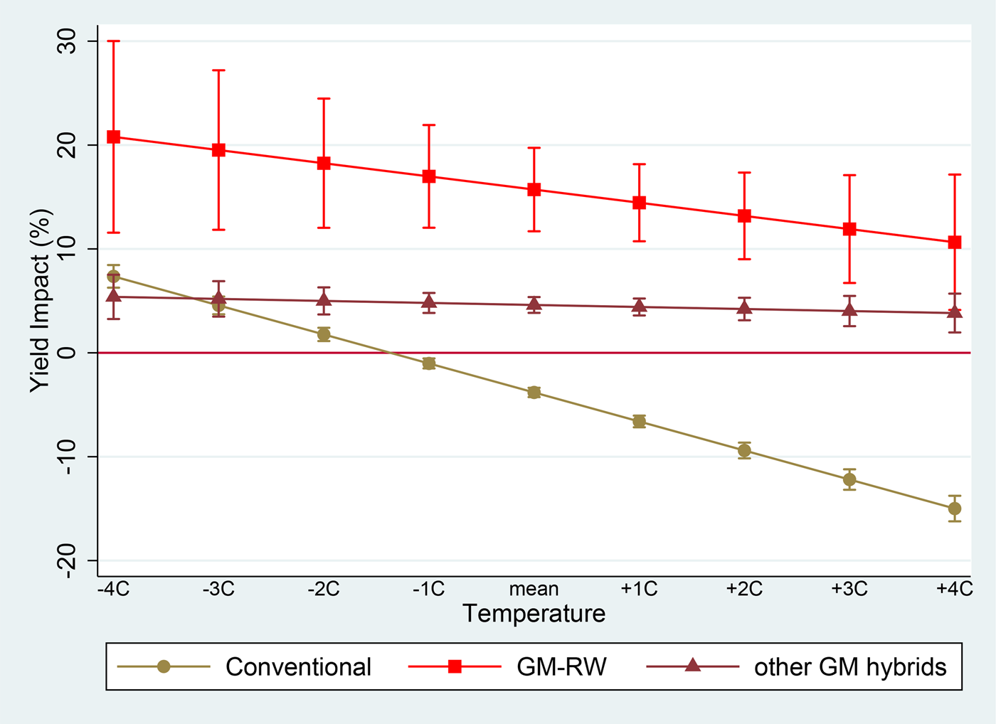
Figure 3. Marginal Impacts of Plant Density for the Three Corn Hybrid Groups, as tmin and tmax of Each Month Deviate from the Mean by 1°C Increments. Notes: The figure shows the results of the model specification in equations 1 and 8 (i.e., models including interaction terms among weather, planting density, and GM varietal group dummy variable). Impacts are reported as the percentage change in yield. The vertical solid lines show 90 percent confidence interval.
Robustness checks
To verify the strength and stability of our results, we conduct several robustness checks that consider the following alternatives to our main empirical specification (as described in equations 1 and 2): (a) the main specification without including the managerial inputs and practices (Xilzt) as control variables, (b) the main empirical specification that includes an interaction term between the time trend and the plant density, and (c) the main specification but using a quadratic form of precipitation of the May–September growing season as a measure of water availability (instead of PDSI).
We conduct the first robustness check, which excludes the managerial inputs, to account for concerns that input choices in the production process may be endogenous. However, note that this endogeneity concern may be largely mitigated by the fact the data set used in this study is based on field trial data rather than actual farm-level production data collected through a survey. Estimation results for the first robustness check are presented in Supplementary Table S3, and the corresponding marginal effects of increasing planting density for our two higher-temperature scenarios are reported in Supplementary Table S4. Supplementary Figure S12 shows the marginal percentage impact of increasing planting density for the scenario where both tmin and tmax of each month change by 1°C increments when managerial inputs are not considered in the specification. Results from this first robustness check are largely consistent with our main high-temperature results reported in the previous section. The magnitudes of the temperature effects on the corn yield response to increasing planting density are very similar to the original results above. Overall, the first robustness check still strongly supports the notion that yield effects of increasing planting density diminish as temperature levels increase.
The second robustness check aims to show whether our results still hold when one assumes that the marginal effect of increasing planting density is not constant through time. Parameter estimates for the second robustness check that include interaction terms between the time trend and planting density are presented in Supplementary Table S5, and the corresponding marginal effects are presented in Supplementary Table S6. Moreover, Supplementary Figure S13 graphically shows the marginal impacts of increasing planting density under the first high-temperature scenario in five-year increments (from 1990 to 2010). Again, the second robustness check validates our results from the main specification in the previous section. The patterns of results in Supplementary Figure S13 (for all years) are consistent with our main specification result in Figure 2. An interesting pattern to note in Supplementary Figure S13 is that the marginal yield impact of increasing planting density (for all temperature levels) shifted upward through time. This is consistent with the observation that GM adoption has increased through time, which in turn may have brought about a better yield response to increasing planting density even in higher-temperature environments (see the previous sub-section).
Then, we conduct a third robustness check where we replace PDSI as a measure of water availability with a quadratic function of precipitation (e.g., we added prec and prec 2, instead of the PDSI variables in equations 1 and 2).Footnote 14. For this last robustness check, the parameter estimates are reported in Supplementary Table S7 for the case where GM traits are not yet considered, and the corresponding marginal effects of increasing planting density for this specification are presented in Supplementary Table S8. The visual representation of the marginal planting density effects for this last robustness check (under the first high-temperature scenario) is presented in Supplementary Figure S14. All of the results for this last robustness check are fairly consistent with the direction and magnitudes of the marginal impacts of increasing planting density using the main specification. Even when we use precipitation as a measure of water availability, the marginal yield response to increasing planting density decreases when temperature levels increase.
To consider the possibility that the year effect changes over the field trial period, we run a regression using year fixed effects rather than a linear time trend in our main models. In addition, to account for a potential nonlinear plant density effect, we also run a specification that includes a quadratic plant density term into the main model. The changes in the marginal impact of plant density as a result of 1°C increase in temperatures are presented in Tables S12 and S14 and the density impacts at different temperatures estimated by these two alternative models are visually presented by Figures S16 and S17. The results from these two models are consistent with our findings in the main models above.
Parameter estimates for the specification where a quadratic form of the precipitation variable is used and GM traits are considered can be seen in Supplementary Table S9. Moreover, the marginal effects associated with this specification are presented in Supplementary Table S10. A corresponding graphical representation of the marginal effects of increasing planting density under the first higher temperature scenario, and separated out by GM type, are shown in Supplementary Figure S15. The robustness check results with precipitation used as a measure of water availability are still consistent with the results from the main specification above. At mean temperatures, the marginal effect of increasing planting density is still the strongest for GM-RW hybrids and is higher than both the conventional and other GM hybrids. At larger positive deviations from mean temperatures, this pattern still holds (as before). But note that, for mean temperatures, the marginal effect of increasing planting density for conventional corn is positive (as compared to it being negative in the main specification). In addition, the slope of the marginal effect line for conventional corn is still the steepest among the three hybrid groups. However, in contrast to the main specification results (with PDSI), the slope of the marginal effect line for GM-RW is flatter than the other GM hybrids. Nonetheless, even when precipitation is used as a measure of water availability, these robustness check results still support the notion that yield benefits of increasing planting density are better maintained under high-temperature conditions when corn varieties with GM traits are utilized.
Lastly, we conduct a robustness check where we cluster standard errors by year. This approach controls for potential spatial correlation across observations within a year (i.e., contemporaneous dependence across spatial units in a year). Regression results for this robustness check are presented in Supplementary Table S15, and the corresponding marginal effects for the main specification are in Supplementary Table S16. The marginal effects for the specification with GM interactions can also be seen in Supplementary Table S17. As expected (see footnote 9), clustering by year resulted in more conservative standard errors (relative to the case where only EHW standard errors are used) (Cameron and Miller Reference Cameron and Miller2015; Abadie et al. Reference Abadie, Athey, Imbens and Wooldridge2017). Thus, a number of parameters in the regression, as well as some of the marginal effect estimates, becomes statistically insignificant. Nevertheless, even with the more conservative standard errors, the results here are still consistent with the insights from main models. That is, the first row (and first p-value column) in Tables S16 and S17 still supports the main insight that higher temperatures reduce the yield benefits from increasing planting density. The fact that inferences from our models still hold even in the presence of more conservative standard errors speak to the robustness of our findings.
Conclusions
This study aims to explore how yield response to planting density is influenced by higher temperatures and to understand the role of GM traits in this situation. Plot-level field trial data from Wisconsin over the period 1990–2010, as well as the corresponding weather data for these field trial locations, are used to fulfill the study objectives. Yield regression models are then developed with interaction terms among planting density, weather variables, and GM hybrid dummy variables to ascertain the impact of higher temperatures and GM traits on the corn yield response to increasing planting density. Results from these models suggest that the yield benefits of increasing planting density largely diminish as temperature levels increase, and the rate of decrease is larger for conventional corn hybrids without GM traits. GM corn with RW resistance traits generally is better able to maintain the yield benefits of increasing planting density under high-temperature conditions. These results indicate that inter-plant competition for resources (e.g., nutrients and moisture) is further intensified as planting density increases and when temperatures rise, which results in diminishing benefits. But GM corn hybrids (in general) may be more efficient in utilizing these resources such that they perform better than conventional varieties even in situations with increasing planting density and higher temperatures.
Findings from the present study point to a couple of important implications. First, results from the study highlight the important role that expected growing season temperatures should play when farmers make planting density decisions and varietal choices at the start of the season. Increasing planting density does not necessarily result in yield benefits even at mean temperatures when conventional corn hybrids are used. And yield increases from higher planting density still diminish when temperatures rise. Hence, growers would likely benefit from optimizing planting density and variety choices by partly conditioning these decisions on temperature forecasts for the growing season (Solomon, Chauhan, and Zeppa Reference Solomon, Chauhan and Zeppa2017). For example, if the forecasted summer season temperature is higher than normal, then based on our results, it may be prudent to not increase planting density for conventional corn production (or only increase it slightly for GM varieties). Second, the study findings also imply that further research investments in developing corn varieties that are more tolerant to higher temperatures would likely facilitate higher optimal planting densities going forward. Not only will more heat-tolerant varieties directly reduce heat-related losses, but these types of varieties may also indirectly provide planting density-induced yield benefits. Therefore, public and private research investments for developing heat-tolerant corn varieties (i.e., either through genetic modification or traditional plant breeding) would be important to continue the trend of increasing planting density and yields into the future, especially if climate change continues to result in warmer temperatures.
Although the present study provides important insights regarding the role of higher temperatures and GM traits on the yield response to increasing planting density, there are study limitations that need to be acknowledged. First, the geographical scope of the current study is limited to the Northern corn belt and the data are from experimental field trial data rather than actual farmer data from commercial corn production. Future studies may consider using actual farm production data (i.e., data collected through farm surveys or through precision agriculture technologies) and expanding the geographical scope to more areas in the corn belt (or other locations and other corn-producing countries). Exploring the “yield-planting density” relationship in warmer climates (e.g., tropical locations) may also be beneficial. Second, the empirical analysis here would also be further improved if we had a true panel data set at the plot (or trial location) level. This would allow for using plot (or location) fixed effects and better identification of the planting density and high-temperature effects on yields. In addition, a long-term field trial data explicitly aimed to examine how planting density influences yields (e.g., field trials designed specifically to explore planting density effects (instead of variety effects) on yields) would also help in more precisely teasing out the high-temperature and GM trait effects. Lastly, having data for a longer period (i.e., more than 30 years) would also allow one to more accurately estimate long-term warming effects on the yield response to increasing planting density. We leave all these potential extensions for future work.
Supplementary material
The supplementary material for this article can be found at https://doi.org/10.1017/age.2021.10.
Acknowledgments
We would like to thank the editor, Max Melstrom, and two anonymous referees for their helpful comments and suggestions. The authors would also like to thank Guanming Shi at the University of Wisconsin for sharing the field trial data with us.
Funding statement
The work of Rejesus on this article was supported in part by USDA NIFA Hatch Project No. NC02696.
Conflict of interest
None.


 Open access