


INTRODUCTION
Many decision-making bodies process cases. Some, such as admissions committees, permitting agencies, and trial courts produce a single output for each case, a case disposition or judgment. Thus, the committee admits or rejects the applicant, the agency grants or denies the permit, and the adjudicator rules for plaintiff or defendant. Other bodies, however, produce two outputs for each case, not one. The first output remains the case disposition, but the second is a general rule or policy that rationalizes the judgment in the case. Examples of institutions that jointly produce judgments and policies include the U.S. Supreme Court, the U.S. Courts of Appeals, supreme courts and intermediate courts of appeal in the American states and some other common law jurisdictions, some high constitutional courts around the world as they engage in ex post review of statutes, and some international courts.
In this paper, we present a new model of the joint production of judgments and policies by multimember bodies like the U.S. Supreme Court. Our model of joint production captures a stylized version of procedures ubiquitous in American appellate courts and regulatory commissions both at the federal and state levels. In our formalization, the court first produces a judgment, then produces a rule that rationalizes the judgment. Members of the winning dispositional coalition bargain over the rule using procedures that we model as a sequential bargaining game. Although the model reflects American practices, the techniques employed can be adapted to study decision making on non-U.S. courts that use somewhat different practices.
We find that joint production using the American practice strongly affects policies and may affect case dispositions. First, we show that in equilibrium the median judge is pivotal over case dispositions. However, judges face an incentive to vote strategically on case dispositions in order to join the bargainers who determine policy. Equilibrium dispositional coalitions are nonetheless connected, as the most extreme judges are the least likely to vote strategically. By contrast, moderate judges, in order to affect policy, face a strong incentive to vote contrary to their preferred outcome. In particular, although the median judge is dispositionally pivotal, she may nevertheless vote strategically: the majority disposition need not always coincide with the median judge’s more preferred disposition. Case locations also affect the incentive to vote strategically on dispositions, as it is more attractive to do so when the case is close to the judge’s ideal rule cutpoint rather than far from it.
For example, Justice Kennedy, in a rare instance of candor, admitted to voting strategically on the disposition of Arizona v. Fulminante in which the Supreme Court reviewed a criminal conviction that rested on the defendant’s confession. The dispositional vote hinged on the resolution of three issues: was the defendant’s confession coerced? If it was coerced, did the harmless error rule apply? If the harmful error rule applied, was admitting the confession harmless? Justice Kennedy would have reversed the state supreme court as he believed the confession was not coerced. But he voted insincerely on the disposition, thus upholding the decision below. His strategic vote allowed him to influence the content of the opinion on the important substantive question of whether coerced confessions were subject to the harmless error rule.
Second, we show that the assigned author has considerable latitude in setting policy when bargaining is not intense (i.e., when the discount parameter δ in the sequential bargaining subgame is far from 1). In these circumstances, the opinion author, though constrained by the case location, will be able to set policy at or near her ideal policy. As bargaining becomes intense (i.e., as δ approaches 1), the dispositional majority endogenously separates into two factions. In these circumstances, the announced rule is either the ideal policy of some pivotal judge (not necessarily the median of the dispositional majority) or the result of asymmetric Nash bargaining between representative leaders of the factions, with bargaining weights proportional to faction size. Importantly, in the limit, the chosen policy never coincides with the ideal policy of the median judge of the whole court; thus while the median judge decides the disposition of the case, she does not determine the policy of the court. This result contrasts starkly with both the median voter results and median-of-the-majority results that have been proposed in the existing literature. In fact, many of the model’s predictions are new to the literature on appellate courts and regulatory commissions. Many can be tested empirically.
Reaching these results requires a contribution to the theory of sequential bargaining games. In particular, the voting rule for policy implies varying majority quotas depending on the size of the majority dispositional coalition. Consequently, we characterize the equilibria of unidimensional sequential spatial bargaining games for any super-majority quota. We further characterize the limit equilibria of such bargaining games as the discount parameter δ approaches 1. We interpret this limit as the bargaining result when the cost of proposing alternative majority opinions becomes arbitrarily small—that is, as bargaining becomes intense. We believe this situation is particularly relevant given the institutional setting of an apex court.
Literature Review
Formal models of high courts have struggled to accommodate the joint production of judgments and policy. Early models discarded judgments by treating appellate courts as “little legislatures” (Hammond, Bonneau, and Sheehan Reference Hammond, Bonneau and Sheehan2005; Jacobi Reference Jacobi2009). These models often invoked the median voter theorem, implying that opinion assignment does not affect policy. Others, responding to the wide-spread observation that majority opinions often reflect the policy views of the opinion author, invoked the Romer and Rosenthal (Reference Romer and Rosenthal1978) monopoly agenda setter model (Hammond, Bonneau, and Sheehan Reference Hammond, Bonneau and Sheehan2005). The source and limits of the opinion author’s monopoly power remained murky because any justice in the dispositional majority can offer a competing opinion and sometimes does. A second group of models discarded policy to focus on judgments, effectively treating appellate courts as “big juries” (big in the sense of singularly important; Fischman [Reference Fischman2011]; Iaryczower and Shum [Reference Iaryczower and Shum2012]; Lax [Reference Lax2007]). Despite the extremely interesting insights that follow, this approach jettisons much of what makes high appellate courts notable.
Recent papers more forthrightly address the joint production of judgments and rules. Carrubba et al. (Reference Carrubba, Friedman, Martin and Vanberg2012) stands out as particularly innovative and insightful. This paper treated judgment and policy making as a two-stage sequence and noted the importance of restricted bargaining entry. In the bargaining subgame, it focused on the core in a pure majority rule voting game within the dispositional majority, sidestepping policy consistency and the absolute-majority-in-joins rule (explained below). The model neatly rationalized the empirical finding that majority opinion location is often far from the location of the median justice of the whole Court and depends strongly on the case disposition (Clark and Lauderdale Reference Clark and Lauderdale2010). The model, however, left little room for author influence on opinion location. Nor did it address strategic dispositional voting despite the seemingly strong incentive for judges to join the dispositional majority in order to affect the bargaining outcome. Finally, preferences over judgments and policies were somewhat ad hoc.
The current paper, following Carrubba et al. (Reference Carrubba, Friedman, Martin and Vanberg2012), adapts the judgment–policy sequence and restricted bargaining entry (explained below). In addition, it explicitly addresses rule consistency, the absolute-majority-in-joins voting rule, the implications of the designated proposer procedure, and the possibility of strategic dispositional voting. The model tightly links judicial preferences over judgments and policy. These extensions allow the distinctive logic and empirical implications of the American procedure to emerge more clearly than heretofore.
THE MODEL
The American Practice
A stylized version of the American practice for jointly producing judgments and policies has the following features:
-
1. Production is sequential. The first stage is the judgment, the second policy selection.
-
2. The actors—whom we call judges—determine the judgment using pure majority rule. A minority-side dispositional vote is referred to as a “dissent.”
-
3. Judges in the dispositional majority, and only those judges, bargain over policy selection. We call this property “restricted bargaining entry.”
-
4. The policy selected by the dispositional majority must yield the judgment determined by the dispositional vote, when applied to the case. We call this property “rule consistency.”
-
5. A designated opinion author offers a policy for consideration by the dispositional majority. The judges do not modify the designated author’s proposal using a legislative-style amendment tree. Rather, each judge in the dispositional majority endorses the designated proposer’s policy (“join”) or declines to endorse the policy (“concur”).
-
6. To have precedential value, a policy must secure an absolute majority in endorsements from the full Court, not just a majority within the dispositional majority. We call this unusual voting rule “absolute-majority-in-joins.” Absolute-majority-in-joins implies that the effective voting quota in the dispositional majority depends on the majority size, and it may range from pure majority rule to unanimity.
-
7. Failure by the designated opinion author to secure an absolute-majority-in-joins may trigger another judge to propose a policy that can secure an absolute-majority-in-joins.
Actual procedures vary somewhat from institution to institution and even from case to case. Nonetheless, these seven features arguably capture the essence of the American practice. As a robustness check, we show below that weakening features (1), (3), and (5) does not significantly change the results of the model.
Cases, Dispositions and Rules
A court consisting of n judges (where n is odd) must decide a case. A case z encodes details of an event that has occurred, for example, the level of care exercised by a manufacturer or the intrusiveness of a police search. Let Z = [0, 1] be a unidimensional case space.Footnote 1 A judicial disposition d ∈ {0, 1} determines which party to the dispute prevails.
Judges dispose of cases by applying a legal rule. A legal rule r: Z → {0, 1} assigns a disposition to every potential case. We focus on an important class of legal rules, cutpoint-based doctrines, which take the following form:
 $$ r\left(z;y\right)=\left\{\begin{array}{cc}1& \mathrm{if}\hskip0.5em z>y\\ {}0& \mathrm{if}\hskip0.5em z<y\end{array}\right., $$
where y denotes the cutpoint. For example, in the context of negligence, the defendant is not liable if she exercised at least as much care as the cutpoint y. Footnote 2 Although cutpoint rules can be summarized by a threshold case, it should be clear that rules and cases are fundamentally different objects.
Decision Making by the Court
Decision making by the judges occurs in two stages. In the first stage, each judge casts a dispositional vote (dj
∈ {0, 1}) and the disposition of the court is determined by simple majority rule. The dispositional votes of each judge separate the judges into dispositional majority (denoted M ⊂ {1,..,n}) and minority coalitions. Necessarily, $ \mid M\mid \hskip1.5pt \ge \hskip1.5pt \frac{n+1}{2} $
.
$ \mid M\mid \hskip1.5pt \ge \hskip1.5pt \frac{n+1}{2} $
.
In the second stage, the justices in the dispositional majority must agree upon a legal rule y that rationalizes the chosen disposition. Consistency requires that y ≤ z if d = 1 and y ≥ z otherwise.Footnote 3 In the baseline model, we assume that once the first-stage dispositional majority is determined, it remains fixed. In Appendix A.2, we present an extension in which the judges may change their dispositional votes after observing the majority (and dissenting) opinions. With one modification, our baseline results continue to hold in this alternative setting.
The judges in the dispositional majority bargain over which legal rule to implement. We formalize this by studying a bargaining framework à la Baron and Ferejohn (Reference Baron and Ferejohn1989) and Banks and Duggan (Reference Banks and Duggan2000). Initially, a judge from the dispositional majority is recognized to propose a policy y, consistent with the majority’s disposition. Upon seeing the proposal, each judge in the dispositional majority either endorses the proposed opinion by “joining” or declines to endorse the opinion by “concurring.” To become the policy of the court, the proposal requires the assent of a majority of the entire court, not just the dispositional majority. Thus, in many cases, the dispositional majority will bargain under an effective super-majority rule.Footnote 4 If the proposal is accepted, it is implemented and the bargaining game ends. Otherwise, the process repeats itself in the following period, and this continues until the court chooses a policy. Delay within the bargaining game is costly, and the judges share a common discount factor δ ∈ [0, 1).
In the first period of bargaining, we allow the identity of the proposing judge to be nonrandom, reflecting the current practice where the most senior judge in the dispositional majority determines who will write the opinion. However, in subsequent bargaining periods, we assume judges are randomly recognized with uniform probability, reflecting the equal right of every justice to counterpropose policies.Footnote 5
Judicial Preferences
Following Carrubba et al. (Reference Carrubba, Friedman, Martin and Vanberg2012), we assume that judges’ preferences exhibit both expressive and policy components.Footnote 6 Policy utility depends on the actual policy implemented by the dispositional majority, reflecting the judge’s concern for how future cases will be decided. Expressive utility depends neither on the policy chosen nor on the actual disposition of the case, but rather, on the judge’s individual dispositional vote. Whereas policy preferences are consequentialist—they depend on actual outcomes—expressive preferences reflect the judge’s desire to be seen to decide cases “correctly,” notwithstanding, how, if at all, their vote changes actual outcomes. As will become clear, absent an expressive component of utility, judges would never have an incentive to dissent. Rather than taking an ad hoc approach to specifying these preferences, we present a framework that makes sense of both components in a cohesive way. We first specify the dispositional preferences of a given judge, and build both expressive and policy preferences from this.
Suppose judge j has ideal threshold xj and that 0 ≤ x 1 ≤ …. ≤ xn ≤ 1 so that the judges are ordered by their ideal threshold. Judge j’s dispositional utility is
 $$ {u}_D\left(d;z,{x}^j\right)=\left\{\begin{array}{ll}0\hskip2.18em & \hskip0.6em \mathrm{if}\hskip0.6em d=r\left(z;{x}^j\right)\\ {}l\left(z-{x}^j\right)& \hskip0.6em \mathrm{if}\hskip0.6em d\ne r\left(z;{x}^j\right)\end{array}\right., $$
where l(·) is a quasi-concave “loss” function that satisfies l(0) = 0 and l(·) < 0 otherwise (i.e., l has a single peak at 0). Judges face a cost when the disposition is different to their ideal. The (strict) quasi-concavity of l implies that dispositional preferences satisfy the increasing differences in dispositional values (IDID) property (see Cameron, Kornhauser, and Parameswaran Reference Cameron, Kornhauser and Parameswaran2019). This property entails that the cost of making “incorrect decisions” becomes larger the further the case is from the threshold xj. Intuitively, judges feel more strongly about “incorrectly” deciding “clear-cut” cases (those far from the threshold) than “contestable” ones (those close to the boundary separating acceptable and unacceptable conduct).Footnote 7
Expressive utility captures the judge’s desire to cast a correct vote in the current case irrespective of the rule’s influence on future cases. It is noninstrumental. It is simply the dispositional utility associated with the case outcome for which she votes, whether that outcome prevails or not. To construct policy utility, we assess the utility implications of applying rule y to decide future cases. The judge’s policy utility is her expected dispositional utility from having the next case decided according to rule y, given the distribution over cases that are likely to arise. Recall, r(z, y) is the disposition that results from applying rule y to case z. We have
 $$ {u}_P\left(y;{x}^j\right)=\int {u}_D\left(r\left(z,y\right);z,{x}^j\right) dF(z), $$
where cases are drawn from a continuous distribution F(z) with density f(z). Notice that policy utility depends on the actual chosen policy y, whereas expressive utility depends only upon the judge’s dispositional vote.
The IDID property implies that policy utility uP
(y; x) is strictly quasi-concave in y for every x, although it is not necessarily concave. Moreover, the IDID property implies that whenever xi
> xj
, $ \frac{\partial {u}_P\left(y;{x}^i\right)}{\partial y}>\frac{\partial {u}_P\left(y;{x}^j\right)}{\partial y} $
, or equivalently,
$ \frac{\partial {u}_P\left(y;{x}^i\right)}{\partial y}>\frac{\partial {u}_P\left(y;{x}^j\right)}{\partial y} $
, or equivalently, $ \frac{\partial^2{u}_P\left(y,x\right)}{\partial x\partial y}>0 $
.Footnote
8
Therefore, preferences exhibit the single-crossing property; the benefit from marginally increasing the policy y is monotone in the judges’ ideal policies.
$ \frac{\partial^2{u}_P\left(y,x\right)}{\partial x\partial y}>0 $
.Footnote
8
Therefore, preferences exhibit the single-crossing property; the benefit from marginally increasing the policy y is monotone in the judges’ ideal policies.
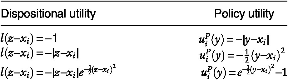
Example 1. Suppose cases are uniformly distributed on [0,1]. Table 1 provides a mapping between the dispositional loss function l and commonly used policy utility functions, including absolute-value utility, quadratic utility, and bell-curve shaped (Gaussian density) utility. Bell-curve shaped policy utility has some nice properties that we exploit in later examples.
TABLE 1. Relationship between Dispositional and Policy Utility
During the bargaining game, the disagreement payoff to each judge is uP (D; x). We make the standard assumption that disagreement is worse for each judge than agreeing to any feasible policy (i.e., uP (D, x) ≤ uP (y, x) ∀ y ∈ [0, 1]).
Overall utility is the sum of policy and expressive components:
 $$ {u}_P\left(y;{x}^j\right)+\alpha {u}_D\left({d}^j;z,{x}^j\right), $$
where α > 0 denotes the relative importance of the expressive component.
We should note the role of the “legal status quo” within the bargaining game. We take the view that any prior legal policy effectively reverts to a null policy when the Court takes the case—policy is in limbo until the Court resolves the case. Indeed, our bargaining protocol requires that bargaining continue until a majority chooses a policy. Policy may only revert to the status quo ante if the Court reenacts it anew. In Appendix A.1, we consider an alternative framework in which policy reverts to the status quo ante if bargaining fails. Our results continue to hold under this alternative formulation, and so the question of the “legal status quo” is not crucial to our analysis.
Additionally, we note that our formulation implicitly assumes that the court can commit to implementing its chosen policy when deciding future cases—that is, the announced policy is time-consistent and renegotiation-proof. Few models of collegial courts address the problem of commitment (but see Baker and Mezzetti [Reference Baker and Mezzetti2012] and Cameron, Kornhauser, and Parameswaran [Reference Cameron, Kornhauser and Parameswaran2019]). Recent legislative models of sequential policy making with evolving status quos are suggestive (Kalandrakis Reference Kalandrakis2010), but we do not pursue this point any further.
Strategies and Equilibrium
We analyze equilibrium in the policy-making stage and the dispositional-voting (adjudication) stage, in turn. Given the repeated game structure of bargaining in the policy-making stage, strategies can be quite complex because they may be history dependent. We restrict attention to stationary strategies, which require that players choose equivalent strategies in every structurally equivalent subgame. A strategy for judge j (in the dispositional majority) in the policy-making stage is a pair (yj , Aj ), where
-
• yj (z, M, δ) denotes the policy proposed whenever the judge is recognized to make a proposal, given case z and dispositional majority M ⊂ {1,..,n}.
-
• Aj (z, M, δ) denotes the set of proposals that the judge will accept, whenever she is in the dispositional majority.
The equilibrium concept is stationary subgame perfection with weakly undominated strategies. Weak undominance requires that each judge vote for her more preferred option (regardless of whether her vote would sway the outcome or not). This rules out equilibria in which judges vote for less favored outcomes, sustained by the belief that their vote will be inconsequential.
A strategy for judge j at the adjudication stage is a dispositional choice dj (z; α, δ) ∈ {0, 1} given case z, anticipating the equilibrium rule that will be chosen in the policy-making stage. An adjudication (Nash) equilibrium is a pair (d, M) denoting the majority disposition and the composition of the dispositional majority, having the property that no judge could do better by switching her dispositional vote.
THE POLICY STAGE
In this section we characterize behavior in the policy-making stage for a generic dispositional majority. In the next section, we find the optimal majority dispositional coalition, given the anticipated policy bargaining. We begin by characterizing equilibrium proposals when δ < 1. As we will see, there will be a range of policies proposed in equilibrium, reflecting the agenda-setting prerogative of the opinion author. Our approach is, thus, distinct from median-voter-type models that predict a single equilibrium policy. We subsequently reconcile the two approaches by taking the limit as the agenda-setter’s power goes to zero. Even in this scenario, the equilibrium policy will not generically coincide with the median judge’s ideal.
Equilibrium Characterization
Let z be the case, and suppose the dispositional majority coalition M ⊆ {1,…,n} contains m ∈ {k,…,n} members, where $ k=\frac{n+1}{2} $
. Without confusion, we relabel the judges in the coalition, preserving the ordering of ideal policies, so that M = {1, …, m} with x
1 ≤ …. ≤ xm. Given the two-stage structure, once the majority coalition forms, the preferences of the nonmajority judges become inconsequential to policy making, so we are free to disregard them and focus on the m remaining judges. Similarly, we may focus solely on policy utility, as the dispositional votes determine dispositional utility.
$ k=\frac{n+1}{2} $
. Without confusion, we relabel the judges in the coalition, preserving the ordering of ideal policies, so that M = {1, …, m} with x
1 ≤ …. ≤ xm. Given the two-stage structure, once the majority coalition forms, the preferences of the nonmajority judges become inconsequential to policy making, so we are free to disregard them and focus on the m remaining judges. Similarly, we may focus solely on policy utility, as the dispositional votes determine dispositional utility.
Recall that policy must be consistent with the disposition of the court. If the majority disposition was 1, the majority must choose a policy in the interval [0, z], whereas if the disposition was 0, the coalition must choose a policy in the interval [z, 1]. Generically, $ \left[\underline{x},\overline{x}\right] $
must contain the court’s policy, where
$ \left[\underline{x},\overline{x}\right] $
must contain the court’s policy, where $ \underline{x}\hskip1.5pt \in \hskip1.5pt \left\{0,z\right\} $
and
$ \underline{x}\hskip1.5pt \in \hskip1.5pt \left\{0,z\right\} $
and $ \overline{x}\hskip1.5pt \in \hskip1.5pt \left\{z,1\right\} $
.
$ \overline{x}\hskip1.5pt \in \hskip1.5pt \left\{z,1\right\} $
.
Our bargaining framework is similar to those studied by Banks and Duggan (Reference Banks and Duggan2000), Cardona and Ponsati (Reference Cardona and Ponsati2011), and Parameswaran and Murray (Reference Parameswaran and Murray2019). Because those papers provide detailed expositions of the equilibrium characterization, we defer to them and instead provide a brief intuitive account of the equilibrium. We begin by noting two important details. First, each judge bases her decision on whether to support a proposal by comparing the policy utility from the current proposal to her (discounted) expected policy utility from entertaining counterproposals. The set of equilibrium counterproposals, thus, establishes the opportunity cost of accepting a given proposal, which in turn establishes the set of proposals acceptable to each judge. Since each proposer seeks to build a winning coalition around their proposal, the anticipation of future counterproposals disciplines each judge’s decision about which policy to propose when they are recognized.
Second, because policy preferences satisfy the single-crossing property, in equilibrium, the policy coalitions that support and reject any proposal will both be connected. We stress that this is an equilibrium phenomenon; the decision rule does not require that the “join” and “concur” coalitions be connected, but optimal behavior, nevertheless, ensures that they will. Since the proposer only needs the support of $ k=\frac{n+1}{2} $
judges, it suffices to earn either the support of the left-most k judges {1,…,k} in the dispositional majority or the right-most k judges {m – k + 1,…,m}, where judge m − k + 1 is the k
th judge from the right. It follows that judges {m – k + 1,…,k} must be in every equilibrium coalition. Indeed, judges m − k + 1 and k are decisive in the sense that, in equilibrium, a proposal is winning if and only if it has both their support. Following Compte and Jehiel (Reference Compte and Jehiel2010), we refer to these as the left- and right-decisive judges, respectively. If m = n, so that the join coalition need only be a simple majority of the dispositional majority, then the left- and right-decisive judges will both coincide with the median judge. By contrast, for any m < n, m − k + 1 < k, and so, generically, the decisive judges will be nonmedian players, with distinct preferences.
$ k=\frac{n+1}{2} $
judges, it suffices to earn either the support of the left-most k judges {1,…,k} in the dispositional majority or the right-most k judges {m – k + 1,…,m}, where judge m − k + 1 is the k
th judge from the right. It follows that judges {m – k + 1,…,k} must be in every equilibrium coalition. Indeed, judges m − k + 1 and k are decisive in the sense that, in equilibrium, a proposal is winning if and only if it has both their support. Following Compte and Jehiel (Reference Compte and Jehiel2010), we refer to these as the left- and right-decisive judges, respectively. If m = n, so that the join coalition need only be a simple majority of the dispositional majority, then the left- and right-decisive judges will both coincide with the median judge. By contrast, for any m < n, m − k + 1 < k, and so, generically, the decisive judges will be nonmedian players, with distinct preferences.
For notational convenience, we index the left and right decisive judges by l and r, where l = m − k + 1 and r = k. We have the following result, which is similar (despite some important differences) to results previously noted by Cho and Duggan (Reference Cho and Duggan2003), Cardona and Ponsati (Reference Cardona and Ponsati2011), and Parameswaran and Murray (Reference Parameswaran and Murray2019), among others:
Proposition 1.
For δ < 1, the bargaining game admits a unique equilibrium. The equilibrium is in no-delay, and it is characterized by a pair $ (\underline{y},\overline{y}) $
, with
$ (\underline{y},\overline{y}) $
, with $ \underline{x}\hskip1.5pt \le \hskip1.5pt \underline{y}<\overline{y}\hskip1.5pt \le \hskip1.5pt \overline{x} $
, such that
$ \underline{x}\hskip1.5pt \le \hskip1.5pt \underline{y}<\overline{y}\hskip1.5pt \le \hskip1.5pt \overline{x} $
, such that
-
1. When recognized, judge j will propose $ {y}^j=\left\{\begin{array}{cc}\underline{y}& \hskip0.2em {x}^j<\underline{y}\\ {}{x}^j& \hskip0.2em {x}^j\in \left[\underline{y},\overline{y}\right]\\ {}\overline{y}& \hskip0.2em {x}^j>\overline{y}\end{array}\right. $
.
$ {y}^j=\left\{\begin{array}{cc}\underline{y}& \hskip0.2em {x}^j<\underline{y}\\ {}{x}^j& \hskip0.2em {x}^j\in \left[\underline{y},\overline{y}\right]\\ {}\overline{y}& \hskip0.2em {x}^j>\overline{y}\end{array}\right. $
.
-
2. The pair
$ (\underline{y},\overline{y}) $
satisfies


-
•
$ \underline{y}=\min \left\{y\hskip1.5pt \ge \hskip1.5pt \underline{x}|{u}_P\left(y;{x}^r\right)\hskip1.5pt \ge \hskip1.5pt \left(1-\delta \right){u}_P\left(D,{x}^r\right)\hskip3.55pc +\frac{\delta }{m}{\sum}_j\hskip1.5pt {u}_P\left({y}^j,{x}^r\right)\right\} $
and -
•
$ \overline{y}=\max \left\{y\hskip1.5pt \le \hskip1.5pt \overline{x}|{u}_P\left(y;{x}^l\right)\hskip1.5pt \ge \hskip1.5pt \left(1-\delta \right){u}_P\left(D,{x}^l\right)\hskip3.55pc +\frac{\delta }{m}{\sum}_j\hskip1.5pt {u}_P\left({y}^j,{x}^l\right)\right\} $
.


Proposition 1 shows that our bargaining game admits a unique equilibrium characterized by an interval $ [\underline{y},\overline{y}\} $
of “socially acceptable” policies (i.e., which will receive the support of at least k agents). In equilibrium, the proposer will offer the socially acceptable policy closest to her ideal. Judges with “moderate” preferences (whose ideal policies lie within the interval) will successfully implement their ideal rule in equilibrium, whereas judges with “extreme” preferences must offer a compromise rule. All “extreme left” judges will pool on the same proposal
$ [\underline{y},\overline{y}\} $
of “socially acceptable” policies (i.e., which will receive the support of at least k agents). In equilibrium, the proposer will offer the socially acceptable policy closest to her ideal. Judges with “moderate” preferences (whose ideal policies lie within the interval) will successfully implement their ideal rule in equilibrium, whereas judges with “extreme” preferences must offer a compromise rule. All “extreme left” judges will pool on the same proposal $ \underline{y} $
, whereas all “extreme right” judges will pool on the same proposal
$ \underline{y} $
, whereas all “extreme right” judges will pool on the same proposal $ \overline{y} $
. What constitutes “moderate” and “extreme” is itself determined in equilibrium, and it depends on the discount factor δ and the preferences of the left- and right-decisive judges. The value
$ \overline{y} $
. What constitutes “moderate” and “extreme” is itself determined in equilibrium, and it depends on the discount factor δ and the preferences of the left- and right-decisive judges. The value $ \overline{y} $
is the highest policy that the left-decisive judge is willing to accept, given her continuation payoff. Similarly,
$ \overline{y} $
is the highest policy that the left-decisive judge is willing to accept, given her continuation payoff. Similarly, $ \underline{y} $
is the lowest policy that the right-decisive judge is willing to accept. Any proposal in the region
$ \underline{y} $
is the lowest policy that the right-decisive judge is willing to accept. Any proposal in the region $ \left[\underline{y},\overline{y}\right] $
is equilibrium consistent.
$ \left[\underline{y},\overline{y}\right] $
is equilibrium consistent.
To make sense of Proposition 1, let E[y] = ∑ j pjyj be the expected policy that will be proposed (and accepted) in the continuation game. As we show in Appendix B, if E[y] is proposed, it will receive unanimous support.Footnote 9 Take a judge j in the dispositional majority whose ideal policy lies below E[y]. Since delay is costly (δ < 1), judge j can offer a policy slightly below E[y] and still retain unanimous support. Decreasing the offer further, she will eventually lose the support of the right-most judge, then the second-most-right judge, and so on. Since it suffices to have the support of the right-decisive judge, judge j will continue decreasing the offer until either she reaches her ideal policy, or the support of the right decisive judge would be lost. Thus, the preferences of the right-decisive judge pin down the lowest socially acceptable policy. Similarly, the preferences of the left-decisive judge determine the highest acceptable policy.
Example 2. Consider a case z = 0.45, and suppose the court’s disposition is d = 1. Consistency requires that y ≤ 0.45. Suppose there are six judges in the majority, with ideal policies x 1 = 0, x 2 = 0.2, x 3 = 0.25, x 4 = 0.3, x 5 = 0.4, and x 6 = 0.6. Judges 1,..,5 (and presumably the three dissenting judges) cast sincere dispositional votes, whereas judge 6 voted strategically. Since policy making requires a majority of the entire bench, k = 5. The left- and right-decisive judges, then, are judges 2 and 5, respectively. Suppose policy utility is given by uP (y, x) = −|y − x| and the common disagreement payoff is −1. Figure 1 depicts the set of socially acceptable policies for two values of δ.
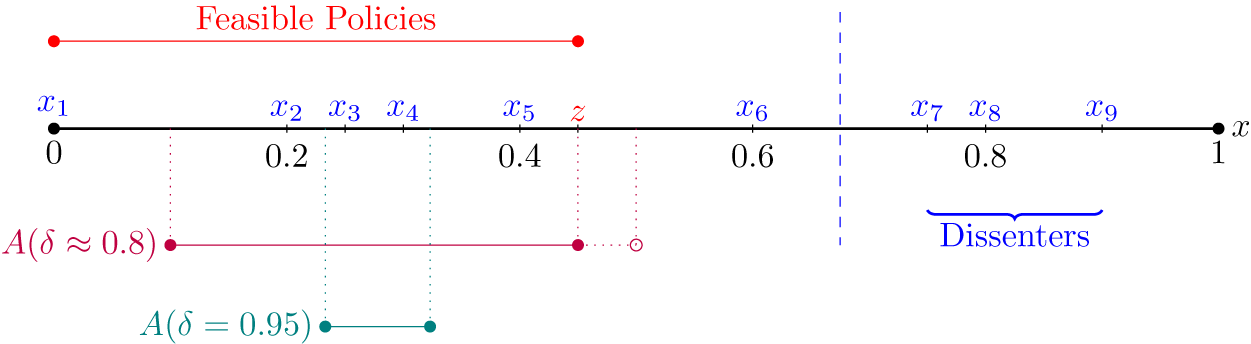
FIGURE 1. Equilibrium Socially Acceptable Policies in Example 2
Note: A(δ) represents the social acceptance set given a cost of delay δ. When $ \delta =\frac{21}{26}\hskip1.5pt \approx \hskip1.5pt 0.8 $
, A = [0.1, 0.45], whereas if δ = 0.95, then A = [0.2334, 0.3234]. Notice that when δ ≈ 0.8, the consistency constraint (i.e, y ≤ z) is binding. The dotted extension to A(δ ≈ 0.8) represents the additional policies that would be socially acceptable absent the consistency constraint.
$ \delta =\frac{21}{26}\hskip1.5pt \approx \hskip1.5pt 0.8 $
, A = [0.1, 0.45], whereas if δ = 0.95, then A = [0.2334, 0.3234]. Notice that when δ ≈ 0.8, the consistency constraint (i.e, y ≤ z) is binding. The dotted extension to A(δ ≈ 0.8) represents the additional policies that would be socially acceptable absent the consistency constraint.
In the first scenario ( $ \delta =\frac{21}{26} $
), judges 2,3,4, and 5 are able to propose their ideal policies in equilibrium, whereas judge 1 must propose a compromise policy—that is, the lowest policy acceptable to the right-decisive judge. It is infeasible for judge 6 to propose her ideal policy, and in equilibrium, she will propose the highest policy that is feasible y = 0.45. In fact, the left-decisive judge would in principle accept policies up to y ≈ 0.5; however, any policy above y = 0.45 would not rationalize the case disposition. In the second scenario (δ = 0.95), judges 3 and 4 are able to propose their ideal policies in equilibrium, whereas the remaining judges must propose compromise policies. □
$ \delta =\frac{21}{26} $
), judges 2,3,4, and 5 are able to propose their ideal policies in equilibrium, whereas judge 1 must propose a compromise policy—that is, the lowest policy acceptable to the right-decisive judge. It is infeasible for judge 6 to propose her ideal policy, and in equilibrium, she will propose the highest policy that is feasible y = 0.45. In fact, the left-decisive judge would in principle accept policies up to y ≈ 0.5; however, any policy above y = 0.45 would not rationalize the case disposition. In the second scenario (δ = 0.95), judges 3 and 4 are able to propose their ideal policies in equilibrium, whereas the remaining judges must propose compromise policies. □
Example 2 demonstrates the essential features of the equilibrium. There is a range of policies that are potentially proposed in equilibrium. Moderate judges may propose their ideal policies, whereas extreme judges (in particular, judges who vote insincerely) must propose compromise rules. Whether a judge is moderate or extreme depends on the preferences and degree of patience of the left- and right-decisive judges. Moreover, the social acceptance set may be constrained by the facts of the case itself; the consistency requirement may be binding.
Comparative Statics on δ
The discount rate δ parameterizes the cost of delay in bargaining, or (equivalently) the relative importance of the legal issue. As Example 2 demonstrates, it also represents measures of the proposer’s degree of agenda control. When δ = 0, delay is exceedingly costly relative to the importance to each judge of implementing desirable policies, so the nonproposing judges will accept any feasible policy. The proposer thus has complete control over the agenda and will propose the feasible policy closest to her ideal. Lemma 1 shows that, as δ → 1, the reverse becomes true; delay becomes costless relative to the importance of deciding the legal question correctly. The judges will bargain “aggressively” over policy such that, in equilibrium, the proposer loses control of the agenda entirely and all judges will make the same proposal. Thus, δ parameterizes the proposer’s degree of agenda control.
Lemma 1.
In any equilibrium, $ \overline{y}\left(\delta \right)>\underline{y}\left(\delta \right) $
whenever δ < 1. Moreover, there exists μ such that
$ \overline{y}\left(\delta \right)>\underline{y}\left(\delta \right) $
whenever δ < 1. Moreover, there exists μ such that $ {\lim}_{\delta\,\to \hskip1.0pt 1}\overline{y}\left(\delta \right)=\mu ={\lim}_{\delta\,\to \hskip1.0pt 1}\underline{y}\left(\delta \right) $
.
$ {\lim}_{\delta\,\to \hskip1.0pt 1}\overline{y}\left(\delta \right)=\mu ={\lim}_{\delta\,\to \hskip1.0pt 1}\underline{y}\left(\delta \right) $
.
Taken together, Proposition 1 and Lemma 1 make strong predictions about the size and composition of the “join” and “concur” coalitions. When delta is low, the cost of entertaining counterproposals is sufficiently high that all judges will support the opinion of the court. The join coalition will consist of all judges in the dispositional majority, and no judge will concur. By contrast, as δ → 1 judges become more demanding about the set of opinions that they will join. The size of the join coalition will fall to a bare majority, consisting of either the left-most or right-most k judges. In either case, the concur coalition will consist of judges from only one extreme (within the dispositional majority). Thus, regardless of the size of δ, an “ends-against-the-middle” dynamic should never arise in which the join coalition consists of relatively moderate judges and extremists from both ends concur.
Limit Equilibria and “Median Voter” Logic
Equilibrium policy making by the Court is (generically) characterized by a menu of proposer-dependent policies. Proposer dependency arises whenever it is costly for judges to make (or entertain) counterproposals. Our approach, thus, stands in contrast to many existing studies that predict a unique policy outcome, typically by appealing to median voter logic. However, as δ → 1, all judges propose a unique policy. Taking this limit, then, allows for fair comparisons between our model and those existing in the literature.
There is a tight connection between median-voter-type logic (or, more generally, the equilibrium concept of the core) and the limit equilibria of our bargaining game. For example, Cho and Duggan (Reference Cho and Duggan2009) show that when agreement requires a simple majority, the limit equilibrium policy precisely coincides with the median agent’s ideal policy. The intuition is straightforward: the logic of the median voter theorem is that, whenever a policy other than the median voter’s ideal is proposed, a majority coalition can be found that would replace it with something closer to the median voter’s ideal. This is true in our bargaining game as well, except that, when delay is costly, a non-core policy might persist, because it is too costly to make the counterproposal that replaces it. As delay become costless, this friction disappears, and so the outcome of bargaining should coincide with the median voter’s ideal.
When agreement requires a super-majority, logic analogous to the median voter theorem predicts an equilibrium outcome in the core.Footnote 10 However, under super-majority rule, the core generically contains many policies. In fact, the core is precisely the interval of policies bounded by the ideal policies of the left and right decisive voters. Whereas, under simple-majority rule, the median voter theorem identified a unique equilibrium policy, under super-majority rule, we have a continuum of possible equilibrium policies. Parameswaran and Murray (Reference Parameswaran and Murray2019) show that among this multiplicity, the limit equilibrium policy μ is focal—it is the one that is robust to making counterproposals slightly costly. Thus, the bargaining limit can be thought of as a refinement that selects the most plausible core policy from among the multiplicity. (See Parameswaran and Murray [Reference Parameswaran and Murray2019] for more details.)
An additional benefit of considering the limit equilibrium is that it admits a simple characterization. We briefly sketch a two-stage procedure for finding the limit policy. First, each judge in the dispositional majority joins one of two distinct factions, led by the left- and right-decisive judges. Second, the decisive judges determine policy by engaging in asymmetric Nash bargaining, with weights proportional to the number of judges in their respective factions. As the weight on faction L increases, the resulting policy will move closer to the left decisive judge’s ideal policy. Thus, for each judge, joining the left faction will cause the resulting policy to be further to the left than would have been the case had the judge joined the right faction. Applying this procedure gives the limit equilibrium policy provided that no judge would seek to switch factions after observing the resulting policy. (Intuitively, this requires that the factions be connected. If i joins faction L, so should all judges to her left, and vice versa.)
For example, suppose the judges separate into connected factions {1,…,i} and {i+1,…,m}. Let b i,i+1 denote the corresponding asymmetric Nash bargaining solution:Footnote 11
 $$ \hskip-17.5pc {b}_{i,i+1}=\arg \underset{y}{\max }{\left[{u}_P\left(y,{x}^l\right)\hskip1.5pt -\hskip1.5pt {u}_P\left(D,{x}^l\right)\right]}^i\cdot {\left[{u}_P\left(y,{x}^r\right)\hskip1.5pt -\hskip1.5pt {u}_P\left(D,{x}^r\right)\right]}^{m-i}. $$
The limit equilibrium policy is b i,i + 1 provided that ideal policies of judges 1, …, i are to the left of b i,i + 1 and the ideal policies of judges i + 1, …, m are to the right.
In many circumstances, such a clean separation into consistent factions is possible, and the above characterization holds. However, in other instances, a problem arises: Consider some moderate judge i, and suppose that all judges 1,…,i – 1 join the left faction and all judges i + 1, …, m join the right faction. It may be that if i joins the left faction, the resulting policy will move further to the left than i’s ideal. If so, judge i would want to switch to the right faction. But joining the right faction may cause the policy to move further to right than i’s ideal policy, and so judge i would want to switch back to the left faction. Judge i is pivotal. There is no consistent way for the limit policy to be either to her left or right; the only possibility is that it coincides with her ideal. It is as though the pivotal judge “straddles” the two factions.
Parameswaran and Murray (Reference Parameswaran and Murray2019) show that, in the limit, one of these two possibilities characterizes the equilibrium of the bargaining game. It is either the Nash bargaining solution when the judges separate into consistent factions or the ideal policy of some pivotal judge. We have
Proposition 2.
Let $ {i}^{\ast }=\min \left\{i\hskip0.1em |{x}_i>{b}_{i,i+1}\right\} $
. Then:
$ {i}^{\ast }=\min \left\{i\hskip0.1em |{x}_i>{b}_{i,i+1}\right\} $
. Then: $ \mu =\min \left\{{x}_i^{\ast },{b}_{i^{\ast }-1,{i}^{\ast }}\right\} $
.
$ \mu =\min \left\{{x}_i^{\ast },{b}_{i^{\ast }-1,{i}^{\ast }}\right\} $
.
We illustrate Proposition 2 in the following example:
Example 3.
Suppose m = k = 5 so that the dispositional majority is a bare majority of the Court. Then l = 1 and r = 5. Suppose policy preferences are bell-curve shaped $ {u}_P\left(y,x\right)={e}^{-\frac{1}{2}{\left(y-x\right)}^2}-1 $
, the disagreement payoff is uP
(D, x) = −1, and normalize: 0 = x
1 ≤ x
2 ≤ … ≤ x
5 = 0.5. The Nash bargaining solution when the left and right factions are {1} and {2, 3, 4, 5} is b
1,2 = 0.4. Similarly, for the remaining cases, we have b
2,3 = 0.3, b
3,4 = 0.2, and b
4,5 = 0.1. Then,
$ {u}_P\left(y,x\right)={e}^{-\frac{1}{2}{\left(y-x\right)}^2}-1 $
, the disagreement payoff is uP
(D, x) = −1, and normalize: 0 = x
1 ≤ x
2 ≤ … ≤ x
5 = 0.5. The Nash bargaining solution when the left and right factions are {1} and {2, 3, 4, 5} is b
1,2 = 0.4. Similarly, for the remaining cases, we have b
2,3 = 0.3, b
3,4 = 0.2, and b
4,5 = 0.1. Then,
 $$ \mu =\left\{\begin{array}{ll}{b}_{1,2}=0.4& {x}^2>0.4\\ {}{x}^2& 0.3\hskip1.5pt \le \hskip1.5pt {x}^2\hskip1.5pt \le \hskip1.5pt 0.4\\ {}{b}_{2,3}=0.3& {x}^2<0.3<{x}^3\\ {}{x}^3& 0.2\hskip1.5pt \le \hskip1.5pt {x}^3\hskip1.5pt \le \hskip1.5pt 0.3\\ {}{b}_{3,4}=0.2& {x}^3<0.2<{x}^4\\ {}{x}^4& 0.1\hskip1.5pt \le \hskip1.5pt {x}^4\hskip1.5pt \le \hskip1.5pt 0.2\\ {}{b}_{4,5}=0.1& {x}^4<0.1\end{array}\right.. $$
As a check on the logic of Proposition 2, suppose the judges divide into factions {1, 2, 3} and {4, 5}. The resulting asymmetric Nash bargaining solution is b 3,4 = 0.2. The conjectured factions are consistent with this policy provided that x 3 < 0.2 < x 4 , as the example states. We can verify that, under that alignment of preferences, any other composition of factions will induce policies that are inconsistent, in the sense that at least one judge would want to switch factions. By contrast, suppose x 4 = 0.18. If judge 4 joined the left faction, the induced policy would be at least as low as b 4,5 = 0.1, which is farther to the left than judge 4 would tolerate; she would want to switch to the right faction. By contrast if she joined the right faction, the induced policy would be at least as high as b 3,4 = 0.2, which is farther to the right than she would tolerate; she would wish to switch to the left faction. When x 4 = 0.18, judge 4 is pivotal. □
We note some features of the equilibrium mapping. First, for any judge j between the decisive judges, there is some arrangement of ideal policies for which j is pivotal. In Example 3, the left- and right-decisive judges were judges 1 and 5. Then, as δ → 1, the equilibrium policy potentially reflects the ideal policies of any of judges 2, 3, and 4. In particular, the median judge in the majority (judge 3) is not generically privileged. Additionally, there are arrangements of ideal policies under which no judge is pivotal, and the equilibrium policy is the solution to the asymmetric Nash bargaining problem between the decisive judges.
Second, bargaining pushes the equilibrium policy towards the “middle” of the core. In Example 3, the core is the interval [0, 0.5]. When the ideal policy of judge 3 (the majority-median) is in the middle of this interval (i.e., x 3 ∈ [0.2, 0.3]), then the median of the majority is indeed pivotal. However, as the median’s ideal policy becomes extreme, the equilibrium switches to some other less extreme policy. For example, if x 3 > 0.3, so that the median is further to the right, then equilibrium policy switches to a policy below the median’s ideal. Initially it switches to b 2,3—the policy that results from the judges dividing into factions {1, 2} and {3, 4, 5}. However, this policy will cease to be equilibrium consistent if judge 2’s ideal policy shifts too far to the right (i.e., if x 2 > 0.3. If so, then the equilibrium switches to judge 2’s ideal policy, and if this, too, becomes extreme (i.e., if x 2 > 0.4), then the equilibrium shifts to the Nash bargaining solution associated with blocs {1} and {2,…, 5}. Therefore, bargaining exerts a moderating force that keeps the equilibrium closer to the middle of the core than would be the case under the median voter theorem.
In strong contrast to existing results, our analysis shows that the equilibrium policy will generically not coincide with either the median judge on the bench,Footnote 12 or the median judge in the dispositional majority. This should not be surprising. The logic of the median voter theorem is particular to decision making under simple-majority rule. But, since policy making by the court often proceeds under an effective super-majority rule, there is no reason to privilege the median judge over the others.
In this paper, we do not take up the issue of nominations to the bench. However, we briefly note the stark implications of Proposition 2 for the president’s optimal nomination’s choice. Importantly, equilibrium outcomes depend on not only the relative ordering of the judges’ ideal policies but also their absolute location in policy space. The president’s nomination problem, thus, is not simply a “move-the-median” game. The president could nominate two different judges, both occupying the same relative position in the ordering but with different implications for the equilibrium policies chosen.
THE ADJUDICATION STAGE
First-Round Assignment
In the first stage, each judge must cast a dispositional vote, taking into account the equilibrium policies that will result, given differently composed majority coalitions. This policy, in turn, depends on which judge is selected by the most senior judge in the majority to draft the initial proposal. For each majority coalition M ⊂ {1, …, n}, let s (M, d, z) ∈ M denote the judge who is selected to make the first proposal. Additionally, let γ (M, d, z) = y s(M,d,z) be the policy that the selected judge will propose in equilibrium.
The function s depends on the particular incentives that the chief judge faces. We might naively suppose that the chief is purely motivated to maximize her utility from the case. But this implies that the chief judge would always assign the opinion to herself—an implication at odds with the actual practice of recent chiefs. Indeed, the court maintains a practice of sharing the workload of opinion writing among its members. One rationalization notes that opinion writing is costly, and so the chief makes her assignment choice taking into account the associated direct and opportunity costs. Given the many additional incentives that would need to be incorporated, it is clear that providing microfoundations for the chief’s selection is outside the scope of this paper.
Instead, we take a reduced-form approach, taking the selection function s as given. We assume s and γ satisfy the following:
Assumption 1. Let M, M′ ⊂ {1, …, n} be majority coalitions.
-
1. Suppose j ∉ M. Then uP (γ(M ∪ {j}), xj ) ≥ uP (γ(M), xj ).
-
2. Suppose for every i ∈ M, there exists j ∈ M′ such that yi (z, M, δ) = yj (z, M′, δ). Then γ(M) = γ(M′).
Assumption 1 has two parts. The first part states that when a new member joins the coalition, the chief should not respond in a way that makes the resulting policy worse from the new judge’s perspective. The assumption is akin to the independence of irrelevant alternatives. By joining the majority coalition, a new judge may cause the resulting opinion to be closer to her ideal—for example, if the chief recognizes her to author the opinion. However, the assumption disallows the chief’s assignment to cause policy to move in the opposite direction.Footnote 13
The second part states that, when confronted with two different coalitions that induce the same set of policy proposals, the chief should not make selections that would cause different policies to be induced in the different instances. If replacing judge i in the coalition with judge j does not change the set of equilibrium proposals, the chief should treat judges i and j as perfect substitutes. The outcome induced when one is included in the coalition should be identical to the outcome when only the other is included.
Taken together, the two parts of Assumption 1 are intended to capture, in reduced form, structurally sound decision-making by the chief. (Of course, as δ → 1, the chief’s selection becomes inconsequential, as all judges in a given coalition will propose the same policy.)
Optimal Dispositional Coalitions
Fix a case z. Let M 0 (z) and M 1 (z) denote the sets of judges who would, if voting sincerely, choose dispositions “0” and “1,” respectively (i.e., M 0(z) = {i | z < xi } and M 1(z) = {i | z > xi }). Let (d *, M *) denote an adjudication equilibrium, where d ∗ ∈ {0, 1} denotes the disposition of the court and M* denotes the equilibrium majority coalition.
Lemma 2. Every judge who sincerely agrees with the equilibrium disposition of the court will join the majority coalition. Formally, if (d *, M *) is an adjudication (Nash) equilibrium, then Md* (z) ⊂ M∗.
For a given equilibrium disposition d* , Lemma 2 states that all judges who sincerely agree with the disposition of the case will be in the majority coalition. The intuition is straightforward: Being in the majority coalition is always beneficial on the policy-utility dimension in that it enables a judge to influence the equilibrium policy of the court and pull the policy (weakly) closer to her ideal. Furthermore, if the judge votes sincerely, she does not suffer a loss on the expressive dimension. When a judge agrees with the court’s disposition, her expressive and policy motives are not in conflict. It is a dominant strategy for all such judges to vote sincerely.
Judges who disagree with the disposition of the court face a genuine trade-off. Voting strategically enables them to influence the equilibrium proposal but incurs the expressive cost of voting insincerely. As we will see, the policy benefit of voting strategically (for each judge) depends on whether (and how many) other judges are also voting strategically. This gives rise to possibly many Nash equilibria in the adjudication game, as the following example demonstrates.
Example 4.
Let z = 0.6. Suppose policy utility is bell-curve shaped: $ {u}_P\left(y,x\right)={e}^{-\frac{1}{2}{\left(z-x\right)}^2}-1 $
, and the vector of ideal policies is: (x
1, …, x
9) = (0, 0.1, 0.3, 0.5, 0.5, 0.7, 0.8, 0.9, 1). The disagreement payoff is uP
(D, x) = −1, and δ → 1 so that all judges make the same proposal. (See
Figure 2
.)
Suppose the equilibrium disposition is d * = 1. By Lemma 2, judges 1–5 will definitely be in the majority. The equilibrium policies are γ(M
1) = 0.3 = γ(M
1 + 1), γ(M
1 + 2) ≈ 0.414, and γ(M
1 + 3) = 0.5 = γ(M
1 + 4 ), where γ(M1 + p) is the equilibrium offer when the majority coalition consists of judges 1–5 (i.e., M
1
) and any p ∈ {1, 2, 3, 4} of the remaining judges. (Judges 6, …, 9 are perfect substitutes; outcomes do not depend on which of the judges vote strategically—just how many.) The adjudication Nash equilibria (in which d*
= 1) are given in
Table 2
. □
$ {u}_P\left(y,x\right)={e}^{-\frac{1}{2}{\left(z-x\right)}^2}-1 $
, and the vector of ideal policies is: (x
1, …, x
9) = (0, 0.1, 0.3, 0.5, 0.5, 0.7, 0.8, 0.9, 1). The disagreement payoff is uP
(D, x) = −1, and δ → 1 so that all judges make the same proposal. (See
Figure 2
.)
Suppose the equilibrium disposition is d * = 1. By Lemma 2, judges 1–5 will definitely be in the majority. The equilibrium policies are γ(M
1) = 0.3 = γ(M
1 + 1), γ(M
1 + 2) ≈ 0.414, and γ(M
1 + 3) = 0.5 = γ(M
1 + 4 ), where γ(M1 + p) is the equilibrium offer when the majority coalition consists of judges 1–5 (i.e., M
1
) and any p ∈ {1, 2, 3, 4} of the remaining judges. (Judges 6, …, 9 are perfect substitutes; outcomes do not depend on which of the judges vote strategically—just how many.) The adjudication Nash equilibria (in which d*
= 1) are given in
Table 2
. □
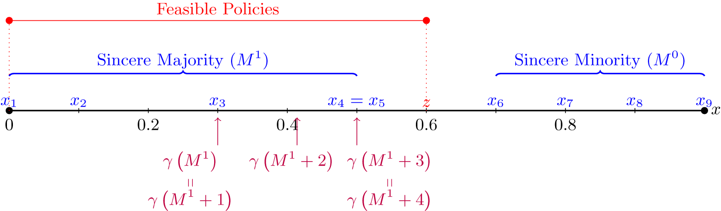
FIGURE 2. Equilibrium Policies for Differently Sized Dispositional Coalitions
TABLE 2. Equilibrium Coalitions that Implement Disposition d* = 1
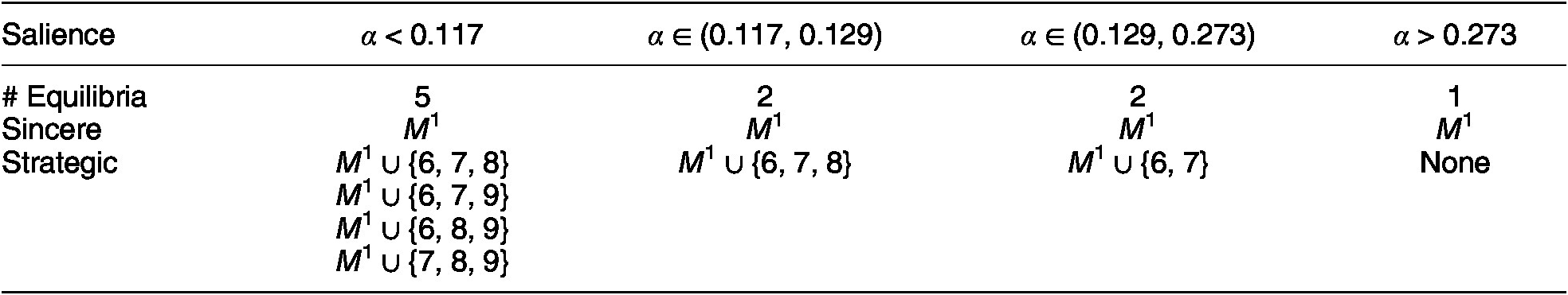
Note: Equilibria with sincere voting (i.e., the dispositional coalition is M 1) always exist. For α < 0.273, there are also equilibria in which judges in the sincere minority vote strategically. For α < 0.117, there can be multiple equilibria with strategic voting.
Unlike the policy subgame, where the equilibrium was unique, the strategic incentives at the adjudication stage result in there being potentially many adjudication (Nash) equilibria. There are two sources of multiplicity, both apparent in Example 4 and both having to do with coordination. For ease of exposition, suppose α < 0.117, so strategic voting is costly, but this cost is small relative to the resulting policy gains.
First, note that it is an equilibrium for any three of the four judges in the sincere minority to vote strategically. (There is no policy benefit to the fourth judge from voting strategically, and there is a policy cost to any of the three judges who voted strategically to switch to voting sincerely instead.) Because it does not matter which judges vote strategically and which one votes sincerely, there are four such equilibria. In this context, strategic voting by the judges exhibits “strategic substitutability.” The judges in the sincere minority are effectively playing a game of chicken—they face a coordination problem in deciding which judges will vote strategically and which will vote sincerely.
Second, it is also an equilibrium for all judges to vote sincerely. (There is no policy benefit to having one judge from the sincere minority vote strategically, as doing so does not shift the policy.) Therefore, strategic voting by the judges exhibits “strategic complementarity.” No judge would vote strategically if none of the others do. However, if at least one other judge voted strategically, then each of the remaining judges has an incentive to vote strategically as well. Starting from the sincere coalition, it takes a joint deviation by a group of judges to make strategic voting attractive.
The example also illustrates how the composition of dispositional coalitions responds to changes in the salience of expressive utility. As α increases, so does the cost of voting strategically, and so the possibility of sustaining various equilibria with strategic voting decreases. By the single-crossing property, the expressive cost of insincerity is higher for judges with more extreme ideal policies. Thus, as α increases, judge 9 is the first to cease voting strategically, then judge 8, and so on.
Given the presence of multiple equilibria, we seek to focus attention on the equilibrium that is most plausible. To identify this focal equilibrium, we use two refinement criteria, limiting attention to adjudication equilibria that are connected and coalition proof.
An adjudication equilibrium is connected if both the majority and minority dispositional coalitions are connected. If a coalition is disconnected, then it must be that a relatively moderate judge voted sincerely whereas a relatively extreme judge voted strategically. However, given the single-crossing property, strategic voting is more costly for relatively extreme judges than for moderate ones. Thus, it is more reasonable to expect moderate judges to vote strategically than extreme judges. It is also more “likely,” in the sense that strategic voting by the moderate judge can be sustained in equilibrium over a larger range of values of α than strategic voting by an extreme judge (as seen in Example 4). Thus, when there are multiple adjudication equilibria resulting from strategic substitutes, connectedness selects the one that is most plausible.
An adjudication equilibrium is coalition proof if (a) no individual judge would benefit from a unilateral deviation and (b) no stable group of judges could mutually benefit from a joint deviationFootnote 14 (see Bernheim, Peleg, and Whinston Reference Bernheim, Peleg and Whinston1987). The refinement rules out equilibria in which a subset of agents are trapped in a situation that is inferior but from which they could jointly and stably escape. On collegial courts, it is not unreasonable to assume that communication between the judges can enable a coalition of judges to jointly affect a favorable deviation. When strategic complementarity creates multiple equilibria, coalition proofness selects the equilibrium that is “most plausible,” in the sense of ensuring that those complementarities are exploited as far as possible. We show in Lemma 4 in the Appendix that the refinement selects the adjudication equilibrium with the “largest” coalition, guaranteeing that all complementarities are fully exhausted. A consequence is that equilibrium dispositional majorities exhibit greater (apparent) cohesion than would be the case if all judges voted sincerely.
We can apply the notions of connectedness and coalition-proofness to select a focal equilibrium from the multiplicity in Example 4 when α < 0.273. (When α > 0.273, there is a unique adjudication equilibrium, and so there is no selection to make.) First, note that when α < 0.117, connectedness rules out three of the four equilibria with strategic voting—the ones that require judge 9 to vote strategically. This is reasonable because judge 9 is most extreme and thus finds it most costly to vote strategically. Two candidate equilibria remain; the sincere equilibrium and the equilibrium in which judges 6, 7 (and for some values of α, judge 8) vote strategically. Coalition proofness selects the equilibrium with the larger majority coalition, consistent with strategic voting.
We are now ready to characterize the main results in this section.
Proposition 3. There exists a Connected Coalition-proof Adjudcation Equilibrium (CCPAE). Moreover, the following apply in any CCPAE (d, M):
-
• If d = 1, then M = {1,…, j 1}, where
$ {j}_1\hskip1.5pt \ge \hskip1.5pt \frac{n+1}{2} $
.
-
• If d = 0, then M = {j 0,…,n}, where
$ {j}_0\hskip1.5pt \le \hskip1.5pt \frac{n+1}{2} $
.


Proposition 3 shows that a CCPAE always exists—that is, there is (at least) one Nash equilibrium that survives the refinements that we impose. Proposition 3 also describes the features of equilibrium coalitions. In any CCPAE, the majority coalition will contain all but (possibly) the most extreme-right judges if the disposition is “1” or all but (possibly) the most extreme-left judges if the disposition is “0.” An immediate implication is that the median judge will always be in the dispositional majority, and so the median justice is pivotal over the case disposition. We stress that whereas the median justice is pivotal, the equilibrium disposition need not coincide with the median judge’s sincere assessment of the case; she may vote strategically (see Example 5).
A related implication of Proposition 3 is that the median judge will always be one of the decisive judges in the policy-making stage. However, unless the dispositional vote is unanimous, some other judge will also be decisive. To the extent that opinion writers have agenda-setting power, the median judge may still be able to implement her ideal policy if she is assigned to write the opinion. However, as this agenda-setting privilege disappears (i.e., as δ → 1), the median judge’s ideal policy will generically not be implemented. Instead, the equilibrium policy will be to either her left or right, depending on whether the majority coalition contains mostly leftist or rightist judges.
Whereas Proposition 3 guarantees that a CCPAE exists, it doesn’t guarantee that the CCPAE is unique.
Corollary 1. There exist at most two CCPAEs.
-
1. If (d, M) and (d′, M′) are distinct CCPAEs, then d ≠ d′.
-
2. For each z ∈ [0, 1], there exists α(z) ≥ 0 such that if α > α(z), the CCPAE is unique.
Corollary 1 tells us that there are no more than two CCPAEs. Part 1 tells us that if there are two CCPAEs, one will be associated with disposition d = 0 and the other with disposition d = 1. Thus, our refinements isolate the focal equilibrium associated with each of the two possible dispositional outcomes.
Part 2 tells us that as expressive preferences become sufficiently salient, there can only be one CCPAE. When the expressive cost of insincerity is large, sufficiently many judges will vote sincerely, and this will prevent one of the dispositional outcomes from arising in equilibrium. (In many scenarios, but not always, the prevailing outcome will be the one that would arise if all judges cast their dispositional votes sincerely.) By contrast, when α is low enough, policy preferences dominate the decision making of enough judges so that both outcomes can be sustained as equilibria. Judges are strongly motivated to be in the dispositional majority and thus affect policy making. The adjudication game resembles a dispositional coordination game. Most judges care less about which disposition prevails than about ensuring that they are part of the majority coalition. In particular, there will be equilibria in which a strong majority of judges favor one disposition, and yet the other disposition is chosen.
The following example illustrates each of the points discussed above:
Example 5.
Consider a case z = 0.55. Suppose that policy preferences are bell-curve shaped: $ {u}_P\left(y,x\right)={e}^{-\frac{1}{2}{\left(y-x\right)}^2}-1 $
, the disagreement payoff is uP
(D, x) = −1, and δ → 1. Let the ideal policies be x
1 = x
2 = x
3 = x
4 = 0 < x
5 = 0.5 < 0.7 = x
6 = x
7 = x
8 = x
9 (i.e., there is a relatively extreme homogeneous left bloc of four judges, a relatively moderate right bloc of four judges, and a centrist median judge). The median judge’s ideal disposition is d
* = 1.
Figure 3
illustrates this setup, and the equilibrium policies that will result, for each dispositional outcome, depending on whether the minority bloc votes strategically or not. The CCPAEs are described in
Table 3
.
$ {u}_P\left(y,x\right)={e}^{-\frac{1}{2}{\left(y-x\right)}^2}-1 $
, the disagreement payoff is uP
(D, x) = −1, and δ → 1. Let the ideal policies be x
1 = x
2 = x
3 = x
4 = 0 < x
5 = 0.5 < 0.7 = x
6 = x
7 = x
8 = x
9 (i.e., there is a relatively extreme homogeneous left bloc of four judges, a relatively moderate right bloc of four judges, and a centrist median judge). The median judge’s ideal disposition is d
* = 1.
Figure 3
illustrates this setup, and the equilibrium policies that will result, for each dispositional outcome, depending on whether the minority bloc votes strategically or not. The CCPAEs are described in
Table 3
.
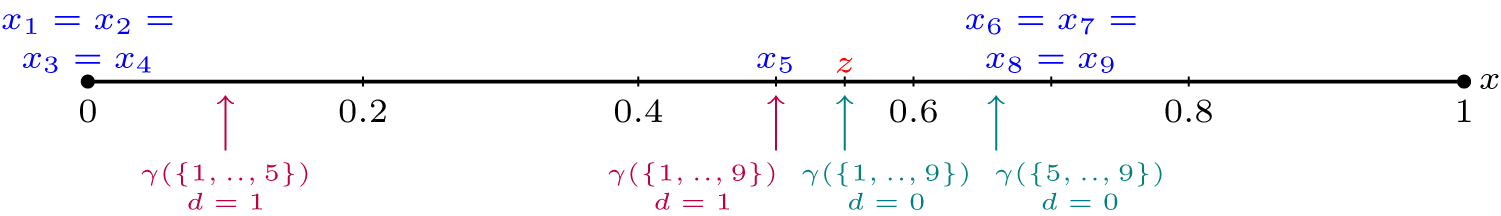
FIGURE 3. Equilibrium Policies Chosen for Differently Composed Dispositional Majorities
TABLE 3. CCPAE Equilibria in Example 5

There is a unique equilibrium whenever α > 0.5848 = α(z). Even when equilibria are unique (i.e., the median judge is pivotal), the outcome need not coincide with her ideal disposition. There will be strategic voting unless α > 1.2848. Moreover, as α increases, more extreme judges become less likely to vote strategically. Thus, the median judge potentially votes strategically over the largest range of α, whereas the left bloc of judges vote strategically over the smallest range. □
As Example 5 illustrates, when α is low, there is a CCPAE in which all judges, regardless of their actual preferences, choose disposition d = 1 and a CCPAE where they all choose disposition d = 0. A similar result arises in Fischman (Reference Fischman2011), although the mechanism is different. In Fischman’s model, unanimity arises because it is costly to dissent (for example, because it would require the judge to expend resources writing a dissenting opinion). In our model, unanimity arises because the hedonic cost of voting insincerely is low relative to the policy gains.
Comparative Statics
Effect of Salience of Expressive Utility
Example 5 showed that the incentives for judges to vote strategically varied with the salience of expressive preferences α, and the distance of the case from each judge’s ideal threshold. Intuitively, as expressive concerns become more salient, strategic voting becomes harder to sustain, and so the majority coalition shrinks in size. If expressive concerns are sufficiently large, then no judge will vote strategically, and equilibrium coalitions and case dispositions will reflect the sincere preferences of the judges.
Fix a case z. Let d(z) = 1[|M 1 (z)| > |M 0 (z)|] denote the sincere disposition, which is the disposition that would prevail if all judges voted sincerely. Similarly, let M(z) denote the sincere majority coalition: M(z) = M d(z)(z). The above ideas are reflected in Lemma 3 and are illustrated in Example 5 and Figure 4, below.
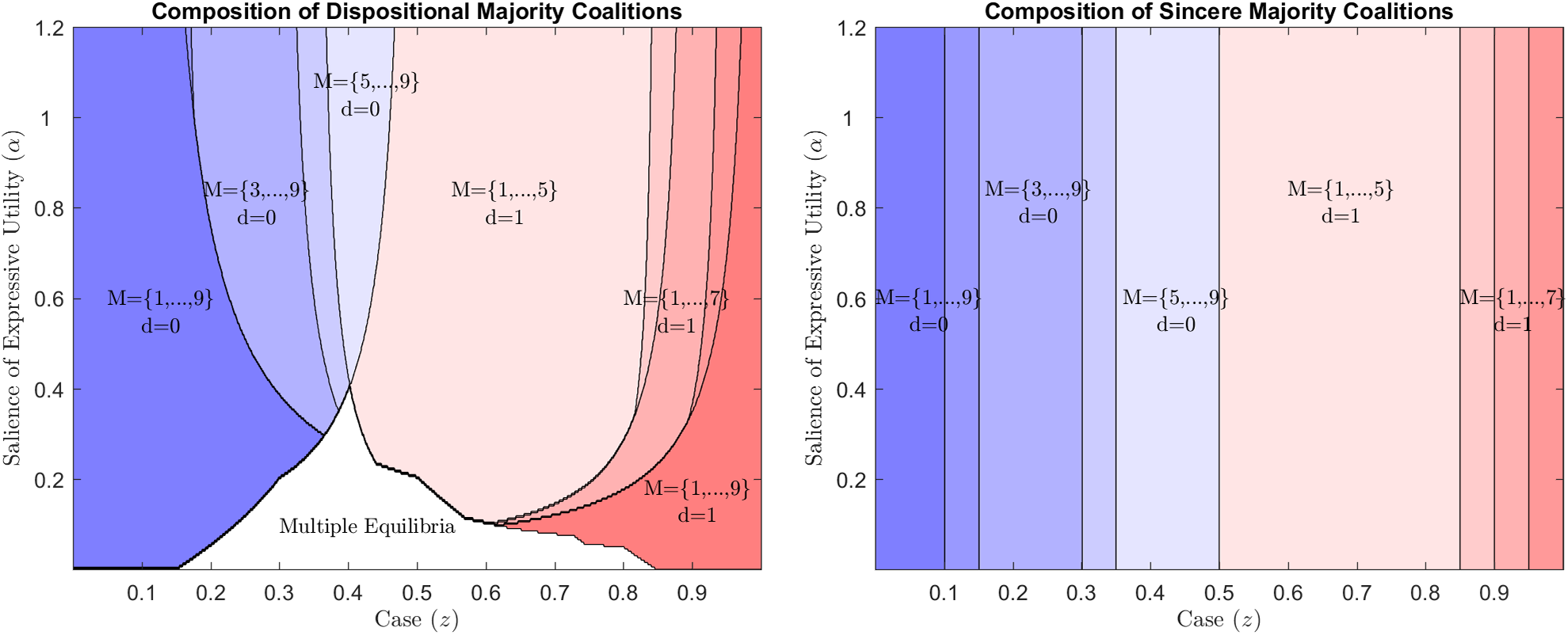
FIGURE 4. Effect of Case Location and the Salience of the Expressive Utility on the Composition of the Dispositional Majority, and the Resulting Policy
Note: Policy preferences are bell-curve shaped: $ {u}_P\left(y,x\right)={e}^{-\frac{1}{2}{\left(z-x\right)}^2}-1 $
, the disagreement payoff is uP
(D, x) = −1, and δ → 1. The vector of ideal policies is (x
1, …, x
9) = (0.1.0.15, 0.3, 0.35, 0.5, 0.85, 0.9, 0.95, 1). The left panel shows actual CCPAE dispositions and majority coalitions. The right panel shows dispositions and coalitions if the judges voted sincerely.
$ {u}_P\left(y,x\right)={e}^{-\frac{1}{2}{\left(z-x\right)}^2}-1 $
, the disagreement payoff is uP
(D, x) = −1, and δ → 1. The vector of ideal policies is (x
1, …, x
9) = (0.1.0.15, 0.3, 0.35, 0.5, 0.85, 0.9, 0.95, 1). The left panel shows actual CCPAE dispositions and majority coalitions. The right panel shows dispositions and coalitions if the judges voted sincerely.
Lemma 3. The following are true:
-
1. The size of equilibrium coalitions (with the same disposition) is decreasing in expressive concerns. Formally, let (d,M) and (d′,M′) be CCPAEs associated with salience levels α and α′, with α > α′. If d = d′, then M ⊆ M′.
-
2. When there are no expressive concerns, the Court’s decisions will be unanimous. (If α = 0, then M = {1,.., n}.)
-
3. When expressive concerns are sufficiently large, the unique CCPAE is characterized by sincere voting. (For a given case z, there exists
$ \overline{\alpha}(z)>0 $
s.t.
$ \forall \alpha >\overline{\alpha}(z) $
there is a unique CCPAE (d, M) with d = d(z) and M = M(z).)


Part 2 of the Lemma merits further comment. It states that the court will be unanimous in any CCPAE when expressive concerns are not salient.Footnote 15 In practice, on the Supreme Court, dissents by at least one judge are common, and 5–4 dispositional votes are not uncommon. Thus, we highlight the important role that expressive preferences play in describing behavior on the Court. Neither our model, nor any that is broadly similar, would be able to explain dissents if limited to judicial preferences that were purely consequentialist.Footnote 16
Effect of Case Location
A key insight of this paper is that rule-making by courts cannot be divorced from the specific facts of the case being adjudicated. (This stands in contrast to “legislature-like” models of the judiciary, where the court purely focuses on policy making, to which end the facts of the instant case are incidental.) Example 2 demonstrated that the case facts may directly affect the set of feasible policies that the Court could implement and that the dispositional consistency requirement might be binding.
Case location also affects the composition of the dispositional majority, and this will likely affect the equilibrium policy, even when the consistency constraint is nonbinding. This occurs for two reasons. First, suppose all judges cast dispositional votes sincerely. Then, starting from the median judge’s ideal threshold, as cases becomes more extreme, the number of judges who find themselves in the majority will (rather obviously) increase.
Second, and more subtly, changing the case location can change the incentives for judges to vote strategically and thus affect the composition of the dispositional majority. To see this, consider the example below, which considers two cases that would both result in the same dispositional majority if judges voted sincerely:
Example 6. Suppose that policy preferences and ideal policies are as in Example 5. Let α = 0.3. Consider two cases: z 1 = 0.1 and z 2 = 0.4. In both scenarios, the case is located between the ideal policy of the left bloc and the median judge so that the sincere disposition and sincere majority coalition would be d(zi ) = 0 and M(zi ) = {5,…, 9}. Both scenarios admit a unique CCPAE, with disposition d = 0.
-
• When z = 0.1, the majority coalition will be the entire bench M = {1,…, 9}, and the equilibrium policy will be γ = 0.5. There is strategic voting by the left bloc.
-
• When z = 0.4, the majority coalition will consist of a bare majority M = {5,…, 9} and the equilibrium policy will be γ = 0.66. There is no strategic voting.
In both scenarios, each judge would ideally decide the cases the same way. However, when z is close to the left bloc’s threshold, the cost of strategic voting is lower, and thus the judges are more inclined to vote strategically, to pull the ideal policy closer to their ideal. □
Although the set-up in Example 6 is stark, it reflects a more general relationship between case location, the composition of dispositional majorities, and the policy of the court. We see this general relationship in Figure 4 below:
The left panel of Figure 4 shows how the equilibrium dispositions and coalitions vary as a function of case location and the salience of expressive utility. The blue (towards the left) and red (towards the right) areas represent regions where the majority disposition is d = 0 and d = 1, respectively. Darker regions indicate larger coalitions. The right panel represents the disposition and majority coalitions if judges voted sincerely. These regions should be vertical bands, as the outcome under sincere voting is independent of α. Since the boundaries are vertical when judges vote sincerely, one way to observe the extent of strategic voting is to see how “sloped” or “curved” the boundaries of the regions are.
The results from Lemma 3 are also evident in Figure 4. First, fixing a case z, as α increases, the number of judges in the majority coalition decreases. The extent of strategic voting decreases as the salience of expressive utility increases. Second, as α becomes sufficiently large, the lines become vertical; for α large enough, the equilibrium coalitions coincide with the coalitions that would arise under sincere voting. Finally, fixing any α, we notice that as the case becomes more extreme, equilibrium coalitions are more likely to be larger and the likelihood of strategic voting increases. Indeed, since x 9 = 1, if judges voted sincerely, judge 9 would always choose d 9 = 0. However, allowing for strategic voting, judge 9 potentially chooses d = 1 over a large range of cases when α is low.
Tying the results from sections 3 and 4 together, then, yields the following insight. When the case is moderate (in the sense of being close to the median judge’s ideal threshold), then majority coalitions are likely to be smaller and the resulting equilibrium policy is likely to be more extreme (in the sense of being farther from the median judge’s ideal). As the case becomes more extreme (i.e., farther from the median judge’s threshold), then majority coalitions will become larger and the resulting policy will likely be more moderate (i.e., closer to the median judge’s ideal).
DISCUSSION
The model opens new avenues for studying institutions that jointly produce judgments and policies. To illustrate, we briefly discuss 9 empirical implications about decision making on the U.S. Supreme Court.
Strategic Dispositional Voting
Express indications of strategic voting are understandably rare among the justices. However, there are exceptions, such as Arizona v. Fulminante, which we noted in the Introduction. A small empirical literature examines strategic dispositional voting on the U.S. Supreme Court (Arrington and Brenner Reference Arrington and Brenner2004; Clark, Montagnes, and Spenkuch Reference Clark, Montagnes and Spenkuch2018; Johnson, Spriggs, and Wahlbeck Reference Johnson, Spriggs and Wahlbeck2005). In addition, studies of the Chief Justice often note his incentive to vote strategically on the disposition, to control the initial opinion assignment (cf. Maltzman and Wahlbeck Reference Maltzman and Wahlbeck1996). However, the absence of an explicit theory of strategic dispositional voting has limited these studies.Footnote 17 The sequential bargaining model points to a new approach by distinguishing likely sincere votes from possibly strategic ones. Contrasting the voting patterns for the same justice using the two types of votes becomes the critical comparison. More specifically,
-
1. The model predicts that dissents are always sincere, as are join versus concur decisions, whereas votes to join the dispositional majority may be strategic. Thus, the required test simply compares voting patterns by justice using votes sorted this way.
-
2. The model predicts that dispositional voting in high-α cases (those in which the disposition is critical but policy is not) is likely sincere, whereas voting in low-α cases (where dispositions matter little but policy is extremely important) may not be. Bush v. Gore, settling a recount dispute in Florida’s 2000 presidential election, illustrates a likely high-α case. The disposition of the case was clearly critical, as it determined the result of the election; the dispositional majority, moreover, sought to minimize the precedential value of the decision, stating, “Our consideration is limited to the present circumstances, for the problem of equal protection in election processes generally presents many complexities.”Footnote 18 This statement sought to render the policy unimportant. More systematically, many death penalty cases seem disposition-critical rather than policy-critical. Given the identification of sufficient number of high- and low-α cases, the required contrast in voting patterns by justice can be implemented.
-
3. The model predicts that strategic dispositional voting is less likely for justices located on the ideological wings of the Court than those located in the center of the Court. Some justices have served for extended periods during which they moved from wing to center or vice versa due to exogenous changes in the Court’s make-up. The resulting natural experiment offers an attractive venue for implementing the required contrast in decisions to join the dispositional majority.
Policy Coalitions
In the absence of theories explaining why policy coalitions matter, scholars have devoted little attention to them.Footnote 19 But because policy coalitions—defined by joins versus concurs in the dispositional majority—are easy to observe, they offer an attractive venue for testing models that actually make predictions about policy coalitions.Footnote 20 Our model offers the following testable predictions about policy coalitions.
-
4. Join coalitions will be connected, and built from one ideological side of the dispositional majority or the other but not from the center toward both wings. In other words, few join coalitions will feature “both ends against the middle” join/concur voting.
-
5. In cases where the bargaining intensity is very high (i.e., the parameter δ approaches 1) the size of the join coalition will approach 5.
-
6. By contrast, when bargaining intensity is very low (i.e., the parameter δ approaches 0), concurs will disappear. Thus, the join coalition will tend to include the entire dispositional majority.
Policy Content of Majority Opinions
The model makes many distinctive predictions about the policy content (spatial location) of majority opinions. Among the more striking are
-
7. Fixing the identity of the members of the majority dispositional coalition, there will be a distribution of majority opinion locations associated with the coalition, not a single location.
-
8. When bargaining intensity is high (i.e., δ approaches 1), the majority opinion locations will be drawn to the “center” of the dispositional majority, where that center is measured by the weighted Nash bargaining solution (a spatial location that can readily be calculated).
-
6. When bargaining intensity is low, (i.e, δ approaches 0) majority opinions will move closer to the ideal point of the opinion author; in other words, author influence will be greater.
These hypotheses await a solution to the tough measurement problem of locating majority opinions in the same space as justice ideal points. However, recent advances in scaling suggest that it may soon be feasible to test these (and other) hypotheses about majority opinion locations (see Clark and Lauderdale Reference Clark and Lauderdale2010).
CONCLUSION
In this paper, we present a new model of decision making on multimember bodies that simultaneously dispose of cases and formulate a rule that rationalizes the case disposition. We focus on one procedure, the “American procedure,” for joint production of judgments and policies. Although apex courts outside the United States use somewhat different procedures, scholars can adapt the analytic methods developed here to study those institutions as well.
We show that the American procedure leads to profound interactions between judgments and policies. As a result, treating the U.S. Supreme Court (for example) as a “little legislature” is problematic because it ignores how judgments tether policy outcomes. Similarly, treating the U.S. Supreme Court as a “big jury” may misrepresent judgments to a degree, because it ignores the possibility of strategic dispositional voting that is directed toward shaping subsequent policy making. The model makes specific predictions about dispositional coalitions, policy coalitions, and the content (spatial location) of majority opinions. These offer new directions for empirical studies.
There are obvious possibilities for further theoretical development. Case selection is a valuable one because case locations emerge as critical for both judgments and policy. Stare decisis and the time consistency of policy making is a second extension. For example, when will the Court obey its own precedents and when might it deviate from them? A valuable departure in comparative institutional analysis would extend the joint production framework to those used in non-American constitutional and international courts. Additionally, as with most formal models, our framework assumes that the judges’ preferences are common knowledge. In practice, some preference uncertainty may exist—although on Collegial courts, we think this concern will be more muted than in other settings—and this will naturally affect the equilibrium behavior of judges at both the policy and adjudication stage. We leave the analysis of behavior under asymmetric information of this sort to future studies.
Supplementary Materials
To view supplementary material for this article, please visit http://dx.doi.org/10.1017/S0003055421000083.
ACKNOWLEDGMENTS
The authors thank Scott Baker, Alvaro Bustos, John Duggan, Hulya Eraslan, Joshua Fischman, Barry Friedman, Sean Gailmard, Anna Harvey, Gleason Judd, Jeff Lax, Pablo Montagnes, Hunter Rendleman, Kathy Spier, Mike Ting, and seminar participants at Haverford College, University of West Virginia, the 2017 Law and Economic Theory Conference, the 2018 Princeton, Utah, and Warwick Conference on Political Economy, the 2018 American Law and Economics Association annual meeting, and the 2020 NBER Law and Economics Spring session.


 Open access