


1. Introduction
Long-dated contingent claims are relevant in insurance, pension fund management and derivative valuation. This paper proposes a shift in the valuation and production of long-term contracts, away from classical no-arbitrage valuation, towards less-expensive valuation under the real-world probability measure. In contrast to risk-neutral valuation, with the savings account as reference unit, the long-term best-performing portfolio, the numéraire portfolio of the equity market is coming into play in the proposed real-world valuation. A benchmark, the numéraire portfolio, is employed as the reference unit in the analysis, replacing the savings account. The numéraire portfolio is the strictly positive, tradable portfolio that when used as benchmark makes all benchmarked non-negative portfolios supermartingales. This means their current benchmarked values are greater than, or equal to, their expected future benchmarked values. Furthermore, the benchmarked real-world value of a benchmarked contingent claim is proposed to equal its real-world conditional expectation. This yields the minimal possible value for the benchmarked contingent claim. It turns out that the pooled total benchmarked hedge error of a well diversified book of contracts issued by an insurance company can practically vanish due to diversification when the number of contracts becomes large. In long-term asset and liability valuation, real-world valuation can lead to significantly lower values than suggested by classical valuation arguments where the existence of some equivalent risk-neutral probability measure is assumed.
Under the benchmark approach (BA), described in Platen & Heath (Reference Platen and Heath2010), instead of relying on the domestic savings account as the reference unit, a benchmark in form of the best performing, tradable strictly positive portfolio is chosen as numéraire. More precisely, it employs the numéraire portfolio as benchmark, whose origin can be traced back to Long (Reference Long1990), and which is equal to the growth optimal portfolio; see Kelly (Reference Kelly1956). In Bühlmann & Platen (Reference Bühlmann and Platen2003), a discrete time version of the BA was introduced into the actuarial literature. The current paper aims to popularise its continuous time version, which allows one to produce long-term payoffs less expensively than the classical risk-neutral production methodology.
In recent years, the problem of accurately valuing long-term assets and liabilities, held by insurance companies, banks and pension funds, has become increasingly important. How these institutions perform such valuations often remains unclear. The recent experience with low interest rate environments and the economic impacts of a pandemic suggests that some major changes are due in these industries concerning the valuation and production methods employed. One possible explanation for the need of change, to be explored in this article, is that the risk-neutral valuation paradigm itself may be too expensive, especially when it is applied to the valuation of long-term contracts. It leads to a more expensive production method than necessary, as will be explained in the current paper.
The structure of the paper is as follows: section 2 gives a brief survey on the literature about valuation methods in insurance and finance. Section 3 introduces the benchmark approach (BA). Real-world valuation is described in section 4. Three examples on real-world valuation and hedging of long-term annuities, with annual payments linked to a mortality index, a savings account or an equity index, possibly involving a guaranteed death benefit equal to a roll-up of initial premium, are illustrated in section 5. Section 6 concludes.
2. Valuation methods for long-term contracts
One of the most dynamic areas in the current risk management literature is the valuation of long-term contracts, including variable annuities. The latter represent long-term contracts with payoffs that depend on insured events and on underlying assets that are traded in financial markets. The valuation methods can be categorised into three main types: actuarial valuation or expected present value, risk-neutral valuation and utility maximisation valuation.
Actuarial valuation (expected present value)
One of the pioneers of calculating present values of contingent claims for life insurance companies was James Dodson, whose work is described in the historical accounts of Turnbull (Reference Turnbull2016) and Dodson (Reference Dodson1995). The application of such methods to with-profits policies ensued. In the late 1960s, US life insurers entered the variable annuity market, as mentioned in Sloane (Reference Sloane1970), where such products required assumptions on the long-term behaviour of equity markets. Many authors have analysed various actuarial models of the long-term evolution of stochastic equity markets, such as Wise (Reference Wise1984b) and Wilkie (Reference Wilkie1985, Reference Wilkie1987, Reference Wilkie1995).
Since the work of Redington (Reference Redington1952), the matching of well-defined cash flows with liquidly traded ones, while minimising the risk of reserves, has been a widely used valuation method in insurance. For instance, Wise (Reference Wise1984a,b, Reference Wise1987a, b, Reference Wise1989), Wilkie (Reference Wilkie1985) and Keel & Müller (Reference Keel and Müller1995) study contracts when a perfect match is not possible.
Risk-neutral naluation
The main stream of research, however, follows the concept of no-arbitrage valuation in the sense of Ross (Reference Ross1976) and Harrison & Kreps (Reference Harrison and Kreps1979). This approach has been widely used in finance, where it appears in the guise of risk-neutral valuation. The earliest applications of no-arbitrage valuation to variable annuities are in the papers by Brennan & Schwartz (Reference Brennan and Schwartz1976, Reference Brennan and Schwartz1979) and Boyle & Schwartz (Reference Boyle and Schwartz1977), which extend the Black-Scholes-Merton option valuation (see Black & Scholes Reference Black and Scholes1973 and Merton Reference Merton1973) to the case of equity-linked insurance contracts.
The Fundamental Theorem of Asset Pricing, in its most general form formulated by Delbaen & Schachermayer (Reference Delbaen and Schachermayer1998), establishes a correspondence between the “no free lunch with vanishing risk” no-arbitrage concept and the existence of an equivalent risk-neutral probability measure. This important result demonstrates that theoretically founded classical no-arbitrage pricing requires the restrictive assumption that an equivalent risk-neutral probability measure must exist. In such a setting, the effect of stochastic interest rates on the risk-neutral value of a guarantee is crucial in insurance and has been discussed by many authors, such as Bacinello & Ortu (Reference Bacinello and Ortu1993, Reference Bacinello and Ortu1996), Aase & Persson (Reference Aase and Persson1994) and Huang & Cairns (Reference Huang and Cairns2004, Reference Huang and Cairns2005).
Risk-neutral valuation for incomplete markets
In reality, one has to deal with the fact that markets are incomplete and insurance payments are not fully hedgeable. The choice of a risk-neutral pricing measure is, therefore, not unique, as pointed out by Föllmer & Sondermann (Reference Föllmer and Sondermann1986) and Föllmer & Schweizer (Reference Föllmer and Schweizer1991), for example. Hofmann et al. (Reference Hofmann, Platen and Schweizer1992), Gerber & Shiu (Reference Gerber and Shiu1994), Gerber (Reference Gerber1997). Jaimungal & Young (Reference Jaimungal and Young2005), Duffie & Richardson (Reference Duffie and Richardson1991) and Schweizer (Reference Schweizer1992) address this issue by suggesting certain mean-variance hedging methods based on a form of variance- or risk-minimising objective, assuming the existence of a particular risk-neutral measure. In the latter case, the so-called minimal equivalent martingale measure, due to Föllmer & Schweizer (Reference Föllmer and Schweizer1991), emerges as the pricing measure. This valuation method is also known as local risk minimisation and was considered by Möller (Reference Möller1998, Reference Möller2001), Schweizer (Reference Schweizer2001) and Dahl & Möller (Reference Dahl and Möller2006) for the valuation of insurance products.
Expected utility maximisation
Another approach involves the maximisation of expected terminal utility, see Karatzas et al. (Reference Karatzas, Shreve, Lehoczky and Xu1991), Kramkov & Schachermayer (Reference Kramkov and Schachermayer1999) and Delbaen et al. (Reference Delbaen, Grandits, Rheinländer, Samperi, Schweizer and Stricker2002). In this case, the valuation is based on a particular form of utility indifference pricing. This form of valuation has been applied by Hodges & Neuberger (Reference Hodges and Neuberger1989) and later by Davis (Reference Davis1997) and others. It has been used to value equity-linked insurance products by Young & Zariphopoulou (Reference Young and Zariphopoulou2002a, b), Young (Reference Young2003) and Moore & Young (Reference Moore and Young2003).
Typically in the context of some expected utility maximisation, there is an ongoing debate on the links between the valuation of insurance liabilities and financial economics for which the reader can be referred to Reitano (Reference Reitano1997), Longley-Cook (Reference Longley-Cook1998), Babbel & Merrill (Reference Babbel and Merrill1998), Möller (Reference Möller1998, Reference Möller2002), Phillips et al. (Reference Phillips, Cummins and Allen1998), Girard (Reference Girard2000), Lane (Reference Lane2000) and Wang (Reference Wang2000, Reference Wang2002). Equilibrium modelling from a macro-economic perspective has been the focus of a line of research that can be traced back to Debreu (Reference Debreu1982), Starr (Reference Starr1997) and Duffie (Reference Duffie2001).
Stochastic discount factors
Several no-arbitrage pricing concepts have been popular in finance that are equivalent to the risk-neutral approach. For instance, Cochrane (Reference Cochrane2001) employs the notion of a stochastic discount factor. The use of a state-price density, a deflator or a pricing kernel has been considered by Constantinides (Reference Constantinides1992), Cochrane (Reference Cochrane2001) and Duffie (Reference Duffie2001), respectively. Another way of describing classical no-arbitrage pricing was pioneered by Long (Reference Long1990) and further developed in Bajeux-Besnainou & Portait (Reference Bajeux-Besnainou and Portait1997) and Becherer (Reference Becherer2001), who use the numéraire portfolio as numéraire instead of the savings account and employ the real-world probability measure as pricing measure to recover risk-neutral prices.
Real-world valuation under the benchmark approach
The previously mentioned line of research involving the numéraire portfolio comes closest to the form of real-world valuation under the benchmark approach (BA) proposed in Platen (Reference Platen2002b) and Platen & Heath (Reference Platen and Heath2010). The primary difference is that the BA no longer assumes the existence of an equivalent risk-neutral probability measure. In so doing, it allows for a much richer class of models to be available for consideration and permits several self-financing portfolios to replicate the same contingent claim, where it can select the least expensive one as corresponding production process. Even in a complete market, the BA can hedge less expensively many typical payoffs than classical no-arbitrage pricing allows. Throughout this article, we use the terms replicate and hedge interchangeably in respect of the payoff of a given contingent claim.
The BA employs the best-performing, strictly positive, tradable portfolio as benchmark and makes it the central reference unit for modelling, valuation and hedging. A well-diversified equity index can be used as benchmark, as explained in Platen & Heath (Reference Platen and Heath2010) and Platen & Rendek (Reference Platen and Rendek2012). In some sense, real-world valuation can be interpreted along the lines of budgeting. Since we will demonstrate that one can hedge real-world values, it is about calculating what a contingent claim is expected to cost when producing it through hedging.
All valuations are performed under the real-world probability measure and, therefore, labelled “real-world valuations.” When an equivalent risk-neutral probability measure exists for a complete market model, real-world valuation yields the same value as risk-neutral valuation. When there is no equivalent risk-neutral probability measure for the market model, then risk-neutral prices can still be employed, as we demonstrate in the paper, but these are usually more expensive than the respective real-world prices.
In Du & Platen (Reference Du and Platen2016), the concept of benchmarked risk minimisation has been introduced, which yields via the real-world value the minimal possible value of a not fully hedgeable contingent claim and minimizes the fluctuations of the profit and losses when denominated in units of the numéraire portfolio. The profit and loss for the hedge portfolio of a contingent claim is defined as the theoretical value minus the realized gains from trade minus the initial value. Risk minimisation that is close to the previously mentioned concept of local risk minimisation of Föllmer & Schweizer (Reference Föllmer and Schweizer1991) and Föllmer & Sondermann (Reference Föllmer and Sondermann1986) was studied under the benchmark approach in Biagini et al. (Reference Biagini, Cretarola and Platen2014).
Stochastic mortality rates
Note that stochastic mortality rates are easily incorporated in the pricing of insurance products as demonstrated by Milevsky & Promislow (Reference Milevsky and Promislow2001), Dahl (Reference Dahl2004), Kirch & Melnikov (Reference Kirch and Melnikov2005), Cairns et al. (Reference Cairns, Blake and Dowd2006a, b, 2008), Biffis (Reference Biffis2005), Melnikov & Romaniuk (Reference Melnikov and Romaniuk2006, Reference Melnikov and Romaniuk2008) and Jalen & Mamon (Reference Jalen and Mamon2008). Most of these authors assume that the market is complete with respect to mortality risk, which means that it can be removed by diversification.
3. Benchmark approach
Since it will be crucial for the less-expensive production method, we propose in this paper, and since the continuous time BA has not been outlined in an actuarial journal, we will give within this and the following sections a survey about the BA, which goes beyond results presented in Platen (Reference Platen2002b) and Platen & Heath (Reference Platen and Heath2010). Consider a market comprising a finite number $J+1$
of primary security accounts. An example of such a security could be an account containing shares of a company with all dividends reinvested in that stock. A savings account held in some currency is another example of a primary security account. In reality, time is continuous, and this paper considers continuous time models that are described by Itô stochastic differential equations. These can provide compact and elegant mathematical descriptions of asset value dynamics. We work on a filtered probability space
$J+1$
of primary security accounts. An example of such a security could be an account containing shares of a company with all dividends reinvested in that stock. A savings account held in some currency is another example of a primary security account. In reality, time is continuous, and this paper considers continuous time models that are described by Itô stochastic differential equations. These can provide compact and elegant mathematical descriptions of asset value dynamics. We work on a filtered probability space $(\Omega , {\mathcal{F}},{\underline{\mathcal{F}}} , P )$
with filtration
$(\Omega , {\mathcal{F}},{\underline{\mathcal{F}}} , P )$
with filtration ${\underline{\mathcal{F}}} = ({\mathcal{F}}_t)_{t\ge 0}$
satisfying the usual conditions, as in Karatzas & Shreve (Reference Karatzas and Shreve1991).
${\underline{\mathcal{F}}} = ({\mathcal{F}}_t)_{t\ge 0}$
satisfying the usual conditions, as in Karatzas & Shreve (Reference Karatzas and Shreve1991).
The key assumption of the BA is that there exists a best-performing, strictly positive, tradable portfolio in the given investment universe, which we specify later on as the numéraire portfolio. This benchmark portfolio can be interpreted as a universal currency. Its existence turns out to be sufficient for the formulation of powerful results concerning diversification, portfolio optimisation and valuation.
The benchmarked value of a security represents its value denominated in units of the benchmark, the numéraire portfolio. Denote by ${\hat{S}}^j_t$
the benchmarked value of the jth primary security account,
${\hat{S}}^j_t$
the benchmarked value of the jth primary security account, $j \in \{ 0,1,\ldots ,J\}$
, at time
$j \in \{ 0,1,\ldots ,J\}$
, at time $t \geq 0$
. The 0-th primary security account is chosen to be the savings account of the domestic currency. The particular dynamics of the primary security accounts are not important for the formulation of several statements presented below. For simplicity, taxes and transaction costs are neglected in the paper.
$t \geq 0$
. The 0-th primary security account is chosen to be the savings account of the domestic currency. The particular dynamics of the primary security accounts are not important for the formulation of several statements presented below. For simplicity, taxes and transaction costs are neglected in the paper.
The market participants can form self-financing portfolios with primary security accounts as constituents. A portfolio at time t is characterized by the number $\delta^j_t$
of units held in the jth primary security account,
$\delta^j_t$
of units held in the jth primary security account, $j \in \{ 0,1,2,\ldots ,J \}$
,
$j \in \{ 0,1,2,\ldots ,J \}$
, $t \geq 0$
. Assume for any given strategy
$t \geq 0$
. Assume for any given strategy $\delta=\{\delta_t=(\delta^0_t,\delta^1_t,\ldots , \delta^J_t )^\top, t \geq 0 \}$
that the values
$\delta=\{\delta_t=(\delta^0_t,\delta^1_t,\ldots , \delta^J_t )^\top, t \geq 0 \}$
that the values $\delta^0_t,\delta^1_t,\ldots ,\delta^J_t $
depend only on information available at the time t. The value of the benchmarked portfolio, which means its value denominated in units of the benchmark, is given at time t by the sum
$\delta^0_t,\delta^1_t,\ldots ,\delta^J_t $
depend only on information available at the time t. The value of the benchmarked portfolio, which means its value denominated in units of the benchmark, is given at time t by the sum
 \begin{equation} {\hat{S}}^\delta_t = \sum_{j=0}^J \delta^j_t\,{\hat{S}}^j_t, \end{equation}
for $t \geq 0$
. Since at any finite time, there is only finite total wealth available in the market, the paper considers only strategies whose benchmark and associated benchmarked portfolio values remain finite at all finite times.
$t \geq 0$
. Since at any finite time, there is only finite total wealth available in the market, the paper considers only strategies whose benchmark and associated benchmarked portfolio values remain finite at all finite times.
Let $E_t(X)=E(X|{\mathcal{F}}_t)$
denote the expectation of a random variable X under the real-world probability measure P, conditioned on the information available at time t captured by
$E_t(X)=E(X|{\mathcal{F}}_t)$
denote the expectation of a random variable X under the real-world probability measure P, conditioned on the information available at time t captured by ${\mathcal{F}}_t$
(e.g. see section 8 of Chapter 1 of Shiryaev Reference Shiryaev1984). This allows us to formulate the main assumption of the BA as follows:
${\mathcal{F}}_t$
(e.g. see section 8 of Chapter 1 of Shiryaev Reference Shiryaev1984). This allows us to formulate the main assumption of the BA as follows:
Assumption 1. There exists a strictly positive benchmark, called the numéraire portfolio (NP), such that each benchmarked non-negative portfolio ${\hat{S}}^\delta_t$
forms a supermartingale, which means that
${\hat{S}}^\delta_t$
forms a supermartingale, which means that
 \begin{equation} {\hat{S}}^\delta_t \geq E_t({\hat{S}}^\delta_s) \end{equation}
for all $0 \leq t \leq s < \infty$
.
$0 \leq t \leq s < \infty$
.
Inequality (2) can be referred to as the supermartingale property of benchmarked securities. It is obvious that the benchmark represents in the sense of (2) the best-performing portfolio, forcing all benchmarked non-negative portfolios in the mean downward or having no trend. In general, the numéraire portfolio (NP) coincides with the growth optimal portfolio, which is the portfolio that maximizes expected logarithmic utility, see Kelly (Reference Kelly1956). Since only the existence of the numéraire portfolio is requested, the benchmark approach reaches beyond the classical no-arbitrage modelling world.
According to Assumption 1, the current benchmarked value of a non-negative portfolio is greater than or equal to its expected future benchmarked values. Assumption 1 guarantees several fundamental properties of any useful financial market model without assuming a particular dynamic for the asset values. For example, it implies the absence of economically meaningful arbitrage, which means that any strictly positive portfolio remains finite at any finite time because the best-performing portfolio, the NP, has this property. As a consequence of the supermartingale property (2) and because a non-negative supermartingale that reaches zero is absorbed at zero, no wealth can be created from zero initial capital under limited liability.
Recall that for the classical risk-neutral valuation, the corresponding no-arbitrage concept is formalised as “no free lunch with vanishing risk” (NFLVR); see Delbaen & Schachermayer (Reference Delbaen and Schachermayer1994). The BA assumes that the portfolio remains finite at any finite time, which is equivalent to the “no unbounded profits with bounded risk” (NUPBR) no-arbitrage concept, see Karatzas & Kardaras (Reference Karatzas and Kardaras2007). Under the BA, an equivalent martingale measure is not required to exist, and therefore, benchmarked portfolio strategies are permitted to form strict supermartingales and not only martigales, a phenomenon which we exploit in the current paper.
Another fundamental property that follows directly from the supermartingale property (2) is that the benchmark, the NP, is unique. To see this, consider two strictly positive portfolios that are supposed to represent the benchmark. The first portfolio, when expressed in units of the second one, must satisfy the supermartingale property (2). By the same argument, the second portfolio, when expressed in units of the first one, must also satisfy the supermartingale property. Consequently, by Jensen’s inequality both portfolios must be identical. Thus, the value process of the benchmark that starts with given strictly positive initial capital is unique. Due to possible redundancies in the set of primary security accounts, this does not imply uniqueness for the trading strategy generating the benchmark.
Assumption 1 is satisfied for any reasonable financial market model. It simply asserts the existence of a best performing portfolio that does not reach infinity at any finite time. This requirement can be interpreted as the absence of economically meaningful arbitrage, which means that the benchmark and all associated benchmarked self-financing portfolios remain finite at finite times. In Theorem 14.1.7 of Chapter 14 of Platen & Heath (Reference Platen and Heath2010), Assumption 1 has been verified for jump diffusion markets, which cover a wide range of possible market dynamics. Karatzas & Kardaras (Reference Karatzas and Kardaras2007) and Christensen & Larsen (Reference Christensen and Larsen2007) show that Assumption 1 is satisfied for any reasonable semimartingale model. Note that Assumption 1 permits us to model benchmarked primary security accounts that are not martingales. This is necessary for realistic long-term market modelling, as will be demonstrated in section 5.
By referring to results in Platen (Reference Platen2004), Le & Platen (Reference Le and Platen2006), Platen & Rendek (Reference Platen and Rendek2012) and (2017), one can say that the benchmark portfolio is not only a theoretical construct, but can be approximated by well diversified portfolios, for example by the MSCI world stock index for the global equity market or the S $\&$
P500 total return index for the US equity market.
$\&$
P500 total return index for the US equity market.
A special type of security emerges when equality holds in relation (2).
Definition. A security is called fair if its benchmarked value ${\hat{V}}_t$
forms a martingale; that is, the current value of the process
${\hat{V}}_t$
forms a martingale; that is, the current value of the process $\hat{V}$
is the best forecast of its future values, which means that
$\hat{V}$
is the best forecast of its future values, which means that
 \begin{equation} {\hat{V}}_t = E_t\left( {\hat{V}}_s\right) \end{equation}
for all $0 \leq t \leq s < \infty$
.
$0 \leq t \leq s < \infty$
.
Note that the above notion of a fair security is employing the NP, the benchmark. The BA allows us to consider securities that are not fair. This important flexibility is missing in the classical no-arbitrage approach, which essentially assumes always equality in (3). Securities that are not fair will be required when modelling the market realistically over long time periods.
4. Real-world valuation
As stated earlier, the most obvious difference between the BA and the classical risk-neutral approach is the choice of the pricing measure. The former uses the real-world probability measure with the NP as numéraire for valuation, while the savings account is the chosen numéraire under the risk-neutral approach, which assumes the existence of an equivalent risk-neutral probability measure. Under the risk-neutral approach, this assumption is additionally imposed to our Assumption 1 and, therefore, reduces significantly the class of models and phenomena considered. The supermartingale property (2) ensures that the expected return of a benchmarked non-negative portfolio can be at most zero. In the case of a fair benchmarked portfolio, the expected return is precisely zero. The current benchmarked value of such a portfolio is, therefore, the best forecast of its benchmarked future values. The risk-neutral approach assumes that for complete markets the savings account is fair, which seems to be at odds with evidence; see for example Baldeaux et al. (Reference Baldeaux, Grasselli and Platen2015) and (Reference Baldeaux, Ignatieva and Platen2018).
Under the benchmark approach, there can be many supermartingales that approach the same future random value of a payoff. In other words, there are many portfolio strategies which replicate the same given contingent claim $H_T$
at a future time T. Among such portfolio strategies, we identify the minimal replicating portfolio strategy to determine the portfolio which replicates the payoff
$H_T$
at a future time T. Among such portfolio strategies, we identify the minimal replicating portfolio strategy to determine the portfolio which replicates the payoff $H_T$
with the smallest initial value. Within a family of non-negative supermartingales, the supermartingale with the smallest initial value turns out to be the corresponding martingale; see Proposition 3.3 in Du & Platen (Reference Du and Platen2016). This basic fact allows us to deduce directly the following Law of the Minimal Price:
$H_T$
with the smallest initial value. Within a family of non-negative supermartingales, the supermartingale with the smallest initial value turns out to be the corresponding martingale; see Proposition 3.3 in Du & Platen (Reference Du and Platen2016). This basic fact allows us to deduce directly the following Law of the Minimal Price:
Theorem. (Law of the Minimal Price) If a fair portfolio replicates a given non-negative payoff at some future time, then this portfolio represents the minimal replicating portfolio among all non-negative portfolios that replicate this payoff.
For a given payoff, there may exist self-financing replicating portfolios that are not fair. Consequently, the classical Law of One Price is no longer enforced under the BA. However, the above Law of the Minimal Price provides instead a consistent, unique minimal value system for all hedgeable contracts with finite expected benchmarked payoffs. When contingent claims are priced by formally applying the risk-neutral pricing rule, which currently seems widely practised, no economically meaningful arbitrage can be made from holdings in the savings account, the contingent claim and the underlying asset. However, such prices are not always minimal and, therefore, can be more expensive than necessary.
It follows for a given hedgeable payoff that the corresponding fair hedge portfolio represents the least expensive hedge portfolio. From an economic point of view, investors prefer more to less and this is, therefore, also the value in a liquid, competitive market where diversifiable uncertainty is diversified. As will be demonstrated in section 5, there may exist several self-financing portfolios that hedge one and the same payoff. It is the fair portfolio that hedges the payoff at minimal cost. We emphasize that risk-neutral valuation, based purely on hedging via classical no-arbitrage arguments, see Ross (Reference Ross1976) and Harrison & Kreps (Reference Harrison and Kreps1979), may lead to more expensive values than those given by the corresponding fair value.
Now, consider the problem of valuing a given payoff to be delivered at a maturity date $T \in (0,\infty)$
. Define a benchmarked contingent claim
$T \in (0,\infty)$
. Define a benchmarked contingent claim ${\hat{H}}_T$
as a non-negative,
${\hat{H}}_T$
as a non-negative, $\mathcal{F}_T$
measurable payoff denominated in units of the benchmark with finite expectation
$\mathcal{F}_T$
measurable payoff denominated in units of the benchmark with finite expectation
 \begin{equation} E_0 \left( {\hat{H}}_T\right) < \infty. \end{equation}
If for a benchmarked contingent claim ${\hat{H}}_T$
,
${\hat{H}}_T$
, $T \in(0, \infty)$
, there exists a benchmarked fair portfolio
$T \in(0, \infty)$
, there exists a benchmarked fair portfolio ${\hat{S}}^{\delta_{\hat{H}_T}}$
, which replicates this claim at maturity T, that is
${\hat{S}}^{\delta_{\hat{H}_T}}$
, which replicates this claim at maturity T, that is ${\hat{H}}_T ={\hat{S}}^{\delta_{\hat{H}_T}}_T$
, then, by the above Law of the Minimal Price, its minimal replicating benchmarked value process is at time
${\hat{H}}_T ={\hat{S}}^{\delta_{\hat{H}_T}}_T$
, then, by the above Law of the Minimal Price, its minimal replicating benchmarked value process is at time $t \in[0,T]$
given by the real-world conditional expectation
$t \in[0,T]$
given by the real-world conditional expectation
 \begin{equation} {\hat{S}}^{\delta_{\hat{H}_T}}_t = E_t \left( {\hat{H}}_T \right). \end{equation}
Multiplying both sides of equation (5) by the value of the benchmark in domestic currency at time t, denoted by $S^*_t$
, one obtains the real-world valuation formula
$S^*_t$
, one obtains the real-world valuation formula
 \begin{equation} S^{\delta_{\hat{H}_T}}_t = \hat{S}^{\delta_{\hat{H}_T}}_t \, S^*_t = S^*_t\, E_t \left( \frac{H_T}{S^*_T} \right) , \end{equation}
where $H_T={\hat{H}}_T\,S^*_T$
is the payoff denominated in domestic currency and
$H_T={\hat{H}}_T\,S^*_T$
is the payoff denominated in domestic currency and $S^{\delta_{\hat{H}_T}}_t$
the fair value at time
$S^{\delta_{\hat{H}_T}}_t$
the fair value at time $t \in [0,T]$
denominated in domestic currency.
$t \in [0,T]$
denominated in domestic currency.
Formula (6) is called the real-world valuation formula because it involves the conditional expectation $E_t$
with respect to the real-world probability measure P. It only requires the existence of the numéraire portfolio and the finiteness of the expectation in (4). These two conditions can hardly be weakened. By introducing the concept of benchmarked risk minimisation in Du & Platen (Reference Du and Platen2016), it has been shown that the above real-world valuation formula also provides the natural valuation for non-hedgeable contingent claims when one aims to diversify as much as possible the benchmarked non-hedgeable parts of contingent claims.
$E_t$
with respect to the real-world probability measure P. It only requires the existence of the numéraire portfolio and the finiteness of the expectation in (4). These two conditions can hardly be weakened. By introducing the concept of benchmarked risk minimisation in Du & Platen (Reference Du and Platen2016), it has been shown that the above real-world valuation formula also provides the natural valuation for non-hedgeable contingent claims when one aims to diversify as much as possible the benchmarked non-hedgeable parts of contingent claims.
An important application for the real-world valuation formula (6) arises when $H_T$
is independent of
$H_T$
is independent of $S^*_T$
, which leads to the generalized actuarial valuation formula
$S^*_T$
, which leads to the generalized actuarial valuation formula
 \begin{equation} S^{\delta_{{\hat{H}}_T}}_t =P(t,T)\,E_t(H_T). \end{equation}
The derivation of (7) from (6) exploits the fact that the expectation of a product of independent random variables equals the product of their expectations. One discounts in (7) by multiplying the real-world expectation $E_t(H_T)$
with the fair zero coupon bond value
$E_t(H_T)$
with the fair zero coupon bond value
 \begin{equation} P(t,T) = S^*_t\,E_t\left( (S^*_T)^{-1}\right). \end{equation}
Note that the fair zero coupon bond is under realistic assumptions less expensive than the respective classical risk-neutral zero coupon bond. When using the risk-neutral zero coupon bond in (7), then the actuarial valuation formula emerges, which has been used as a valuation rule by actuaries for centuries to determine the net present value of a claim. This important formula follows here under respective assumptions as a direct consequence of real-world valuation.
The following discussion aims to highlight the link between real-world valuation and risk-neutral valuation. Risk-neutral valuation uses as its numéraire the domestic savings account process $S^0=\{S^0_t \, , \, t \geq 0 \}$
, denominated in units of the domestic currency. Under certain assumptions, which will be described below, one obtains risk-neutral values from the real-world valuation formula by rewriting the real-world valuation formula (6) in the form
$S^0=\{S^0_t \, , \, t \geq 0 \}$
, denominated in units of the domestic currency. Under certain assumptions, which will be described below, one obtains risk-neutral values from the real-world valuation formula by rewriting the real-world valuation formula (6) in the form
 \begin{equation} S^{\delta_{{\hat{H}}_T}}_t = E_t \left( \frac{\Lambda_T}{\Lambda_t} \,\frac{S^0_t}{S^0_T} \,H_T \right) , \end{equation}
employing the normalized benchmarked savings account $\Lambda_t = \frac{S^0_t\,S^*_0}{S^*_t\,S^0_0}$
for
$\Lambda_t = \frac{S^0_t\,S^*_0}{S^*_t\,S^0_0}$
for $t \in [0,T]$
. Note that
$t \in [0,T]$
. Note that $\Lambda_0=1$
and when assuming that the putative risk-neutral measure Q is an equivalent probability measure we get
$\Lambda_0=1$
and when assuming that the putative risk-neutral measure Q is an equivalent probability measure we get
 \begin{equation} E_t \left( \frac{\Lambda_T}{\Lambda_t} \,\frac{S^0_t}{S^0_T} \,H_T \right) = E_t^Q \left( \frac{S^0_t}{S^0_T} \,H_T \right) , \end{equation}
because $\Lambda_t$
represents the respective (Radon-Nikodym derivative) density for Q at time t and
$\Lambda_t$
represents the respective (Radon-Nikodym derivative) density for Q at time t and $E^Q_t$
denotes the conditional expectation under Q. We remark that Q is an equivalent probability measure if and only if
$E^Q_t$
denotes the conditional expectation under Q. We remark that Q is an equivalent probability measure if and only if $\Lambda_t$
forms a true martingale, which means that the benchmarked savings account
$\Lambda_t$
forms a true martingale, which means that the benchmarked savings account ${\hat{S}}^0_t$
needs to form in this case a true martingale. It is the assumption of this restrictive martingale property that appears to be unrealistic for long-term modelling and leads to the current unnecessarily expensive production costs for pension and insurance payouts.
${\hat{S}}^0_t$
needs to form in this case a true martingale. It is the assumption of this restrictive martingale property that appears to be unrealistic for long-term modelling and leads to the current unnecessarily expensive production costs for pension and insurance payouts.
For illustration, let us interpret throughout this paper the S $\&$
P500 total return index as benchmark and numéraire portfolio for the US equity market. Its monthly observations in units of the US dollar savings account are displayed in Figure 1 for the period from January 1871 until March 2017. The logarithms of the S
$\&$
P500 total return index as benchmark and numéraire portfolio for the US equity market. Its monthly observations in units of the US dollar savings account are displayed in Figure 1 for the period from January 1871 until March 2017. The logarithms of the S $\&$
P500 and the US dollar saving account are exhibited in Figure 2. One clearly notes the higher long-term growth rate of the S
$\&$
P500 and the US dollar saving account are exhibited in Figure 2. One clearly notes the higher long-term growth rate of the S $\&$
P500 when compared with that of the savings account, a stylized empirical fact which is essential for the existence of the stock market.
$\&$
P500 when compared with that of the savings account, a stylized empirical fact which is essential for the existence of the stock market.

Figure 1 Discounted S $\&$
P500 total return index.
$\&$
P500 total return index.

Figure 2 Logarithms of S $\&$
P500 and savings account.
$\&$
P500 and savings account.
The normalized inverse of the discounted S $\&$
P500 allows us to plot in Figure 3 the resulting density process
$\&$
P500 allows us to plot in Figure 3 the resulting density process $\Lambda=\{\Lambda_t \, , \, t \in [0,T]\}$
of the putative risk-neutral measure Q as it appears in (9). Although one only has one sample path to work with, it seems unlikely that the path displayed in Figure 3 is the realisation of a true martingale. Due to its obvious systematic downward trend, it seems more likely to be the trajectory of a strict supermartingale. This is confirmed by fitting models to the index that always choose the parameters that yield a strict supermartingale model when this is possible; see Baldeaux et al. (Reference Baldeaux, Ignatieva and Platen2018). In this case, the density process would not describe a probability measure and one could expect substantial overpricing to occur in risk-neutral valuations of long-term contracts when simply assuming that the density process is a true martingale. Note that this martingale condition is the key assumption of the theoretical foundation of classical risk-neutral valuation; see Delbaen & Schachermayer (Reference Delbaen and Schachermayer1998). In current industry practice and most theoretical work, this assumption is typically made. Instead of working on the filtered probability space
$\Lambda=\{\Lambda_t \, , \, t \in [0,T]\}$
of the putative risk-neutral measure Q as it appears in (9). Although one only has one sample path to work with, it seems unlikely that the path displayed in Figure 3 is the realisation of a true martingale. Due to its obvious systematic downward trend, it seems more likely to be the trajectory of a strict supermartingale. This is confirmed by fitting models to the index that always choose the parameters that yield a strict supermartingale model when this is possible; see Baldeaux et al. (Reference Baldeaux, Ignatieva and Platen2018). In this case, the density process would not describe a probability measure and one could expect substantial overpricing to occur in risk-neutral valuations of long-term contracts when simply assuming that the density process is a true martingale. Note that this martingale condition is the key assumption of the theoretical foundation of classical risk-neutral valuation; see Delbaen & Schachermayer (Reference Delbaen and Schachermayer1998). In current industry practice and most theoretical work, this assumption is typically made. Instead of working on the filtered probability space $(\Omega , {\mathcal{F}}, {\underline{\mathcal{F}}}, P),$
one works on the filtered probability space
$(\Omega , {\mathcal{F}}, {\underline{\mathcal{F}}}, P),$
one works on the filtered probability space $(\Omega , {\mathcal{F}}, {\underline{\mathcal{F}}}, Q)$
assuming that there exists an equivalent risk-neutral probability measure Q without ensuring that this is indeed the case. In the case of a complete market, we have seen that the benchmarked savings account has to be a martingale to ensure that risk-neutral prices are theoretically founded as intended. We observed in (9) and (10) that in this case, the real-world and the risk-neutral valuation coincide. In the case when the benchmarked savings account is not a true martingale one can still perform formally risk-neutral pricing. For a hedgeable non-negative contingent claim one obtains then a self-financing hedge portfolio with values that represent the formally obtained risk-neutral value. This portfolio process, when benchmarked, is a supermartingale as a consequence of Assumption 1. Therefore, employing formally obtained risk-neutral prices by the market does not generate any economically meaningful arbitrage in the sense that it does not allow a market participant’s total positive wealth to generate infinite wealth over any finite time period. However, this may generate some classical form of arbitrage in the sense that contingent claims can be less expensively produced than suggested by classical risk-neutral valuation, as discussed in Loewenstein & Willard (Reference Loewenstein and Willard2000) and Platen (Reference Platen2002a). Under the BA, such classical forms of arbitrage are allowed to exist and can be systematically exploited, as we will demonstrate later on for the case of long-dated bonds and annuity contracts. If one includes the value processes of these contracts as primary security accounts in the given investment universe, then the best-performing portfolio, the numéraire portfolio, remains still the same and thus finite at any finite time. This means, in an extended market, which also trades at the same time risk-neutral and fair contract values, there is no economically meaningful arbitrage because no positive total wealth process of a market participant can generate infinite wealth in finite time.
$(\Omega , {\mathcal{F}}, {\underline{\mathcal{F}}}, Q)$
assuming that there exists an equivalent risk-neutral probability measure Q without ensuring that this is indeed the case. In the case of a complete market, we have seen that the benchmarked savings account has to be a martingale to ensure that risk-neutral prices are theoretically founded as intended. We observed in (9) and (10) that in this case, the real-world and the risk-neutral valuation coincide. In the case when the benchmarked savings account is not a true martingale one can still perform formally risk-neutral pricing. For a hedgeable non-negative contingent claim one obtains then a self-financing hedge portfolio with values that represent the formally obtained risk-neutral value. This portfolio process, when benchmarked, is a supermartingale as a consequence of Assumption 1. Therefore, employing formally obtained risk-neutral prices by the market does not generate any economically meaningful arbitrage in the sense that it does not allow a market participant’s total positive wealth to generate infinite wealth over any finite time period. However, this may generate some classical form of arbitrage in the sense that contingent claims can be less expensively produced than suggested by classical risk-neutral valuation, as discussed in Loewenstein & Willard (Reference Loewenstein and Willard2000) and Platen (Reference Platen2002a). Under the BA, such classical forms of arbitrage are allowed to exist and can be systematically exploited, as we will demonstrate later on for the case of long-dated bonds and annuity contracts. If one includes the value processes of these contracts as primary security accounts in the given investment universe, then the best-performing portfolio, the numéraire portfolio, remains still the same and thus finite at any finite time. This means, in an extended market, which also trades at the same time risk-neutral and fair contract values, there is no economically meaningful arbitrage because no positive total wealth process of a market participant can generate infinite wealth in finite time.

Figure 3 Plot of the sample path $t\mapsto \Lambda_t $
of the Radon-Nikodym derivative
$t\mapsto \Lambda_t $
of the Radon-Nikodym derivative $\Lambda_t$
in respect of the putative risk-neutral measure.
$\Lambda_t$
in respect of the putative risk-neutral measure.
Finally, consider the valuation of non-hedgeable contingent claims. Recall that the conditional expectation of a square integrable random variable can be interpreted as a least-squares projection; see Shiryaev (Reference Shiryaev1984). Consequently, the real-world valuation formula (6) provides with its conditional expectation, the least-squares projection of a given square integrable benchmarked payoff into the set of possible current benchmarked values. It is well-known that in a least-squares projection the forecasting error has mean zero and minimal variance, see Shiryaev (Reference Shiryaev1984). Therefore, the benchmarked profit and loss, the hedge error, has mean zero and minimal variance. More precisely, as shown in Du & Platen (Reference Du and Platen2016), under benchmarked risk minimisation the Law of the Minimal Price ensures through its real-world valuation that the value of the contingent claim is the minimal possible value and the benchmarked profit and loss has minimal fluctuations and is a local martingale orthogonal to all benchmarked traded wealth.
In an insurance company, the benchmarked profits and losses of diversified benchmarked contingent claims are pooled. If these benchmarked profits and losses are generated by sufficiently independent sources of uncertainty, then it follows via the Law of Large Numbers that the total benchmarked profit and loss for an increasing number of benchmarked contingent claims is not only a local martingale starting at zero, but also a process with an asymptotically vanishing quadratic variation or variance as described in Proposition 4.3 in Du & Platen (Reference Du and Platen2016). In this manner, an insurance company or pension fund can theoretically remove asymptotically its diversifiable uncertainty in its business by pooling its benchmarked profits and losses. It remains only the non-diversifiable uncertainty, which is captured by the tradeable benchmark, the numéraire portfolio, and can be hedged. This shows that real-world valuation makes perfect sense from the perspective of an institution with a large pool of sufficiently different contingent claims that aims for the least expensive production in its business.
5. Valuation of long-term annuities
This section illustrates the real-world valuation methodology in the context of long-term contracts, where we focus here on basic annuities or tontines. More complicated annuities, life insurance products, pensions and also equity-linked long-term contracts can be treated similarly. All show, in general, a similar effect where real-world values become significantly lower than prices formed under classical risk-neutral valuation. The most important building blocks of annuities, and also many other insurance-type contracts, are zero coupon bonds. This section will, therefore, study first the valuation and hedging of zero coupon bonds. It will then apply these findings to some basic annuity and compare its real-world value with its classical risk-neutral value.
5.1 Savings bond
To make the illustrations reasonably realistic, the following study considers the US equity market as investment universe. It uses the US one-year cash deposit rate as short rate when constructing the savings account. The S $\&$
P500 total return index is chosen as proxy for the numéraire portfolio, the benchmark. Monthly S
$\&$
P500 total return index is chosen as proxy for the numéraire portfolio, the benchmark. Monthly S $\&$
P500 total return data is sourced from Robert Shiller’s website (http://www.econ.yale.edu/shiller/data.htm) for the period from January 1871 until May 2018. The savings account discounted S
$\&$
P500 total return data is sourced from Robert Shiller’s website (http://www.econ.yale.edu/shiller/data.htm) for the period from January 1871 until May 2018. The savings account discounted S $\&$
P500 total return index has been already displayed in Figure 1.
$\&$
P500 total return index has been already displayed in Figure 1.
For simplicity, and to make the core effect very clear, assume that the short rate is a deterministic function of time. By making the short rate random, one would only complicate the exposition and would obtain very similar and even slightly more pronounced differences between real-world and risk-neutral valuation, due to the effect of stochastic interest rates on bond prices as a consequence of Jensen’s inequality. A similar comment applies to the choice of the S $\&$
P500 total return index as proxy for the numéraire portfolio or benchmark. Very likely, there exist better proxies for the numéraire portfolio, see for example Le & Platen (Reference Le and Platen2006) or Platen & Rendek (Reference Platen and Rendek2017). As will become clear, their larger long-term growth rates would make the effect to be demonstrated even more pronounced.
$\&$
P500 total return index as proxy for the numéraire portfolio or benchmark. Very likely, there exist better proxies for the numéraire portfolio, see for example Le & Platen (Reference Le and Platen2006) or Platen & Rendek (Reference Platen and Rendek2017). As will become clear, their larger long-term growth rates would make the effect to be demonstrated even more pronounced.
The first aim of this section is to illustrate the fact that under the BA there may exist several self-financing portfolios that replicate the payoff of one dollar at maturity of a zero coupon bond. Let
 \begin{equation} D(t,T)=\frac{S^0_t}{S^0_{T}} \end{equation}
denote the risk-neutral price at time $t \in [0,T]$
, of the, so-called, savings bond with maturity T, where
$t \in [0,T]$
, of the, so-called, savings bond with maturity T, where $S^0_t$
denotes the value of the savings account at time t. According to our assumption of a deterministic short rate, we compute monthly values of
$S^0_t$
denotes the value of the savings account at time t. According to our assumption of a deterministic short rate, we compute monthly values of $S^0_t$
via the recursive formula
$S^0_t$
via the recursive formula $S^0_{t+1/12} = S^0_{t} \{ 1 + R(t,t+1)/12\}$
, where
$S^0_{t+1/12} = S^0_{t} \{ 1 + R(t,t+1)/12\}$
, where $R(t,t+1)$
is the one-year cash rate from our data set over the period from t to
$R(t,t+1)$
is the one-year cash rate from our data set over the period from t to $t+1$
and where
$t+1$
and where $S^0_{1/1/1871} = 1$
. Therefore, the risk-neutral price of the savings bond at time t equals the quotient of the historical data value
$S^0_{1/1/1871} = 1$
. Therefore, the risk-neutral price of the savings bond at time t equals the quotient of the historical data value $S^0_t$
over
$S^0_t$
over $S^0_{1/4/2018}$
. Obviously, the savings bond price is the price of a zero coupon bond under risk-neutral valuation and other classical valuation approaches. The upper graph in Figure 4 exhibits the logarithm of the saving bond price, with maturity in May 2018 valued at the time shown on the x-axis. The benchmarked value of this savings bond, which equals its value denominated in units of the S
$S^0_{1/4/2018}$
. Obviously, the savings bond price is the price of a zero coupon bond under risk-neutral valuation and other classical valuation approaches. The upper graph in Figure 4 exhibits the logarithm of the saving bond price, with maturity in May 2018 valued at the time shown on the x-axis. The benchmarked value of this savings bond, which equals its value denominated in units of the S $\&$
P500, is displayed as the upper graph in Figure 5. This trajectory appears to be more likely that of a strict supermartingale than that of a true martingale.
$\&$
P500, is displayed as the upper graph in Figure 5. This trajectory appears to be more likely that of a strict supermartingale than that of a true martingale.
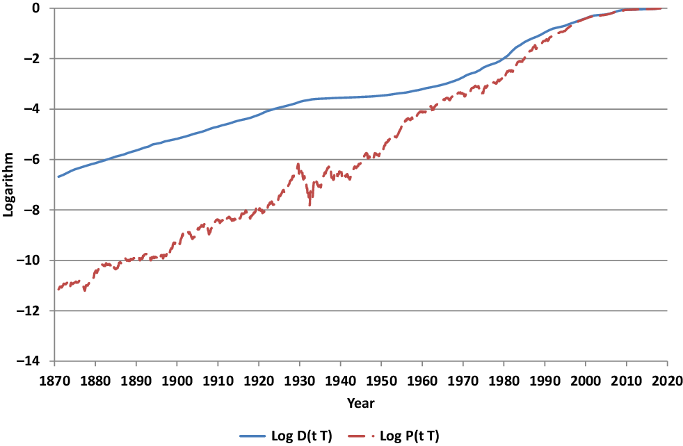
Figure 4 Logarithms of values of savings bond and fair zero coupon bond.

Figure 5 Values of benchmarked savings bond and benchmarked fair zero coupon bond.
As pointed out previously and shown in Baldeaux et al. (Reference Baldeaux, Grasselli and Platen2015) and (Reference Baldeaux, Ignatieva and Platen2018), an equivalent risk-neutral probability measure is unlikely to exist for any realistic model for the US market. This is also consistent with the practice of financial planning. Financial planning recommends to invest at young age in the equity market and to shift wealth into fixed income securities closer to retirement. This type of strategy is widely acknowledged to be more efficient than investing all wealth in a savings bond, which represents the classical risk-neutral strategy for obtaining bond payoffs at maturity. The BA allows us to make the financial planning strategy rigorous, and both the savings account and a less-expensive fair bond are possible without creating economically meaningful arbitrage. Based on the absence of an equivalent risk-neutral probability measure, this paper provides the theoretical reasoning for the financial planning strategy. Moreover, it will quantify rigorously such a strategy under the assumption of a stylized model. The absence of an equivalent risk-neutral probability measure is also consistent with the existence of target date funds, which pay cash at maturity and have a glide path that invests early on in risky securities. Also, this glide path can be made rigorous in a similar manner as described below for the fair zero coupon bond.
5.2 Fair zero coupon bond
Under real-world valuation, the time t value of the fair zero coupon bond price with maturity date T is denoted by
 \begin{equation} P(t,T) = S^*_t\,E_t\left( \frac{1}{S^*_T}\right) , \end{equation}
and results from the real-world valuation formula (6), see also (8). It provides the minimal possible price for a self-financing portfolio that replicates $\$1$
at maturity T. The underlying assets involved are the benchmark (here the S
$\$1$
at maturity T. The underlying assets involved are the benchmark (here the S $\&$
P500 total return index) and the savings account of the domestic currency, here the US dollar. Both securities will appear in the corresponding hedge portfolio, which shall replicate at maturity the payoff of one dollar.
$\&$
P500 total return index) and the savings account of the domestic currency, here the US dollar. Both securities will appear in the corresponding hedge portfolio, which shall replicate at maturity the payoff of one dollar.
To calculate the value of a fair zero coupon bond, one has to compute the real-world conditional expectation in (12). For this calculation, one needs to employ a model for the real-world distribution of the random variable $(S^*_T)^{-1}$
. Any model that models the benchmarked savings account as a strict supermartingale will value the above benchmarked fair zero coupon bond less expensively than the corresponding benchmarked savings bond. Figure 5 displays, additionally to the benchmarked savings bond, the value of a benchmarked fair zero coupon bond, which will be derived below, under a respective model. One notes the significantly lower initial value of the benchmarked fair zero coupon bond. Also visually, its benchmarked value seems to appear as a reasonable forecast of its future benchmarked values, reflecting its martingale property. In Figure 4, the logarithm of the fair zero coupon bond is shown together with the logarithm of the savings bond value. The fair zero coupon bond price at time t is computed using (18), where for the model we explain later on the parameter values are given in (17) and D(t,T) in (11). One notes that the fair zero coupon bond appears to follow early on essentially the benchmark for many years and glides later on more and more towards the savings account. The strategy that delivers this hedging portfolio will be discussed in detail below.
$(S^*_T)^{-1}$
. Any model that models the benchmarked savings account as a strict supermartingale will value the above benchmarked fair zero coupon bond less expensively than the corresponding benchmarked savings bond. Figure 5 displays, additionally to the benchmarked savings bond, the value of a benchmarked fair zero coupon bond, which will be derived below, under a respective model. One notes the significantly lower initial value of the benchmarked fair zero coupon bond. Also visually, its benchmarked value seems to appear as a reasonable forecast of its future benchmarked values, reflecting its martingale property. In Figure 4, the logarithm of the fair zero coupon bond is shown together with the logarithm of the savings bond value. The fair zero coupon bond price at time t is computed using (18), where for the model we explain later on the parameter values are given in (17) and D(t,T) in (11). One notes that the fair zero coupon bond appears to follow early on essentially the benchmark for many years and glides later on more and more towards the savings account. The strategy that delivers this hedging portfolio will be discussed in detail below.
We interpret the value of the savings bond as the one obtained by formal risk-neutral valuation. As shown in relation (10), this value is greater than or equal to that of the fair zero coupon bond. For readers who want to have some economic explanation for the observed value difference, one could argue that the savings bond gives the holder the right to liquidate the contract at any time without costs. On the other hand, a fair zero coupon bond is akin to a term deposit without the right to access the assets before maturity. One could say that the savings bond carries a “liquidity premium” on top of the value for the fair zero coupon bond. Under the classical no-arbitrage paradigm, with its Law of One Price (see e.g. Taylor Reference Taylor2002), there is only one and the same value process possible for both instruments, which is that of the savings bond. The BA opens with its real-world valuation concept the possibility to model costs for early liquidation of financial instruments. The fair zero coupon bond is the least liquid instrument that delivers the bond payoff, and therefore, the least expensive zero coupon bond. The savings bond is more liquid and, therefore, more expensive.
5.3 Fair zero coupon bond for the minimal market model
The benchmarked fair zero coupon value at time $t\in [0,T]$
is the best forecast of its benchmarked payoff
$t\in [0,T]$
is the best forecast of its benchmarked payoff ${\hat{S}}^0_T = (S^*_T)^{-1}$
. It provides the minimal self-financing portfolio value process that hedges this benchmarked contingent claim. To facilitate a tractable evaluation of a fair zero coupon bond, we employ a continuous time model for the benchmarked savings account that models it as a strict supermartingale. The inverse of the benchmarked savings account is the discounted numéraire portfolio
${\hat{S}}^0_T = (S^*_T)^{-1}$
. It provides the minimal self-financing portfolio value process that hedges this benchmarked contingent claim. To facilitate a tractable evaluation of a fair zero coupon bond, we employ a continuous time model for the benchmarked savings account that models it as a strict supermartingale. The inverse of the benchmarked savings account is the discounted numéraire portfolio ${\bar{S}}^*_t=\frac{S^*_t}{S^0_t} = ({\hat{S}}^0_t)^{-1}$
. In the illustrative example we present, it is the discounted S
${\bar{S}}^*_t=\frac{S^*_t}{S^0_t} = ({\hat{S}}^0_t)^{-1}$
. In the illustrative example we present, it is the discounted S $\&$
P500, which, as discounted numéraire portfolio, satisfies in a continuous market model the stochastic differential equation (SDE)
$\&$
P500, which, as discounted numéraire portfolio, satisfies in a continuous market model the stochastic differential equation (SDE)
 \begin{equation} d\, {\bar{S}}^*_t =\alpha_t\,dt + \sqrt{{\bar{S}}^*_t\,\alpha_t} \,dW_t, \end{equation}
for $t\ge 0$
with
$t\ge 0$
with ${\bar{S}}^*_0 >0$
, see Platen & Heath (Reference Platen and Heath2010) Formula (13.1.6). Here
${\bar{S}}^*_0 >0$
, see Platen & Heath (Reference Platen and Heath2010) Formula (13.1.6). Here $W=\{W_t, t\ge 0\}$
is a Wiener process, and
$W=\{W_t, t\ge 0\}$
is a Wiener process, and $\alpha=\{\alpha_t,t\ge 0\}$
is a strictly positive process, which models the trend
$\alpha=\{\alpha_t,t\ge 0\}$
is a strictly positive process, which models the trend $\alpha_t={\bar{S}}^*_t \theta^2_t$
of
$\alpha_t={\bar{S}}^*_t \theta^2_t$
of ${\bar{S}}^*_t$
, with
${\bar{S}}^*_t$
, with $\theta_t$
denoting the market price of risk. Since in (13)
$\theta_t$
denoting the market price of risk. Since in (13) $\alpha_t$
can be a rather general stochastic process, the parametrisation of the SDE (13) does so far not constitute a model. For constant market price of risk, one obtains the Black-Scholes model, which has been the standard market model. In the long term, it yields a benchmarked savings account that is a true martingale and is, therefore, having an equivalent risk-neutral probability measure, which appears to be unrealistic for long-term modelling.
$\alpha_t$
can be a rather general stochastic process, the parametrisation of the SDE (13) does so far not constitute a model. For constant market price of risk, one obtains the Black-Scholes model, which has been the standard market model. In the long term, it yields a benchmarked savings account that is a true martingale and is, therefore, having an equivalent risk-neutral probability measure, which appears to be unrealistic for long-term modelling.
The trend or drift in the SDE (13) can be interpreted economically as a measure for the discounted fundamental value of wealth generated per unit of time by the underlying economy. To construct a respective model, we assume in the following that the drift of the discounted S $\&$
P500 total return index grows exponentially with a constant net growth rate
$\&$
P500 total return index grows exponentially with a constant net growth rate $\eta > 0$
. At time t, the drift of the discounted S
$\eta > 0$
. At time t, the drift of the discounted S $\&$
P500 total return index
$\&$
P500 total return index ${\bar{S}}^*_t$
is then modelled by the exponential function
${\bar{S}}^*_t$
is then modelled by the exponential function
 \begin{equation}\alpha_t= {\alpha}\,\exp\{\eta\,t\}.\end{equation}
This yields the stylized version of the minimal market model (MMM), see Platen (Reference Platen2001, Reference Platen2002a), which emerges from (13). We know explicitly the transition density of the resulting time-transformed squared Bessel process of dimension four, ${\bar{S}}^*$
, see Revuz & Yor (Reference Revuz and Yor1999). It equals
${\bar{S}}^*$
, see Revuz & Yor (Reference Revuz and Yor1999). It equals
 \begin{equation}p_{{\bar{S}}^*}(t, x_t , {\bar{T}} , x_{\bar{T}} ) = \frac{1}{2(\varphi_{\bar{T}} - \varphi_t )} \sqrt{\frac{x_{\bar{T}}}{x_t}} \exp \left( -\frac{x_t + x_{\bar{T}}}{2(\varphi_{\bar{T}} - \varphi_t )} \right) I_1 \left( \frac{\sqrt{x_t x_{\bar{T}}}}{\varphi_{\bar{T}} - \varphi_t} \right) ,\end{equation}
where
 \begin{equation} \varphi_t = \frac{1}{4\eta }\alpha (\exp(\eta t)-1)\end{equation}
is also the quadratic variation of $ \sqrt{{\bar{S}}^*} $
. The corresponding distribution function is that of a non-central chi-squared random variable with four degrees of freedom and non-centrality parameter
$ \sqrt{{\bar{S}}^*} $
. The corresponding distribution function is that of a non-central chi-squared random variable with four degrees of freedom and non-centrality parameter $x_t/(\varphi_T - \varphi_t)$
.
$x_t/(\varphi_T - \varphi_t)$
.
Using the above transition density function, we apply standard maximum likelihood estimation to monthly data for the discounted S $\&$
P500 total return index over the period from January 1871 to January 1932, giving the following estimates of the parameters
$\&$
P500 total return index over the period from January 1871 to January 1932, giving the following estimates of the parameters $\alpha$
and
$\alpha$
and $\eta$
,
$\eta$
,
 \begin{align}\alpha &= 0.005860\, (0.000613 ),\nonumber \\[5pt] \eta &= 0.049496 \, (0.002968) ,\end{align}
where the standard errors are shown in brackets. In Appendix A, we explain the estimation method used and supply parameter estimates over other periods, where it is evident that the estimates are consistent over time.
These estimates for the net growth rate $\eta$
are consistent with estimates from various other sources in the literature, where the net growth rate of the US equity market during the last century has been estimated at about 5%; see for instance Dimson et al. (Reference Dimson, Marsh and Staunton2002).
$\eta$
are consistent with estimates from various other sources in the literature, where the net growth rate of the US equity market during the last century has been estimated at about 5%; see for instance Dimson et al. (Reference Dimson, Marsh and Staunton2002).
Under the stylized MMM, the explicitly known transition density of the discounted numéraire portfolio ${\bar{S}}^*_t$
yields for the fair zero coupon bond price by (12) the explicit formula
${\bar{S}}^*_t$
yields for the fair zero coupon bond price by (12) the explicit formula
 \begin{equation} P(t,T) = D(t,T)\left( 1-\exp\left\{-\frac{2\,\eta\,{\bar{S}}^*_t} {\alpha\,(\exp\{\eta\,T\} - \exp\{\eta\,t\})} \right\}\right) \end{equation}
for $t \in [0,T)$
, which has been first pointed out in Platen (Reference Platen2002b). Figure 5 displays with the lower graph the trajectory of the benchmarked fair zero coupon bond value with maturity T in May 2018. By (18), the value of the benchmarked fair zero coupon bond remains always below that of the benchmarked savings bond, where we interpret the latter as the formally obtained risk-neutral zero coupon bond value. The fair zero coupon bond value provides the minimal portfolio process for hedging the given payoff under the assumed MMM. Other benchmarked portfolios with the same payoff need to form strict supermartingales and, therefore, yield higher value processes. One such example is given by the benchmarked savings bond. Recall that the benchmarked fair zero coupon bond is a martingale. It is minimal among the supermartingales that represent benchmarked replicating self-financing portfolios and pays one dollar at maturity.
$t \in [0,T)$
, which has been first pointed out in Platen (Reference Platen2002b). Figure 5 displays with the lower graph the trajectory of the benchmarked fair zero coupon bond value with maturity T in May 2018. By (18), the value of the benchmarked fair zero coupon bond remains always below that of the benchmarked savings bond, where we interpret the latter as the formally obtained risk-neutral zero coupon bond value. The fair zero coupon bond value provides the minimal portfolio process for hedging the given payoff under the assumed MMM. Other benchmarked portfolios with the same payoff need to form strict supermartingales and, therefore, yield higher value processes. One such example is given by the benchmarked savings bond. Recall that the benchmarked fair zero coupon bond is a martingale. It is minimal among the supermartingales that represent benchmarked replicating self-financing portfolios and pays one dollar at maturity.
5.4 Comparison of values of savings and fair zero coupon bond
In this subsection, we compare the values of the savings bond and the zero coupon bond.
Figure 6 exhibits with its upper graph the trajectory of the savings bond and with its lower graph that of the zero coupon bond in US dollar denomination. Closer to maturity, the fair zero coupon bond’s value merges asymptotically with the savings bond value. Both self-financing portfolios replicate the payoff at maturity. Most important is the observation that they start with significantly different initial values. The fair zero coupon bond exploits the strict supermartingale property of the benchmarked savings account by targeting its value at maturity, whereas the savings bond ignores it. Two self-financing replicating portfolios are displayed in Figure 6. Such a situation, where two self-financing portfolios replicate the same contingent claim, is impossible under the classical no-arbitrage paradigm. However, under the BA this is a natural situation.

Figure 6 Values of savings bond and fair zero coupon bond.
In the above example for the parameters estimated during the period from January 1871 to January 1932, the savings bond with maturity in May 2018 has in January 1932 a value of $D(0,T) = S^0_0/S^0_T \approx \$0.026085 $
, where we have substituted from our data set the values
$D(0,T) = S^0_0/S^0_T \approx \$0.026085 $
, where we have substituted from our data set the values $S^0_0 = 20.809541 $
and
$S^0_0 = 20.809541 $
and $S^0_T = 797.7633 $
. The fair zero coupon bond is far less expensive and valued at only
$S^0_T = 797.7633 $
. The fair zero coupon bond is far less expensive and valued at only $P(0,T) = D(0,T) (1-\exp (-2\eta {\bar{S}}^*_0 / \{ \alpha (\exp(\eta T) - 1)\} \approx \$0.000657 $
, where we have substituted the value of
$P(0,T) = D(0,T) (1-\exp (-2\eta {\bar{S}}^*_0 / \{ \alpha (\exp(\eta T) - 1)\} \approx \$0.000657 $
, where we have substituted the value of ${\bar{S}}^*_0$
, inferred from the values of
${\bar{S}}^*_0$
, inferred from the values of $S^0_0$
and
$S^0_0$
and $S^*_0 = 45.498333 $
in our data set, and the values of
$S^*_0 = 45.498333 $
in our data set, and the values of $\alpha$
and
$\alpha$
and $\eta$
given in (17). The fair zero coupon bond with term to maturity of more than 80 years costs here less than 3% of the savings bond. This reveals a substantial premium in the value of the savings bond.
$\eta$
given in (17). The fair zero coupon bond with term to maturity of more than 80 years costs here less than 3% of the savings bond. This reveals a substantial premium in the value of the savings bond.
Of course, usually one has to deal with shorter terms to maturity in annuities. Therefore, we repeated with the estimated parameters the study for all possible zero coupon bonds that cover a period of 10, 15, 20, 25, 30 and 35 years from initiation until maturity that fall into the period starting in January 1932 and ending in May 2018. Table 1 displays the average percentage value of the risk-neutral over the fair bond. One notes that for a 25-year bond, one saves on average about 20% of the risk-neutral value, which is a substantial part and typical for pension products.
Table 1. Mean values of zero coupon bonds of prescribed terms to maturity whose start and end dates lie between January 1932 and May 2018.

By describing below the hedging strategy that generates the fair zero coupon bond, we propose a realistic way of changing industry practice from the classical risk-neutral production to the less expensive benchmark production.
5.5 Hedging of a fair zero coupon bond
The benefits of the proposed benchmark production methodology can be harvested if the respective hedging strategy is followed. The hedging strategy by which this is achieved follows under the MMM from the explicit fair zero coupon bond valuation formula (13). At the time, $t \in [0,T)$
the corresponding theoretical number of units of the S
$t \in [0,T)$
the corresponding theoretical number of units of the S $\&$
P500 to be held in the hedge portfolio follows, similar to the well-known Black-Scholes delta hedge ratio, as partial derivative of the bond value with respect to the underlying, and is given by the formula
$\&$
P500 to be held in the hedge portfolio follows, similar to the well-known Black-Scholes delta hedge ratio, as partial derivative of the bond value with respect to the underlying, and is given by the formula
 \begin{eqnarray} \delta^*_t &=& \frac{\partial {\bar{P}}(t,T)}{\partial {\bar{S}}^*_t} \nonumber \\[5pt] &=& D(0,T)\, \exp\left\{\frac{- 2\,\eta\,{\bar{S}}^*_t} {\alpha\,(\exp\{\eta\,T\} - \exp\{\eta\,t\})} \right\} \, \frac{2\,\eta} {\alpha\,(\exp\{\eta\,T\} - \exp\{\eta\,t\})}. \end{eqnarray}
Here D(0,T) is the respective value of the savings bond.
One may argue that transaction costs may play a role and could make the hedge critically more expensive than shown. Here we argue that the hedger will sell the index when it is just reaching new high levels, where most investors are buyers, and will buy the index when it reaches new relatively low values, where many investors typically sell the index. This hedging strategy will have a stabilising effect on the financial market if it is pursued by many institutions. Note that brokers often waive transaction costs for those who supply liquidity to the market as done by the strategy. In practice, implementing the hedging strategy is achieved straightforwardly using buy and sell limit orders which are permitted on most financial exchanges.
The resulting fraction of wealth to be held at time t in the S $\&$
P500, as it evolves for the given example of zero coupon bond valuation from January 1932 to maturity, is shown in Figure 7. The remaining wealth is always invested in the savings account.
$\&$
P500, as it evolves for the given example of zero coupon bond valuation from January 1932 to maturity, is shown in Figure 7. The remaining wealth is always invested in the savings account.
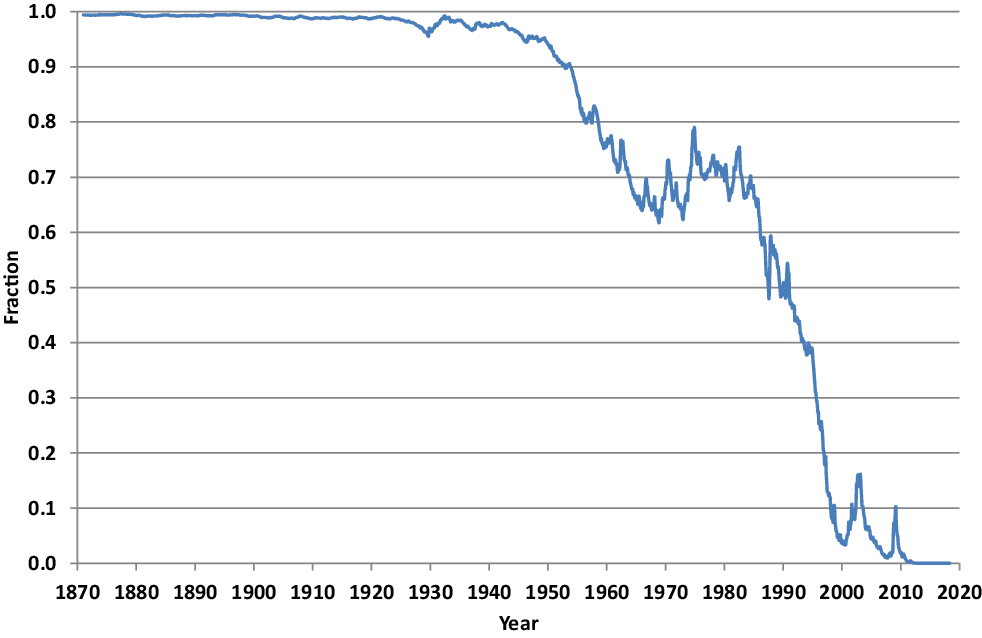
Figure 7 Fraction of wealth invested in the S $\&$
P500.
$\&$
P500.
To demonstrate how realistic the hedge of the fair zero coupon bond payoff is for the given delta under the stylized MMM with monthly reallocation, a self-financing hedge portfolio is formed. The delta hedge is performed, where the self-financing hedge portfolio starts in January 1932, which ensures that the hedge simulations employing the fitted parameters in (17) are out-of-sample. Each month, the fraction invested in the S $\&$
P500 is adjusted in a self-financing manner according to the above prescription. The resulting benchmarked profit and loss for this delta hedge turns out to be very small and is visualized in Figure 8. The maximum absolute benchmarked profit and loss amounts only to about 0.00000061. This benchmarked profit and loss is so small that the resulting hedge portfolio, when plotted additionally in Figure 6, would be visually indistinguishable from the path of the already displayed fair zero coupon bond price process. Dollar values of the self-financing hedge portfolio for the fair zero coupon bond and the savings bond are shown in Figure 9, where it is evident that the self-financing portfolio replicates 95% of the face value of the bond but employs less than 3% of the initial capital. One may argue that this represents only one hedge simulation. Therefore, we employ 10, 15, 20 and 25 year fair bonds that fit from initiation until maturity into the period from January 1932 until May 2018 and perform analogous hedge simulations. In Table 2, we report in US dollars the average profits and losses with respective standard deviations, where for a 25-year fair zero coupon bond the hedge losses at maturity average 2.26% of the face value while the initial hedge portfolio is 20% less expensive than the savings bond. With a more refined model and more frequent hedging, one can expect to reduce the hedge error.
$\&$
P500 is adjusted in a self-financing manner according to the above prescription. The resulting benchmarked profit and loss for this delta hedge turns out to be very small and is visualized in Figure 8. The maximum absolute benchmarked profit and loss amounts only to about 0.00000061. This benchmarked profit and loss is so small that the resulting hedge portfolio, when plotted additionally in Figure 6, would be visually indistinguishable from the path of the already displayed fair zero coupon bond price process. Dollar values of the self-financing hedge portfolio for the fair zero coupon bond and the savings bond are shown in Figure 9, where it is evident that the self-financing portfolio replicates 95% of the face value of the bond but employs less than 3% of the initial capital. One may argue that this represents only one hedge simulation. Therefore, we employ 10, 15, 20 and 25 year fair bonds that fit from initiation until maturity into the period from January 1932 until May 2018 and perform analogous hedge simulations. In Table 2, we report in US dollars the average profits and losses with respective standard deviations, where for a 25-year fair zero coupon bond the hedge losses at maturity average 2.26% of the face value while the initial hedge portfolio is 20% less expensive than the savings bond. With a more refined model and more frequent hedging, one can expect to reduce the hedge error.
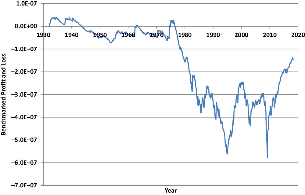
Figure 8 Benchmarked profit and loss.

Figure 9 Hedge portfolios of zero coupon bonds and profit and loss.
Table 2. Means and standard deviations of profits and losses on hedge at maturities of zero coupon bonds having various terms to maturity. (Negative P&Ls indicate losses).
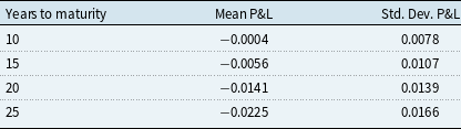
The above example and hedge simulations demonstrate the principle findings that a hedge portfolio can generate a fair zero coupon bond value process by investing long only in a dynamic hedge in the S $\&$
P500 and the savings account. The resulting hedge portfolio is for long-term maturities significantly less expensive than the corresponding savings bond. Moreover, as can be seen in Figure 4, the hedge portfolio can initially significantly fluctuate, as it did around 1930 during the Great Depression. Close to maturity, the hedge portfolio cannot be significantly affected by any equity market meltdown, as was the case in our illustrative example during the 2007–2008 financial crisis. This protection against a major draw down close to the retirement date is what financial planning aims to avoid intuitively. It is here made rigorous by following the dynamic allocation strategy (19).
$\&$
P500 and the savings account. The resulting hedge portfolio is for long-term maturities significantly less expensive than the corresponding savings bond. Moreover, as can be seen in Figure 4, the hedge portfolio can initially significantly fluctuate, as it did around 1930 during the Great Depression. Close to maturity, the hedge portfolio cannot be significantly affected by any equity market meltdown, as was the case in our illustrative example during the 2007–2008 financial crisis. This protection against a major draw down close to the retirement date is what financial planning aims to avoid intuitively. It is here made rigorous by following the dynamic allocation strategy (19).
In a similar manner as above described, one can value and produce less expensively other long-term contingent claims including equity-linked payoffs that are typical for variable annuities or life insurance and pension payoffs. Below, we will illustrate the proposed valuation and production methodology for annuities.
In summary, by shifting the valuation paradigm from classical risk-neutral to real-world valuation, we suggest to produce more cost efficiently long-term payoffs.
5.6 Stylized long-term cash-linked annuity
Consider now a stylized example that aims to illustrate valuation and production under the BA in the context of a basic stylized annuity. Here we assume that the savings account and total return index account commence with $\$ $
1 at the date
$\$ $
1 at the date $t_0$
. Consider annuities sold at some time
$t_0$
. Consider annuities sold at some time $t_0$
to K policy holders that pay an indexed number of units of the savings account per year at the beginning of each year where they provide a payoff. We denote by G the set of dates on which the annuity provides a payoff. Furthermore,
$t_0$
to K policy holders that pay an indexed number of units of the savings account per year at the beginning of each year where they provide a payoff. We denote by G the set of dates on which the annuity provides a payoff. Furthermore, $\tau^{(k)}$
is a random variable equal to the time at which the k-th policy holder dies, for
$\tau^{(k)}$
is a random variable equal to the time at which the k-th policy holder dies, for $k=1,2,\ldots , K$
. The payoff at time
$k=1,2,\ldots , K$
. The payoff at time $T\in G$
in respect of the k-th policy holder is
$T\in G$
in respect of the k-th policy holder is
 \begin{equation}MI_T\times \frac{S^0_T}{S^0_{t_0}} \times 1_{\tau^{(k)}>T }.\end{equation}
The indexed number $MI_T$
of units at time T is prescribed as
$MI_T$
of units at time T is prescribed as
 \begin{equation}MI_T = \frac{\xi }{\epsilon +\sum_{k=1}^K 1_{\tau^{(k)}>T }},\, \mathrm{for}\, {\epsilon ,\, }\xi>0.\end{equation}
This type of payoff is likely to account well in the long-run for the effect of inflation if the average US interest rate is, as it was during the last century, on average about 1% above the US average inflation rate, as demonstrated in Dimson et al. (Reference Dimson, Marsh and Staunton2002). Additionally, we assume that there is an asset management fee payable as an annuity whose payoff at time T equals, for the entire portfolio, $\epsilon MI_T\times \frac{S^0_T}{S^0_{t_0}}$
,
$\epsilon MI_T\times \frac{S^0_T}{S^0_{t_0}}$
, $\epsilon >0$
.
$\epsilon >0$
.
In our valuation, the interest rate will not play any role, and we cover the case that the interest rate is stochastic and not known to us. Also, since the portfolio of annuities has at time $T\in G$
the aggregate payoff
$T\in G$
the aggregate payoff
 \begin{equation}\epsilon MI_T\times \frac{S^0_T}{S^0_{t_0}} + \sum_{k=1}^K \bigg\{ MI_T\times \frac{S^0_T}{S^0_{t_0}} \times 1_{\tau^{(k)}>T } \bigg\} = \xi \frac{S^0_T}{S^0_{t_0}} ,\end{equation}
the mortality rate will play no role in our valuation and we cover the case that the mortality rate is stochastic and not known to us. Of course, this setup is idealized but also reasonable for demonstrating the effect of real-world valuation for annuities. From the modelling point of view, we avoid here deliberately the modelling of the interest rate and the mortality rate. Furthermore, the payoff is fully replicable.
To use the available historical data efficiently, let us place our discussion in the past and consider a cohort of K persons who reached the age of 25 in January 1932. The K persons purchase some annuity which pays, from the age of 65 to the beginning of the age of 110, at the beginning of each year T the indexed number of units $MI_T$
of the savings account. In the case when the person may have passed away before reaching the age of 110 in 2017, the payments that would have otherwise been made revert to the asset pool backing the annuity portfolio. Obviously, the longer surviving individuals receive more savings account units in later years than in earlier years, which is important because they may need more age care. Since in this setting there is no mortality risk or interest rate risk involved in the given payoff stream, classical risk-neutral valuation would value this annuity portfolio at time t as
$MI_T$
of the savings account. In the case when the person may have passed away before reaching the age of 110 in 2017, the payments that would have otherwise been made revert to the asset pool backing the annuity portfolio. Obviously, the longer surviving individuals receive more savings account units in later years than in earlier years, which is important because they may need more age care. Since in this setting there is no mortality risk or interest rate risk involved in the given payoff stream, classical risk-neutral valuation would value this annuity portfolio at time t as
 \begin{equation}V^{\textrm{RN}}_t = \sum_{T\in G} S^0_t E_t \left( \xi \frac{S^0_T/S^0_{t_0}}{S^0_T} \right) = 45\times \xi \frac{S^0_t}{S^0_{t_0}}\end{equation}
for the set of 45 possible payment dates $G = \{\textrm{Jan }1972, \textrm{Jan }1973,\dots, \textrm{Jan }2016\}$
. Thus for any date t during the period from January 1932 until December 1971, classical risk-neutral valuation would always value this annuity portfolio as being equal to
$G = \{\textrm{Jan }1972, \textrm{Jan }1973,\dots, \textrm{Jan }2016\}$
. Thus for any date t during the period from January 1932 until December 1971, classical risk-neutral valuation would always value this annuity portfolio as being equal to $45\xi$
units of the savings account. This is exactly the number of units of the savings account that have to be paid out by the annuity over the 45 years from 1972 until 2017. This means the annuity has the discounted risk-neutral value
$45\xi$
units of the savings account. This is exactly the number of units of the savings account that have to be paid out by the annuity over the 45 years from 1972 until 2017. This means the annuity has the discounted risk-neutral value
 \begin{equation} \bar{V}^{\textrm{RN}}_t=\frac{V^{\textrm{RN}}_t}{S^0_t}=45\xi\end{equation}
for all times $t \in \{\textrm{Jan }1932, \textrm{Feb }1932,\dots, \textrm{Dec }1971\}$
before the possible payment dates start. Note that the purchasing time does not play here a role.
$t \in \{\textrm{Jan }1932, \textrm{Feb }1932,\dots, \textrm{Dec }1971\}$
before the possible payment dates start. Note that the purchasing time does not play here a role.
As we will show in the following sections, when valuing such an annuity under the BA it will be less expensive than suggested by the above classical risk-neutral value. This example aims to illustrate again that significant amounts can be saved.
For the later described model and fitted parameters, Figure 10 shows the discounted value of the proposed less-expensive annuity portfolio (denominated in units of the savings account, with $\xi=1$
), as a function of the purchasing time t. One notes that the time of purchase plays a significant role. Over the years, the discounted fair annuity becomes more expensive. The value of the fair annuity remains always below that of the corresponding risk-neutral value. It is ranging from about 10% of the risk-neutral value in January 1932 to about 89% of the risk-neutral value in December 1971. This means someone who starts at the beginning of her or his working life to prepare for retirement can enjoy benefits about eight times greater than those delivered from a later start when it is close to retirement. Note that the typical compounding effect in a savings account does not matter in this example because the value of the annuity and its payments are denominated in units of the savings account. It is the application of the BA that unleashes the remarkable cost saving due to the supermartingale property of the benchmarked savings account.
$\xi=1$
), as a function of the purchasing time t. One notes that the time of purchase plays a significant role. Over the years, the discounted fair annuity becomes more expensive. The value of the fair annuity remains always below that of the corresponding risk-neutral value. It is ranging from about 10% of the risk-neutral value in January 1932 to about 89% of the risk-neutral value in December 1971. This means someone who starts at the beginning of her or his working life to prepare for retirement can enjoy benefits about eight times greater than those delivered from a later start when it is close to retirement. Note that the typical compounding effect in a savings account does not matter in this example because the value of the annuity and its payments are denominated in units of the savings account. It is the application of the BA that unleashes the remarkable cost saving due to the supermartingale property of the benchmarked savings account.

Figure 10 Savings account discounted price of the annuity during the period from January 1932 until December 1971 which provides annual payments from January 1972 until January 2016.
To demonstrate that the above effect holds independently from the period entered, we repeat for analogous contracts the calculations for all possible start dates within the period from January 1871 until January 1932. We show in Table 3 the mean percentage saving by using the proposed benchmark methodology and the standard deviation for this estimate.
Table 3. Comparison of discounted values of deferred annuities paying one dollar per annum for forty five years, commencing in 40 years’ time, over all monthly start dates in the period January 1871 to January 1932.
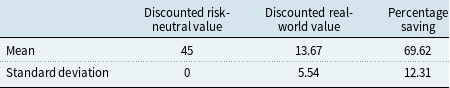
5.7 Long-term cash-linked annuity
We describe now in detail the calculations for the stylized long-term annuity that we introduced in section 5.6. As proxy for the NP, we use the S&P500. The subset of the monthly S $\&$
P500 time series used for fitting the parameters in (17) starts at January 1871 and ends at January 1932. The real-world valuation formula, given in (6), captures at time t the fair value of one unit of the savings account at time T, see (11) and (13), via the expression
$\&$
P500 time series used for fitting the parameters in (17) starts at January 1871 and ends at January 1932. The real-world valuation formula, given in (6), captures at time t the fair value of one unit of the savings account at time T, see (11) and (13), via the expression
 \begin{equation} S^*_t E_t\Big(\frac{S^0_T}{S^*_T}\Big)=S^0_t E_t\Big(\frac{{\bar S}^*_t}{{\bar S}^*_T}\Big) = S^0_t\left( 1-\exp\left\{-\frac{2\,\eta\,{\bar{S}}^*_t} {\alpha\,(\exp\{\eta\,T\} - \exp\{\eta\,t\})} \right\}\right) .\end{equation}
Consequently, the discounted real-world value of the annuity portfolio at the time $t \in \{\textrm{Jan }1932, \textrm{Feb }$ $1932, \dots, \textrm{Dec }1971\}$
equals
$1932, \dots, \textrm{Dec }1971\}$
equals
 \begin{equation} {\bar{V}}^{\textrm{RW}}_t=\xi \sum_{T \in G}\frac{S^*_t}{S^0_t} E_t\Big(\frac{S^0_T}{S^*_T}\Big)=\xi \sum_{T\in G}\left( 1-\exp\left\{-\frac{2\,\eta\,{\bar{S}}^*_t} {\alpha\,(\exp\{\eta\,T\} - \exp\{\eta\,t\})} \right\}\right)\end{equation}
for the set of payment dates $G=\{\textrm{Jan }1972,\textrm{Jan }1973,\dots,\textrm{Jan }2016\}$
.
$G=\{\textrm{Jan }1972,\textrm{Jan }1973,\dots,\textrm{Jan }2016\}$
.
The payoff stream of the fair annuity needs to be hedged, generating only a small benchmarked profit and loss or hedge error of similar size as demonstrated in the previous section, where we considered a single fair zero coupon bond. Now we have a portfolio of bonds that pays units of the savings account at their maturities. With these assumptions, we obtain the remarkable results shown in Figure 10 and Table 3, with $\xi=1$
.
$\xi=1$
.
5.8 Long-term mortality and equity-linked annuities with mortality and cash-linked guarantees
To demonstrate that the proposed methodology works also well for equity-linked annuities, consider now a stylized example that aims to illustrate valuation and hedging under the BA in the context of annuities that offer optional guarantees, as is typical in variable annuities. We may assume also here that interest rates are stochastic because this will not affect our proposed valuation and production. Consider an annuity that pays to a policy holder at times $T\in G$
until maturity the greater value of
$T\in G$
until maturity the greater value of $MI_T\times \exp(\eta(T-t_0))$
units of the savings account and
$MI_T\times \exp(\eta(T-t_0))$
units of the savings account and $MI_T$
units of the S
$MI_T$
units of the S $\&$
P500 total return index account per year at the beginning of each year while the policy holder is alive. Here we assume that the potential savings account or the total return index account payments commence with $1 at the date
$\&$
P500 total return index account per year at the beginning of each year while the policy holder is alive. Here we assume that the potential savings account or the total return index account payments commence with $1 at the date $t_0$
of purchasing the annuity. As in the previous example, we assume that there is an asset management fee payable as annuity whose payoff at time T is the same as for a living policy holder.
$t_0$
of purchasing the annuity. As in the previous example, we assume that there is an asset management fee payable as annuity whose payoff at time T is the same as for a living policy holder.
The real-world value at time t of one of the above payments at the future time T is given by
 \begin{equation}V^{\textrm{RW}}_{t,T} = S_t^* E_t\left( \frac{1}{S_T^*}\max \Big( \frac{S^*_T}{S^*_{t_0}}, \frac{S^0_T\exp(\eta(T-t_0))}{S^0_{t_0}} \Big) \right)\end{equation}
which rearranges as
 \begin{align}V^{\textrm{RW}}_{t,T} &= \frac{S^0_t}{S^0_{t_0}} E_t\left(\max \Big( \frac{{\bar{S}}^*_{t}}{{\bar{S}}^*_{t_0}} , \frac{{\bar{S}}^*_{t}\exp(\eta(T-t_0))}{{\bar{S}}^*_T} \Big)\right)\\[3pt]\notag&= \frac{{{S}}^*_{t}}{{{S}}^*_{t_0}}+ \frac{S^0_t}{S^0_{t_0}} \exp(\eta(T-t_0)) E_t\left(\Big( \frac{{\bar{S}}^*_{t}}{{\bar{S}}^*_T} - \frac{{\bar{S}}^*_{t}}{{\bar{S}}^*_{t_0}\exp(\eta(T-t_0))} \Big)^{+}\right) . \end{align}
This rearrangment shows that today’s value is the sum of an equity-linked component and an equity index put option component. As in the previous example, neither the interest rate nor the mortality rate plays a role in the valuation formula.
We recall that the discounted index value is non-central chi-squared distributed, which allows us to use the following lemma to compute the real-world value of the above guarantee.
Lemma 1. Let U be a non-central chi-squared random variable with four degrees of freedom and non-centrality parameter $\lambda>0$
. Then, the following expectations hold:
$\lambda>0$
. Then, the following expectations hold:
 \begin{align} E\left( \frac{\lambda}{U} \right) &= 1-\exp (-\lambda /2)\end{align}
 \begin{align} E\left( \frac{\lambda}{U} 1_{U< x}\right) &= \chi^2_{0,\lambda }(x) - \exp (-\lambda /2)\end{align}
 \begin{align} E\left( \frac{\lambda}{U} 1_{U\ge x}\right) &= 1-\chi^2_{0,\lambda }(x),\end{align}
where $\chi^2_{\nu,\lambda}(x)$
denotes the cumulative distribution function of a non-central chi-squared random variable having
$\chi^2_{\nu,\lambda}(x)$
denotes the cumulative distribution function of a non-central chi-squared random variable having $\nu$
degrees of freedom and non-centrality parameter
$\nu$
degrees of freedom and non-centrality parameter $\lambda$
.
$\lambda$
.
The proof of this lemma is given in Appendix B.
Furthermore, we mention the following result which we prove in Appendix C.
Corollary 2. For a discounted numéraire portfolio process ${\bar{S}}^*$
, obeying the SDE (13), we have the expectations
${\bar{S}}^*$
, obeying the SDE (13), we have the expectations
 \begin{align} E_t\left( \frac{{\bar{S}}^*_{t}}{{\bar{S}}^*_T} \right) &= 1-\exp (-\lambda (t,T) /2)\end{align}
 \begin{align} E_t\left( \frac{{\bar{S}}^*_{t}}{{\bar{S}}^*_T} 1_{{\bar{S}}^*_T< x}\right) &= \chi^2_{0,\lambda (t,T) }\left(\frac{x}{\varphi_T - \varphi_t}\right) - \exp (-\lambda (t,T) /2) \end{align}
 \begin{align} E_t\left( \frac{{\bar{S}}^*_{t}}{{\bar{S}}^*_T} 1_{{\bar{S}}^*_T\ge x}\right) &= 1-\chi^2_{0,\lambda (t,T) }\left(\frac{x}{\varphi_T - \varphi_t}\right),\end{align}
where $\chi^2_{\nu,\lambda}(x)$
denotes the cumulative distribution function of a non-central chi-squared random variable having
$\chi^2_{\nu,\lambda}(x)$
denotes the cumulative distribution function of a non-central chi-squared random variable having $\nu$
degrees of freedom, where we have non-centrality parameter
$\nu$
degrees of freedom, where we have non-centrality parameter $\lambda = \lambda (t,T)$
given by
$\lambda = \lambda (t,T)$
given by
 \begin{equation} \lambda (t,T) = \frac{{\bar{S}}^*_{t}}{\varphi_T - \varphi_t}\end{equation}
and $\varphi_t$
is given by (16).
$\varphi_t$
is given by (16).
This leads us to the following result, which we prove in Appendix D.
Theorem 3. For a discounted numéraire portfolio process ${\bar{S}}^*$
, obeying the SDE (13), we have
${\bar{S}}^*$
, obeying the SDE (13), we have
 \begin{align} \!\!\!\!\!\!\!\!\!\!\!\!\!\!\!\!\!\!\!\!\!\!\!\!\!E_t \left(\Big( \frac{{\bar{S}}^*_{t}}{{\bar{S}}^*_T} - \frac{{\bar{S}}^*_{t}}{{\bar{S}}^*_{t_0}\exp(\eta(T-t_0))} \Big)^{+}\right)\qquad\qquad\qquad\qquad\qquad\qquad \end{align}
 \begin{align} = \chi^2_{0,\lambda (t,T) }\left(\kappa (t,T) \right) - \exp (-\lambda (t,T) /2)- \frac{{\bar{S}}^*_{t}}{{\bar{S}}^*_{t_0}\exp(\eta(T-t_0))} \chi^2_{4,\lambda (t,T) }\left(\kappa (t,T) \right),\nonumber \end{align}
where
 \begin{equation}\kappa (t,T) = \frac{{\bar{S}}^*_{t_0}\exp(\eta(T-t_0))}{\varphi_T - \varphi_t}\end{equation}
and $\varphi_t$
and
$\varphi_t$
and $\lambda (t,T)$
are given in (16) and (35).
$\lambda (t,T)$
are given in (16) and (35).
Therefore, we can calculate $V^{\textrm{RW}}_{t,T}$
in (28) as
$V^{\textrm{RW}}_{t,T}$
in (28) as
 \begin{align}V^{\textrm{RW}}_{t,T} &= \frac{{{S}}^*_{t}}{{{S}}^*_{t_0}} \left( 1 - \chi^2_{4,\lambda(t,T)} (\kappa(t,T)) \right) \nonumber \\[5pt] & \quad + \frac{S^0_t\exp (\eta (T-t_0))}{S^0_{t_0}} \left( \chi^2_{0,\lambda(t,T)} (\kappa(t,T)) -\exp(-\lambda(t,T) /2) \right) .\end{align}
Summing over all payment dates $T\in G$
gives the value of the annuity portfolio
$T\in G$
gives the value of the annuity portfolio
 \begin{align}V_{t} &= \frac{{{S}}^*_{t}}{{{S}}^*_{t_0}} \sum_{T\in G}\left( 1 - \chi^2_{4,\lambda(t,T)} (\kappa(t,T)) \right) \nonumber \\[5pt] & \quad + \frac{S^0_t}{S^0_{t_0}} \sum_{T\in G}\exp (\eta (T-t_0))\left( \chi^2_{0,\lambda(t,T)} (\kappa(t,T)) -\exp(-\lambda(t,T) /2) \right).\end{align}
For the previously fitted parameters of the MMM, Figure 11 shows the discounted value of the fair annuity portfolio (denominated in units of the savings account) according to the formula
 \begin{equation} \bar{V}^{\textrm{RW}}_t=\frac{V_t}{S^0_t} ,\end{equation}
in dependence on the purchasing time t.

Figure 11 Savings account discounted values under the MMM and the Black-Scholes model of the mortality and equity-linked annuity with mortality and cash-linked guarantee during the period from 1932 until 1971, which provides annual payments from 1972 until 2016.
Also, for the sake of comparison, the discounted value of the annuity portfolio is shown in Figure 11 under the assumption of geometric Brownian motion of the discounted numéraire portfolio $\bar{S}^*$
, that is, a Black-Scholes dynamics with SDE
$\bar{S}^*$
, that is, a Black-Scholes dynamics with SDE
 \begin{equation}d\bar{S}^*_t = \theta^2 \bar{S}^*_t dt + \theta \bar{S}^*_t dW_t,\end{equation}
where $\theta $
is estimated using maximum likelihood estimation (MLE) as
$\theta $
is estimated using maximum likelihood estimation (MLE) as $0.130386814$
with standard error
$0.130386814$
with standard error $0.003405$
and log-likelihood
$0.003405$
and log-likelihood $1019.842904$
(see, e.g. Fergusson Reference Fergusson2017). We can use (9) to value the annuity because under (41) the Radon-Nikodym derivative
$1019.842904$
(see, e.g. Fergusson Reference Fergusson2017). We can use (9) to value the annuity because under (41) the Radon-Nikodym derivative $\Lambda_t = \frac{S^0_t\,S^*_{t_0}}{S^*_t\,S^0_{t_0}}$
is, for a Black-Scholes model, a martingale. We have the following theorem.
$\Lambda_t = \frac{S^0_t\,S^*_{t_0}}{S^*_t\,S^0_{t_0}}$
is, for a Black-Scholes model, a martingale. We have the following theorem.
Theorem 4. For a discounted numéraire portfolio process ${\bar{S}}^*$
, obeying the SDE (41) of the Black-Scholes model, we have
${\bar{S}}^*$
, obeying the SDE (41) of the Black-Scholes model, we have
 \begin{align}&E_t \left(\Big( \frac{{\bar{S}}^*_{t}}{{\bar{S}}^*_T} - \frac{{\bar{S}}^*_{t}}{{\bar{S}}^*_{t_0}\exp(\eta(T-t_0))} \Big)^{+}\right) \end{align}
 \begin{align} \notag&= N\big( d_1 (t,T)\big) - \frac{{\bar{S}}^*_{t}}{{\bar{S}}^*_{t_0}\exp(\eta (T-t_0))} N(d_2 (t,T)) ,\end{align}
where N(x) denotes the cumulative distribution function of a standard normal random variable and $d_1 (t,T)$
and
$d_1 (t,T)$
and $d_2 (t,T)$
are given by
$d_2 (t,T)$
are given by
 \begin{align} d_1 (t,T) = \frac{\log\left( \frac{{\bar{S}}^*_{t_0}\exp(\eta (T-t_0))}{{\bar{S}}^*_{t}}\right) + \frac{1}{2}\theta^2(T-t)}{\theta\sqrt{T-t}} \end{align}
 \begin{align} d_2 (t,T) = d_1 (t,T) -\theta\sqrt{T-t}. \end{align}
See Appendix E for a proof of this theorem.
Thus, the value of the annuity portfolio under the Black-Scholes model satisfies the formula
 \begin{equation}{V}^{\textrm{RN}}_t = \sum_{T\in G} \left( \frac{{{S}}^*_{t}}{{{S}}^*_{t_0}} (1-N(d_2(t,T)))+ \frac{S^0_t}{S^0_{t_0}} \exp(\eta(T-t_0)) N(d_1(t,T))\right)\end{equation}
and the discounted value of the annuity portfolio is obtained as
 \begin{equation}\bar{V}^{\textrm{RN}}_t = \frac{1}{S^0_{t_0}} \sum_{T\in G} \left( \frac{{\bar{S}}^*_{t}}{{\bar{S}}^*_{t_0}} (1-N(d_2(t,T)))+ \exp(\eta(T-t_0)) N(d_1(t,T))\right) ,\end{equation}
where
 \begin{align}d_1(t,T) &= (\log (\bar{S}^*_{t_0}\exp(\eta(T-t_0))/\bar{S}^*_{t}) + \frac{1}{2}\theta^2 (T-t))/\sqrt{\theta^2 (T-t)}\end{align}
 \begin{align*} d_2(t,T) &= d_1(t,T) - \sqrt{\theta^2 (T-t)} .\end{align*}
Here, N(x) is the cumulative distribution function of the standard normal distribution. The discounted real-world value of the annuity portfolio under the MMM has the initial value 88.854, which makes it significantly less expensive than the initial value of 1181.076 for the discounted annuity portfolio when assuming the Black-Scholes model for the index dynamics.
The above examples are designed to illustrate the feasibility and cost effectiveness of real-world valuation and production of long-term contracts under the BA compared to valuation under the classical risk-neutral paradigm. It is obvious that variations of the considered annuities that would necessitate the introduction of mortality risk, interest rate risk and more refined models for the index dynamics would not materially change the principal message provided by the given examples: There clearly are less expensive ways to produce payoff streams than classical modelling and valuation approaches suggest.
5.9 Variable annuity with roll-up guarantee on death
Our final example involves the valuation and production of a variable annuity (VA) product with a guaranteed minimum death benefit (GMDB). This type of VA is common among the many variations of VA products offered by insurance companies. Variable annuities can be viewed as a fund where the insurance company provides additional benefits contingent on the life of the purchaser; see for example Hartman (Reference Hartman2018). We consider a GMBD variable annuity where the guarantee at the end of year of death is a roll-up of the initial premium and is calculated as the continuously compounded savings account rate plus a fixed amount g, which we set for simplicity to zero. This type of guarantee, which is prescribed as the accumulated value of the initial premium, is sometimes called a purchase payment accumulation guarantee. To accommodate lapses in the policy, we specify a surrender value equal to the product of accumulated value of the initial premium at the savings rate and one minus the surrender charge $c=0.3$
.
$c=0.3$
.
Suppose our VA portfolio consists of K policyholders aged 65 at time $t_0 = \textrm{Jan }1971$
, when they purchased their policies. We assume that the expected mortality behaviour of each member of this cohort of policyholders is that given in US life tables for males 1933–2015, sourced from the data set specified by subheadings USA, Period Data, Life tables, Males and Age interval x year interval
$t_0 = \textrm{Jan }1971$
, when they purchased their policies. We assume that the expected mortality behaviour of each member of this cohort of policyholders is that given in US life tables for males 1933–2015, sourced from the data set specified by subheadings USA, Period Data, Life tables, Males and Age interval x year interval $1 \times 1$
in the human mortality database (www.mortality.org/hmd/USA/STATS/mltper_1x1.txt), with the additional simplifying assumption that no life survives to age 110. Figure 12 shows for a male aged 65 in January 1971 the probabilities of deaths at ages last birthday. Furthermore, we assume that lapses occur at the end of a year at a rate of
$1 \times 1$
in the human mortality database (www.mortality.org/hmd/USA/STATS/mltper_1x1.txt), with the additional simplifying assumption that no life survives to age 110. Figure 12 shows for a male aged 65 in January 1971 the probabilities of deaths at ages last birthday. Furthermore, we assume that lapses occur at the end of a year at a rate of $\rho = 0.02$
of lives who do not die during the year.
$\rho = 0.02$
of lives who do not die during the year.

Figure 12 Probabilities of death based on age last birthday derived from US life tables for males 1933–2015 (www.mortality.org).
Because payments are made at the end of the year of death of each policyholder, there are 45 possible payment dates $t_1 = \textrm{Jan }1972, \ldots , t_{45} = \textrm{Jan }2016$
. For a policyholder alive at time t and who dies at time
$t_1 = \textrm{Jan }1972, \ldots , t_{45} = \textrm{Jan }2016$
. For a policyholder alive at time t and who dies at time $\tau > t$
, where
$\tau > t$
, where $\tau\in [t_{i-1},t_i)$
, the payoff of the VA will be
$\tau\in [t_{i-1},t_i)$
, the payoff of the VA will be
 \begin{equation}H^{(D)}_{t_i} = \max \bigg( \exp\big\{ g (t_i-t_0)\big\}\frac{S^0_{t_i}}{S^0_{t_0}} , \frac{S^*_{t_i}}{S^*_{t_0}}\exp\big\{-\xi (t_i-t_0)\big\}\bigg) ,\end{equation}
where $\xi = 0.02$
is an insurance fee charged by the VA provider for the management of the portfolio. For this product to be feasible for the insurer in practice, the insurance fee would be set at a level for which the insurer’s initial value of the product is at most the value of the initial investment or premium, which we take to be one dollar in our example.
$\xi = 0.02$
is an insurance fee charged by the VA provider for the management of the portfolio. For this product to be feasible for the insurer in practice, the insurance fee would be set at a level for which the insurer’s initial value of the product is at most the value of the initial investment or premium, which we take to be one dollar in our example.
Real-world valuation and reserving of VA with roll-up guarantee on death
The real-world value of the time- $t_i$
death payment of the VA policy at time t in respect of this policyholder is
$t_i$
death payment of the VA policy at time t in respect of this policyholder is
 \begin{equation}V^{RW}_{t,t_i} = S^*_t E_t \bigg( \frac{1}{S^*_{t_i}} \max\bigg( \exp\big\{ g (t_i-t_0)\big\}\frac{S^0_{t_i}}{S^0_{t_0}} , \frac{S^*_{t_i}}{S^*_{t_0}} \exp\big\{-\xi (t_i-t_0)\big\}\bigg)\bigg)\end{equation}
which rearranges as
 \begin{align}V^{RW}_{t,t_i} &= \frac{S^*_t}{S^*_{t_0}} \exp\{-\xi (t_i - t_0)\} \nonumber \\[5pt] & \quad + \frac{S^0_{t}}{S^0_{t_0}} \exp\{ g (t_i - t_0)\}E_t \bigg(\bigg( \frac{\bar{S}^*_t}{\bar{S}^*_{t_i}} - \frac{\bar{S}^*_t }{\bar{S}^*_{t_0} \exp\big\{ (g +\xi) (t_i-t_0)\big\} } \bigg)^+\bigg) .\end{align}
Application of Theorem 3 gives
 \begin{align}V^{RW}_{t,t_i} &= \frac{S^*_t}{S^*_{t_0}} \exp\{-\xi (t_i - t_0)\} \left( 1 - \chi^2_{4,\lambda (t,t_i) }\left(\kappa^\prime (t,t_i) \right) \right) \nonumber \\[5pt] &\quad + \frac{S^0_t}{S^0_{t_0}} \exp\{ g (t_i - t_0)\} \bigg( \chi^2_{0,\lambda (t,t_i) }\left(\kappa^\prime (t,t_i) \right) - \exp (-\lambda (t,t_i) /2) \bigg),\end{align}
where
 \begin{equation}\kappa^\prime (t,T) = \frac{{\bar{S}}^*_{t_0}\exp\{ ( g +\xi) (T-t_0) \} }{\varphi_T - \varphi_t}\end{equation}
and $\lambda (t,T)$
and
$\lambda (t,T)$
and $\varphi_t$
are given in Corollary 2.
$\varphi_t$
are given in Corollary 2.
For a policyholder alive at time t and who lapses at time $\tau^\prime > t$
, where
$\tau^\prime > t$
, where $\tau^\prime \in [t_{i-1},t_i)$
, the payoff of the VA will be
$\tau^\prime \in [t_{i-1},t_i)$
, the payoff of the VA will be
 \begin{equation}H^{(L)}_{t_i} = (1 - c)\, \frac{S^0_{t_i}}{S^0_{t_0}} .\end{equation}
The real-world value at time t of the time- $t_i$
surrendered VA policy in respect of this policyholder is
$t_i$
surrendered VA policy in respect of this policyholder is
 \begin{equation}SV^{RW}_{t,t_i} = S^*_t E_t \bigg( \frac{1}{S^*_{t_i}} (1 - c)\, \frac{S^0_{t_i}}{S^0_{t_0}}\bigg) ,\end{equation}
which simplifies as
 \begin{equation}SV^{RW}_{t,t_i} = \frac{S^0_t}{S^0_{t_0}}\, (1 - c)\, E_t \bigg( \frac{ {\bar{S}}^*_{t} }{{\bar{S}}^*_{t_i}} \bigg) = \frac{S^0_t}{S^0_{t_0}}\, (1 - c)\, \left(1 - \exp \left\{ -\frac{1}{2} {\bar{S}}^*_{t} / (\varphi_{t_i} - \varphi_t ) \right\} \right).\end{equation}
Employing the standard actuarial notation ${}_n p_x$
and
${}_n p_x$
and $q_x$
for the n-year survival probability and one-year death probability, respectively, of a life aged x, we have the real-world VA policy value, based on policies in force at the start of the year,
$q_x$
for the n-year survival probability and one-year death probability, respectively, of a life aged x, we have the real-world VA policy value, based on policies in force at the start of the year,
 \begin{equation}V^{RW}_t = \sum_{i=j+1}^{45} {}_{i-(j+1)} p_{65+j} (1-\rho)^{i-j-1} \big\{ q_{65+i-1} V^{RW}_{t,t_i} + \rho (1-q_{65+i-1} ) SV^{RW}_{t,t_i} \big\} ,\end{equation}
where $t\in [t_j, t_{j+1})$
,
$t\in [t_j, t_{j+1})$
, $V^{RW}_{t,t_i}$
is given in (51) and
$V^{RW}_{t,t_i}$
is given in (51) and $SV^{RW}_{t,t_i}$
is given in (55).
$SV^{RW}_{t,t_i}$
is given in (55).
We demonstrate the efficacy of reserving for policies when deaths and lapses occur as expected. Of course, in practice this is never the case and insurers rely on having a large number of policies to diversify away this risk. Denoting the initial reserves held in respect of the policy in force at time $t_0$
by
$t_0$
by $V_{t_0}^{RW,\pi}$
, we set
$V_{t_0}^{RW,\pi}$
, we set $V_{t_0}^{RW,\pi} = V_{t_0}^{RW}$
. Employing delta hedging at discrete times in the set
$V_{t_0}^{RW,\pi} = V_{t_0}^{RW}$
. Employing delta hedging at discrete times in the set $G^\prime =\{ t_0, t_0 + \Delta , \ldots , t_1, \ldots , t_{45}\}$
, we apportion the reserves among the S&P500, the numéraire portfolio, and savings account as
$G^\prime =\{ t_0, t_0 + \Delta , \ldots , t_1, \ldots , t_{45}\}$
, we apportion the reserves among the S&P500, the numéraire portfolio, and savings account as
 \begin{equation}V_{t_0}^{RW,\pi} = \delta_{t_0}^0 S^0_{t_0} + \delta_{t_0}^* S^*_{t_0},\end{equation}
where, for $t\in G^\prime$
,
$t\in G^\prime$
,
 \begin{align}\delta_{t}^* &= \frac{\partial V_{t}^{RW} }{\partial S^*_{t}} , \end{align}
 \begin{align} \notag\delta_{t}^0 &= \big\{ V_{t}^{RW,\pi} - \delta_{t}^* S^*_{t} \big\} / S^0_{t} .\end{align}
For $t\in [t_j, t_{j+1})$
 \begin{equation}\frac{\partial V^{RW}_t }{\partial S^*_{t}}= \sum_{i=j+1}^{45} {}_{i-(j+1)} p_{65+j} (1-\rho)^{i-j-1} \left\{ q_{65+i-1} \frac{\partial V^{RW}_{t,t_i} }{\partial S^*_{t}}+ \rho (1-q_{65+i-1} ) \frac{\partial\, SV^{RW}_{t,t_i} }{\partial S^*_{t}}\right\} ,\end{equation}
where, for $i \in \{ j+1 , \ldots , 45\}$
,
$i \in \{ j+1 , \ldots , 45\}$
,
 \begin{align}\frac{\partial V^{RW}_{t,t_i} }{\partial S^*_{t}} &= \frac{1}{S^*_{t_0}} \exp\{ -\xi (t_i - t_0)\} \bigg(1 - \chi^2_{4,\lambda(t,t_i)}\big(\kappa^\prime (t,t_i)\big) \bigg) \nonumber \\[5pt] &\quad +\frac{1}{2(\varphi_{t_i} - \varphi_t)}\frac{{\bar{S}}^*_{t}}{S^*_{t_0}} \exp\{ -\xi (t_i - t_0)\} \bigg( \chi^2_{4,\lambda(t,t_i)}\big(\kappa^\prime (t,t_i)\big)-\chi^2_{6,\lambda(t,t_i)}\big(\kappa^\prime (t,t_i)\big)\bigg) \nonumber \\[5pt] &\quad +\frac{1}{2(\varphi_{t_i} - \varphi_t)}\frac{1}{S^0_{t_0}} \exp\{ g (t_i - t_0)\} \nonumber \\[5pt] &\quad \times \bigg( -\chi^2_{0,\lambda(t,t_i)}\big(\kappa^\prime (t,t_i)\big)+\chi^2_{2,\lambda(t,t_i)}\big(\kappa^\prime (t,t_i)\big) + \exp \big( -\lambda(t,t_i)/2\big)\bigg)\nonumber \\[5pt] \frac{\partial\, SV^{RW}_{t,t_i} }{\partial S^*_{t}} &= \frac{1}{2(\varphi_{t_i} - \varphi_t)} \frac{1}{S^0_{t}} \exp \big( -\lambda(t,t_i)/2\big) .\end{align}
At the next hedging time $t_0+\Delta, $
our reserves become
$t_0+\Delta, $
our reserves become
 \begin{equation}V_{t_0+\Delta }^{RW,\pi} = \delta_{t_0}^0 S^0_{t_0+\Delta} + \delta_{t_0}^* S^*_{t_0+\Delta},\end{equation}
and we rebalance our portfolio with $\delta_t^*$
computed according to (58) and, in general when
$\delta_t^*$
computed according to (58) and, in general when $t\in[t_{i-1},t_i)$
, subsequently multiplied by
$t\in[t_{i-1},t_i)$
, subsequently multiplied by ${}_{i-1} p_{65} (1-\rho)^{i-1}$
. We proceed in this manner until we arrive at a payment date
${}_{i-1} p_{65} (1-\rho)^{i-1}$
. We proceed in this manner until we arrive at a payment date $t_i\in \{ t_1,t_2,\ldots ,t_{45}\}$
where we subtract from the accumulated reserves the probability-weighted payoffs due to death and lapsation, giving
$t_i\in \{ t_1,t_2,\ldots ,t_{45}\}$
where we subtract from the accumulated reserves the probability-weighted payoffs due to death and lapsation, giving
 \begin{equation}V_{t_i }^{RW,\pi} = \delta_{t_i-\Delta }^0 S^0_{t_i} + \delta_{t_i - \Delta }^* S^*_{t_i} - {}_{i-1} p_{65} (1-\rho)^{i-1} \big\{ q_{65+i-1} H^{(D)}_{t_i} - p_{65+i-1} \rho H^{(L)}_{t_i}\big\} .\end{equation}
This concludes the description of the real-world valuation and hedging of the VA.
Risk-neutral valuation and reserving of VA with roll-up guarantee on death
For comparison, we compute the value of the policy under the assumption of a geometric Brownian motion modelling the discounted numéraire portfolio. When death occurs in the interval $[t_i-1,t_i)$
, we can use (50) to value the policy, where the benchmarked savings account is now a martingale. Application of Theorem 4 to (50) gives
$[t_i-1,t_i)$
, we can use (50) to value the policy, where the benchmarked savings account is now a martingale. Application of Theorem 4 to (50) gives
 \begin{align}V^{RN}_{t,t_i} &= \frac{S^*_t}{S^*_{t_0}} \exp\{-\xi (t_i - t_0)\} \left( 1- N(d_2^\prime (t,T)) \right) \nonumber \\[5pt] &\quad + \frac{S^0_t}{S^0_{t_0}} \exp\{ g\, (t_i - t_0)\} N\big( d_1^\prime (t,T)\big) ,\end{align}
where $d_1^\prime (t,T)$
and
$d_1^\prime (t,T)$
and $d_2^\prime (t,T)$
are given by
$d_2^\prime (t,T)$
are given by
 \begin{align} d_1^\prime (t,T) &= \frac{\log\left( \frac{{\bar{S}}^*_{t_0}\exp\{ (g + \xi) (T-t_0)\} }{{\bar{S}}^*_{t}}\right) + \frac{1}{2}\theta^2(T-t)}{\theta\sqrt{T-t}} \end{align}
 \begin{align} d_2^\prime (t,T) &= d_1^\prime (t,T) -\theta\sqrt{T-t}. \end{align}
For a policyholder alive at time t and who lapses at time $\tau^\prime > t$
, where
$\tau^\prime > t$
, where $\tau^\prime \in [t_{i-1},t_i)$
, the risk-neutral value of the surrendered VA policy at time t in respect of this policyholder is
$\tau^\prime \in [t_{i-1},t_i)$
, the risk-neutral value of the surrendered VA policy at time t in respect of this policyholder is
 \begin{equation}SV^{RN}_{t,t_i} = S^*_t E_t \bigg( \frac{1}{S^*_{t_i}} (1 - c) \frac{S^0_{t_i}}{S^0_{t_0}}\bigg) ,\end{equation}
which simplifies as
 \begin{equation}SV^{RN}_{t,t_i} = \frac{S^0_t}{S^0_{t_0}} \, (1 - c)\, E_t \bigg( \frac{ {\bar{S}}^*_{t} }{{\bar{S}}^*_{t_i}} \bigg) = \frac{S^0_t}{S^0_{t_0}}\, (1 - c).\end{equation}
Thus, we arrive at the risk-neutral VA policy value, based on policies in force at the start of the year,
 \begin{equation}V^{RN}_t = \sum_{i=j+1}^{45} {}_{i-(j+1)} p_{65+j} (1-\rho)^{i-j-1} \big\{ q_{65+i-1} V^{RN}_{t,t_i} + \rho (1-q_{65+i-1} ) SV^{RN}_{t,t_i} \big\} ,\end{equation}
where $t\in [t_j, t_{j+1})$
,
$t\in [t_j, t_{j+1})$
, $V^{RN}_{t,t_i}$
is given in (63) and
$V^{RN}_{t,t_i}$
is given in (63) and $SV^{RN}_{t,t_i}$
is given in (67).
$SV^{RN}_{t,t_i}$
is given in (67).
As done for the real-world case, for the risk-neutral case we reserve for policies when deaths and lapses occur as expected. Denoting the initial reserves held in respect of the policy in force at time $t_0$
by
$t_0$
by $V_{t_0}^{RN,\pi}$
, we set
$V_{t_0}^{RN,\pi}$
, we set $V_{t_0}^{RN,\pi} = V_{t_0}^{RN}$
. Employing delta hedging at discrete times in the set
$V_{t_0}^{RN,\pi} = V_{t_0}^{RN}$
. Employing delta hedging at discrete times in the set $G^\prime =\{ t_0, t_0 + \Delta , \ldots , t_1, \ldots , t_{45}\}$
, we apportion the reserves among the S&P500 and savings account as
$G^\prime =\{ t_0, t_0 + \Delta , \ldots , t_1, \ldots , t_{45}\}$
, we apportion the reserves among the S&P500 and savings account as
 \begin{equation}V_{t_0}^{RN,\pi} = \delta_{t_0}^0 S^0_{t_0} + \delta_{t_0}^* S^*_{t_0},\end{equation}
where, for $t\in G^\prime$
,
$t\in G^\prime$
,
 \begin{align}\delta_{t}^* &= \frac{\partial V_{t}^{RN} }{\partial S^*_{t}} , \end{align}
 \begin{align} \notag\delta_{t}^0 &= \big\{ V_{t}^{RN,\pi} - \delta_{t}^* S^*_{t} \big\} / S^0_{t} .\end{align}
Formulae for $\delta_{t}^*$
and
$\delta_{t}^*$
and $\delta_{t}^0$
, analogous to those in (59) and (60), are derived as
$\delta_{t}^0$
, analogous to those in (59) and (60), are derived as
 \begin{equation}\frac{\partial V^{RN}_t }{\partial S^*_{t}}= \sum_{i=j+1}^{45} {}_{i-(j+1)} p_{65+j} (1-\rho)^{i-j-1} \left\{ q_{65+i-1} \frac{\partial V^{RN}_{t,t_i} }{\partial S^*_{t}}+ \rho (1-q_{65+i-1} ) \frac{\partial\, SV^{RN}_{t,t_i} }{\partial S^*_{t}}\right\} ,\end{equation}
where
 \begin{align}\frac{\partial V^{RN}_{t,t_i} }{\partial S^*_{t}} &= \frac{1}{S^*_{t_0}} \exp\{ -\xi (t_i - t_0)\} \left(1 - N\big( d_2(t,t_i)\big) \right) \end{align}
 \begin{align} \notag\frac{\partial\, SV^{RN}_{t,t_i} }{\partial S^*_{t}} &= 0 ,\end{align}
where $t\in [t_j, t_{j+1})$
and
$t\in [t_j, t_{j+1})$
and $i \in \{ j+1 , \ldots , 45\}$
.
$i \in \{ j+1 , \ldots , 45\}$
.
Comparison of real-world with risk-neutral valuation and reserving
Using the data sets and parameter values mentioned earlier, we have the initial policy values $V_{t_0 }^{RW} = 0.9753$
and
$V_{t_0 }^{RW} = 0.9753$
and $V_{t_0 }^{RN} = 0.9843$
under each of the models. Figure 13 illustrates the policy values and reserving strategies under the two models where the superior levels of reserves attained by the strategy in respect of the MMM are evident in the latter years of the policy. These surpluses generated via the MMM strategy are helpful when actual mortality and lapse rates vary from those assumed in our models and demonstrate the less-expensive production method proposed.
$V_{t_0 }^{RN} = 0.9843$
under each of the models. Figure 13 illustrates the policy values and reserving strategies under the two models where the superior levels of reserves attained by the strategy in respect of the MMM are evident in the latter years of the policy. These surpluses generated via the MMM strategy are helpful when actual mortality and lapse rates vary from those assumed in our models and demonstrate the less-expensive production method proposed.

Figure 13 Reserves and policy values under the MMM and the Black-Scholes models of the variable annuity with guaranteed minimum death benefit over the period from 1971 until 2016, which provides annual payments from 1972 until 2016.
6. Conclusion
The paper proposes to move away from classical risk-neutral valuation towards the more general real-world valuation under the benchmark approach. The resulting production methodology does not assume the existence of an equivalent risk-neutral probability measure and offers, therefore, a much wider modelling world. As a consequence, the better long-term performance of the equity market compared to that of the fixed income market can be systematically exploited to produce less expensively insurance and pension products. Real-world valuation allows one to construct hedge portfolios with values for long-term contracts that can be significantly lower than those obtained under classical valuation. The proposed real-world valuation methodology uses the best-performing portfolio, the numéraire portfolio, as numéraire and the real-world probability measure as pricing measure when taking expectations. Real-world valuation identifies the minimal possible value and respective production (hedging strategy) for a contingent claim. Real-world valuation generalizes classical risk-neutral valuation and also actuarial valuation.
Appendix A. Maximum Likelihood Estimation of MMM Parameters
Given a series of observations of the discounted index
 \begin{equation}{\bar{S}}^*_{t_0} , {\bar{S}}^*_{t_1} , \ldots , {\bar{S}}^*_{t_n}\end{equation}
at the times $t_0<t_1<\ldots <t_n,$
we seek the values of the parameters
$t_0<t_1<\ldots <t_n,$
we seek the values of the parameters $\alpha$
and
$\alpha$
and $\eta$
of the SDE
$\eta$
of the SDE
 \begin{equation} d\, {\bar{S}}^*_t =\alpha_t\,dt + \sqrt{{\bar{S}}^*_t\,\alpha_t} \,dW_t, \end{equation}
which maximise the likelihood of the occurrence of the observations under the hypothesis that the stylised version of the MMM holds. Here we have $t\ge 0$
,
$t\ge 0$
, ${\bar{S}}^*_0 >0$
,
${\bar{S}}^*_0 >0$
, $W=\{W_t, t\ge 0\}$
being a Wiener process and
$W=\{W_t, t\ge 0\}$
being a Wiener process and $\alpha_t$
modelled by the exponential function
$\alpha_t$
modelled by the exponential function
 \begin{equation}\alpha_t= {\alpha}\,\exp\{\eta\,t\}.\end{equation}
The transition density of the discounted numéraire portfolio ${\bar{S}}^*$
is given in (15). Using this transition density function, the logarithm of the likelihood function, which we seek to maximise, is found to be
${\bar{S}}^*$
is given in (15). Using this transition density function, the logarithm of the likelihood function, which we seek to maximise, is found to be
 \begin{align}&\ell (\alpha, \eta) \nonumber \\[5pt] &= \sum_{i=1}^n \log \bigg( \frac{1}{2(\varphi_{t_i} - \varphi_{t_{i-1}} )} \sqrt{\frac{{\bar{S}}^*_{t_i}}{{\bar{S}}^*_{t_{i-1}}}} \exp \left( -\frac{{\bar{S}}^*_{t_{i-1}} + {\bar{S}}^*_{t_i}}{2(\varphi_{t_i} - \varphi_{t_{i-1}} )} \right) I_1 \left( \frac{\sqrt{{\bar{S}}^*_{t_{i-1}} {\bar{S}}^*_{t_i}}}{\varphi_{t_i} - \varphi_{t_{i-1}}} \right) \bigg) \nonumber \\[5pt] &= \sum_{i=1}^n \bigg\{ \log\bigg(\frac{1}{2(\varphi_{t_i} - \varphi_{t_{i-1}} )}\bigg) +\frac{1}{2}\log \bigg(\frac{{\bar{S}}^*_{t_i}}{{\bar{S}}^*_{t_{i-1}}}\bigg) + \left( -\frac{{\bar{S}}^*_{t_{i-1}} + {\bar{S}}^*_{t_i}}{2(\varphi_{t_i} - \varphi_{t_{i-1}} )} \right) \nonumber \\[5pt] &\quad + \log \bigg( I_1 \left( \frac{\sqrt{{\bar{S}}^*_{t_{i-1}} {\bar{S}}^*_{t_i}}}{\varphi_{t_i} - \varphi_{t_{i-1}}} \right) \bigg) \bigg\}.\end{align}
Initial estimates of $\alpha $
and
$\alpha $
and $\eta$
can be found by equating the empirically calculated quadratic variation of
$\eta$
can be found by equating the empirically calculated quadratic variation of $\sqrt{{\bar{S}}^*}$
, that is
$\sqrt{{\bar{S}}^*}$
, that is
 \begin{equation}\langle \sqrt{{\bar{S}}^*} \rangle_{t_j} = \sum_{i=1}^j (\sqrt{{\bar{S}}^*_{t_i}} - \sqrt{{\bar{S}}^*_{t_{i-1}}})^2,\end{equation}
to the theoretical quadratic variation of $\sqrt{{\bar{S}}^*}$
, that is
$\sqrt{{\bar{S}}^*}$
, that is
 \begin{equation}\langle \sqrt{{\bar{S}}^*} \rangle_{t_j} = \frac{\alpha}{4\eta}(\exp (\eta t_j) - 1),\end{equation}
at the times $t=t_k$
and
$t=t_k$
and $t=t_{2k}$
where
$t=t_{2k}$
where $k=\lfloor n/2\rfloor$
. The initial estimates are found straightforwardly to be
$k=\lfloor n/2\rfloor$
. The initial estimates are found straightforwardly to be
 \begin{align}\alpha_0 &= \langle \sqrt{{\bar{S}}^*} \rangle_{t_k} \frac{4\eta}{\exp(\eta t_k)-1} \end{align}
 \begin{align} \notag\eta_0 &= \log \frac{\langle \sqrt{{\bar{S}}^*} \rangle_{t_{2k}}/\langle \sqrt{{\bar{S}}^*} \rangle_{t_k} - 1}{t_k-t_0}.\end{align}
With these initial estimates, we calculate the logarithm of the likelihood function at points $\alpha_0 + i \delta \alpha$
and
$\alpha_0 + i \delta \alpha$
and $\eta_0 + j\delta \eta$
for
$\eta_0 + j\delta \eta$
for $i,j=-2,-1,0,1,2$
,
$i,j=-2,-1,0,1,2$
, $\delta\alpha = \alpha_0/4$
and
$\delta\alpha = \alpha_0/4$
and $\delta\eta = \eta_0 / 4$
and fit a quadratic form
$\delta\eta = \eta_0 / 4$
and fit a quadratic form
 \begin{equation}Q(x) = x^T A x - 2b^T x + c ,\end{equation}
where $x = \left( \begin{array}{c} \alpha \\[5pt] \eta \end{array}\right) $
is a 2-by-1 vector, A is a negative definite 2-by-2 matrix, b is a 2-by-1 vector and c is a scalar. Subsequent estimates
$x = \left( \begin{array}{c} \alpha \\[5pt] \eta \end{array}\right) $
is a 2-by-1 vector, A is a negative definite 2-by-2 matrix, b is a 2-by-1 vector and c is a scalar. Subsequent estimates $\alpha_1 $
and
$\alpha_1 $
and $\eta_1$
are obtained as the matrix expression
$\eta_1$
are obtained as the matrix expression $A^{-1} b$
corresponding to the maximum of the quadratic form Q. Iteratively applying this estimation method gives the maximum likelihood estimates of the parameters
$A^{-1} b$
corresponding to the maximum of the quadratic form Q. Iteratively applying this estimation method gives the maximum likelihood estimates of the parameters $\alpha$
and
$\alpha$
and $\eta$
:
$\eta$
:
 \begin{align}\alpha &= 0.005860 \, (0.000613 ), \nonumber \\[5pt] \eta &= 0.002968\, (0.002968 ) ,\end{align}
where the standard errors are shown in brackets. The maximum log-likelihood is $\ell (\alpha, \eta) = 1028.776695 $
. Estimates of parameters over other data windows are shown in Table B.1, The Cramér-Rao inequality for the covariance matrix of the parameter estimates is
$\ell (\alpha, \eta) = 1028.776695 $
. Estimates of parameters over other data windows are shown in Table B.1, The Cramér-Rao inequality for the covariance matrix of the parameter estimates is
 \begin{equation}VAR((\alpha,\eta)) \ge -\frac{1}{\nabla^2 \ell(\alpha,\eta)}\end{equation}
and as the number of observations becomes large the covariance matrix approaches the lower bound, which we use to calculate the standard errors.
Table B.1. Parameter estimates for the Black-Scholes model and MMM over different data windows.

Appendix B. Proof of Lemma 1
Proof (of Lemma 1). If U is a non-central chi-squared random variable having $\nu$
degrees of freedom and non-centrality parameter
$\nu$
degrees of freedom and non-centrality parameter $\lambda$
, then it can be written as a chi-squared random variable
$\lambda$
, then it can be written as a chi-squared random variable $X_N$
having an independent and random number of degrees of freedom
$X_N$
having an independent and random number of degrees of freedom $N=\nu+2P$
with P being a Poisson random variable with mean
$N=\nu+2P$
with P being a Poisson random variable with mean $\lambda /2$
, see for example Johnson et al. (Reference Johnson, Kotz and Balakrishnan1995). It follows that
$\lambda /2$
, see for example Johnson et al. (Reference Johnson, Kotz and Balakrishnan1995). It follows that
 \begin{align}E\left( \frac{\lambda}{U}1_{U<x}\right) &= E\left( \frac{\lambda}{X_N}1_{X_N<x}\right) \nonumber \\[5pt] &= E\left( E\left( \frac{\lambda}{X_N}1_{X_N<x}\bigg| N\right) \right).\end{align}
Because $X_N $
is conditionally chi-squared distributed, we have that
$X_N $
is conditionally chi-squared distributed, we have that
 \begin{equation}E\left(\frac{1}{X_N} 1_{X_N<x} \bigg|N\right) = \frac{1}{N-2} E(1_{X_{N-2}<x}|N)\end{equation}
for a conditionally chi-squared random variable $X_{N-2}$
with
$X_{N-2}$
with $N-2$
degrees of freedom. Therefore,
$N-2$
degrees of freedom. Therefore,
 \begin{equation}E\left( \frac{\lambda}{U}1_{U<x}\right) = E\left( \frac{\lambda }{N-2} E(1_{X_{N-2}<x}|N) \right)\end{equation}
and substituting $\nu + 2P$
, with
$\nu + 2P$
, with $\nu=4$
, for N gives
$\nu=4$
, for N gives
 \begin{equation}E\left( \frac{\lambda}{U}1_{U<x}\right) = \frac{1}{2} E\left( \frac{\lambda }{P+1} E(1_{X_{2+2P}<x}|P) \right) .\end{equation}
We observe that for any Poisson random variable P with mean $\mu$
,
$\mu$
,
 \begin{equation}E\left( \frac{1}{1+P} f(P)\right) = \frac{1}{\mu} E\left( f(P-1)\right) - \frac{1}{\mu}\exp(-\mu) f(-1)\end{equation}
and making use of this, (B.4) becomes, with $\mu = \lambda/2$
and
$\mu = \lambda/2$
and $f(P) = E(1_{X_{2+2P}<x}|P)$
,
$f(P) = E(1_{X_{2+2P}<x}|P)$
,
 \begin{align}E\left( \frac{\lambda}{U}1_{U<x}\right) &= \frac{\lambda}{2} \left(\frac{1}{\mu} E\left( f(P-1)\right) - \frac{1}{\mu}\exp(-\mu) f(-1)\right) \end{align}
 \begin{align} \notag&= E\left( E(1_{X_{2P}<x}|P)\right) - \exp(-\lambda /2) \\[5pt] \notag&= \chi^2_{0,\lambda}(x) - \exp(-\lambda /2),\end{align}
which is the second expectation formula. Letting $x\to\infty$
in (B.6) gives the first expectation formula. The third expectation formula follows straightforwardly by subtracting the second formula from the first formula.
$x\to\infty$
in (B.6) gives the first expectation formula. The third expectation formula follows straightforwardly by subtracting the second formula from the first formula.
Appendix C. Proof of Corollary 2
Proof (of Corollary 2). Letting
 \begin{equation}\lambda (t,T) = \frac{{\bar{S}}^*_{t}}{\varphi_T - \varphi_t}\end{equation}
we know that the distribution of the random variable
 \begin{equation}U = \frac{{\bar{S}}^*_{T}}{\varphi_T - \varphi_t}\end{equation}
conditional upon ${\bar{S}}^*_{t}$
is a non-central chi-squared distribution with four degrees of freedom and non-centrality parameter
${\bar{S}}^*_{t}$
is a non-central chi-squared distribution with four degrees of freedom and non-centrality parameter $\lambda(t,T)$
. Applying Lemma 1 gives the result.
$\lambda(t,T)$
. Applying Lemma 1 gives the result.
Appendix D. Proof of Theorem 3
Proof (of Theorem 3). Since
 \begin{equation}\frac{{\bar{S}}^*_{t}}{{\bar{S}}^*_T} - \frac{{\bar{S}}^*_{t}}{{\bar{S}}^*_{t_0}\exp(\eta(T-t_0))} > 0\end{equation}
if and only if
 \begin{equation}{\bar{S}}^*_T < {\bar{S}}^*_{t_0}\exp(\eta(T-t_0))\end{equation}
we can write
 \begin{align}&E_t \left(\Big( \frac{{\bar{S}}^*_{t}}{{\bar{S}}^*_T} - \frac{{\bar{S}}^*_{t}}{{\bar{S}}^*_{t_0}\exp(\eta(T-t_0))} \Big)^{+}\right) \nonumber \\[5pt] &= E_t \left( \frac{{\bar{S}}^*_{t}}{{\bar{S}}^*_T} 1_{{\bar{S}}^*_T < {\bar{S}}^*_{t_0}\exp(\eta(T-t_0))} \right) - E_t \left( \frac{{\bar{S}}^*_{t}}{{\bar{S}}^*_{t_0}\exp(\eta(T-t_0))}1_{{\bar{S}}^*_T < {\bar{S}}^*_{t_0}\exp(\eta(T-t_0))} \right) .\end{align}
Applying Corollary 2 and the fact that ${\bar{S}}^*_T$
is non-central chi-squared distributed with four degrees of freedom gives
${\bar{S}}^*_T$
is non-central chi-squared distributed with four degrees of freedom gives
 \begin{align}&E_t \left(\Big( \frac{{\bar{S}}^*_{t}}{{\bar{S}}^*_T} - \frac{{\bar{S}}^*_{t}}{{\bar{S}}^*_{t_0}\exp(\eta(T-t_0))} \Big)^{+}\right) \nonumber \\[5pt] &= \chi^2_{0,\lambda (t,T) }\left(\kappa (t,T)\right) - \exp (-\lambda (t,T) /2) - \frac{{\bar{S}}^*_{t}}{{\bar{S}}^*_{t_0}\exp(\eta(T-t_0))} \chi^2_{4,\lambda (t,T) }\left(\kappa (t,T) \right)\end{align}
where
 \begin{equation}\kappa (t,T) = \frac{{\bar{S}}^*_{t_0}\exp(\eta(T-t_0))}{\varphi_T - \varphi_t},\end{equation}
which is the requested result.
Appendix E. Proof of Theorem 4
Proof (of Theorem 4). The proof is analogous to that of the Black-Scholes European call option formula. We can write $\frac{{\bar{S}}^*_{t}}{{\bar{S}}^*_T}$
as
$\frac{{\bar{S}}^*_{t}}{{\bar{S}}^*_T}$
as
 \begin{equation}\frac{{\bar{S}}^*_{t}}{{\bar{S}}^*_T} = \exp( -\frac{1}{2}\theta^2(T-t)+\theta\sqrt{T-t}Z)\end{equation}
for a standard normally distributed random variable Z. Thus, the condition
 \begin{equation}\frac{{\bar{S}}^*_{t}}{{\bar{S}}^*_T} - \frac{{\bar{S}}^*_{t}}{{\bar{S}}^*_{t_0}\exp(\eta(T-t_0))} > 0\end{equation}
is equivalent to the condition
 \begin{equation}Z > \frac{\log\left( \frac{{\bar{S}}^*_{t}\exp(\frac{1}{2}\theta^2(T-t))}{{\bar{S}}^*_{t_0}\exp(\eta (T-t_0))}\right) }{\theta\sqrt{T-t}} = -d_2 (t,T).\end{equation}
We can rewrite the expectation as
 \begin{align}&E_t\left( \exp\!\left(\! -\frac{1}{2}\theta^2(T-t)+\theta\sqrt{T-t}Z\right) 1_{Z>-d_2 (t,T)} - \frac{{\bar{S}}^*_{t}}{{\bar{S}}^*_{t_0}\exp\!(\eta(T-t_0))} 1_{Z>-d_2 (t,T)} \right) \nonumber \\[5pt] &= \exp\!\left(\! -\frac{1}{2}\theta^2(T-t)\right) E_t\left( \exp\!( \theta\sqrt{T-t}Z) 1_{Z>-d_2 (t,T)}\right) \\[5pt] \notag&- \frac{{\bar{S}}^*_{t}}{{\bar{S}}^*_{t_0}\exp\!(\eta(T-t_0))} E_t\left( 1_{Z>-d_2 (t,T)} \right) .\end{align}
We note that $E_t(\exp\!(\alpha Z)1_{Z>-d_2 (t,T)}) = \exp\!(\frac{1}{2}\alpha^2)(1-N(-d_2 (t,T)-\alpha))$
so that the expectation becomes
$E_t(\exp\!(\alpha Z)1_{Z>-d_2 (t,T)}) = \exp\!(\frac{1}{2}\alpha^2)(1-N(-d_2 (t,T)-\alpha))$
so that the expectation becomes
 \begin{equation}(1-N(-d_2 (t,T)-\theta\sqrt{T-t})) - \frac{{\bar{S}}^*_{t}}{{\bar{S}}^*_{t_0}\exp\!(\eta(T-t_0))} (1-N(-d_2 (t,T))) ,\end{equation}
which simplifies to the result.


 Open access