


INTRODUCTION
The evolution of floating ice masses is influenced by a variety of factors. Icebergs originate from floating ice shelves and ice tongues. Calving mechanisms and ice-shelf break-up have been intensely studied (Scambos and others, Reference Scambos2008). The formation of transverse crevasses and extended cracks can lead to giant tabular iceberg break-off (Rutledge, Reference Rutledge1988; Losev and others, Reference Losev1989; Scambos and others, Reference Scambos, Sergienko, Sargent, MacAyeal and Fastook2005). Sometimes a domino effect can lead to a catastrophic ice shelf collapse and an armada of icebergs is launched, called a Heinrich event (Broecker, Reference Broecker1994; Dowdeswell and others, Reference Dowdeswell, Maslin, Andrews and McCave1995; Rott and others, Reference Rott, Skvarca and Nagler1996; Elliot and others, Reference Elliot1998; Hulbe and others, Reference Hulbe, MacAyeal, Denton, Kleman and Lowell2004). Some large icebergs linger near the coastal regime, becoming grounded in shallower waters and colliding with other icebergs or ice tongues (MacAyeal and others, Reference MacAyeal2008). They are exposed to tidal oscillations, ocean waves, melting and hydrostatic stresses (Scambos and others, Reference Scambos2008; Wagner and others, Reference Wagner2014). Eventually they escape and drift away from the continental shelf equatorward into the deep ocean. Satellite imagery is now widely used to monitor iceberg break-off and motion (Sissala and others, Reference Sissala, Sabatini and Ackermann1972; Swithinbank and others, Reference Swithinbank, McClain and Little1977; Vinje, Reference Vinje1980; Tchernina and Jeannin, Reference Tchernina and Jeannin1984; Rutledge, Reference Rutledge1988; Viehoff and Li, Reference Viehoff and Li1995; Frezzotti and others, Reference Frezzotti, Cimbelli and Ferrigno1998; Young and others, Reference Young, Turner, Hyland and Williams1998; Schodlock and others, Reference Schodlock, Hellmer, Rohardt and Fahrbach2006; Robe, Reference Robe and Colbeck2012). Studies of iceberg drift trajectories using GPS receivers on icebergs reveal many details within the coastal regime of the Ross Sea, Antarctica (MacAyeal and others, Reference MacAyeal2008). The prediction and modeling of iceberg trajectories has been steadily refined (Mountain, Reference Mountain1980; Løset, Reference Løset1993; Bigg and others, Reference Bigg, Wadley, Stevens and Johnson1996, Reference Bigg, Wadley, Stevens and Johnson1997; Gladstone and others, Reference Gladstone, Bigg and Nicholls2001; Lichey and Hellmer, Reference Lichey and Hellmer2001; Death and others, Reference Death, Siegert, Bigg and Wadley2006; Wagner and others, Reference Wagner, Dell and Eisenman2017), including coupling to iceberg decay models in order to, for example obtain insight into fresh water discharge into the ocean (Bigg and others, Reference Bigg, Wadley, Stevens and Johnson1997; Gladstone and others, Reference Gladstone, Bigg and Nicholls2001).
The force balance used in the modeling of iceberg motion includes the Coriolis force, pressure gradient force, drag by ocean currents, wind drag, wave radiation force and sea-ice drag (Bigg and others, Reference Bigg, Wadley, Stevens and Johnson1997; Gladstone and others, Reference Gladstone, Bigg and Nicholls2001; Wagner and others, Reference Wagner, Dell and Eisenman2017). Among these varied influences, the main drivers of iceberg drift are the ocean currents and wind. Relative to these, sea-ice drag is under most circumstances suppressed by at least two orders of magnitude (Gladstone and others, Reference Gladstone, Bigg and Nicholls2001; Wagner and others, Reference Wagner, Dell and Eisenman2017), except in the presence of very thick pack ice (Schodlock and others, Reference Schodlock, Hellmer, Rohardt and Fahrbach2006). Likewise, the effect of wave radiation is generally suppressed by an order of magnitude (Bigg and others, Reference Bigg, Wadley, Stevens and Johnson1997; Gladstone and others, Reference Gladstone, Bigg and Nicholls2001; Wagner and others, Reference Wagner, Dell and Eisenman2017). Assuming geostrophic ocean currents, the pressure gradient force can be included with the Coriolis term (Gladstone and others, Reference Gladstone, Bigg and Nicholls2001); the combined influence of these forces is similarly suppressed by about an order of magnitude compared with the one of ocean currents and wind, but has nonetheless been argued to play a significant role in determining iceberg trajectories (Gladstone and others, Reference Gladstone, Bigg and Nicholls2001). An additional interesting feature of iceberg motion is the response to Taylor columns developing over seafloor ridges and seamounts (Neuhaus and MacAyeal, Reference Neuhaus and MacAyeal2012). The relative importance of the two dominant drivers, ocean currents and wind, depends on the size of icebergs; the larger and deeper icebergs are mainly driven by ocean currents, while smaller icebergs are also influenced by wind that drives the near surface layer of the ocean (Wagner and others, Reference Wagner, Dell and Eisenman2017). Given this variation with iceberg size, any associated iceberg decay model also feeds back into the iceberg motion.
Although many forces influencing iceberg dynamics have thus been recognized and applied (Smith and Banke, Reference Smith and Banke1983; Smith, Reference Smith1993; Scambos and others, Reference Scambos2008), one force is still missing in all of these treatises. The purpose of the present paper is to reintroduce and discuss this forgotten force that applies to all floating objects, but is especially relevant for large floating ice masses.
The force that drives floating icebergs on a rotating Earth towards the equator, the Polfluchtkraft, has been recognized since the beginning of the last century (Kreichgauer, Reference Kreichgauer1902; v. Eötvös, Reference v. Eötvös1913; Epstein, Reference Epstein1921; Köppen, Reference Köppen1921; Lambert, Reference Lambert1921; Schweydar, Reference Schweydar1921; Berner, Reference Berner1925; Wavre, Reference Wavre1925; Wegener, Reference Wegener1929) . In the shadow of the long-lasting debate about its significance for continental drift or plate-tectonics, smaller scale applications like its bearing on the drift of icebergs seem to have been virtually forgotten. At least, literature bears no appreciable trace of serious thought about this question (Bigg and others, Reference Bigg, Wadley, Stevens and Johnson1996). A conceivable reason for this neglect may be a ‘blind spot’ created under the influence of Epstein's otherwise elegant and frequently quoted treatment of the subject (Epstein, Reference Epstein1921). Epstein's treatment of the Polfluchtkraft is questionable on two accounts:
-
(1) He considers gravity on the ellipsoidal earth as a central force, which holds of course in an excellent approximation. Here, however, the slight deviation is essential, namely the fact that even the forces of gravity, taken alone, that act on the floating body and on its center of buoyancy respectively, are not exactly parallel to each other as shown in Fig. 1.
-
(2) From the mistaken analogy between the sliding of continents in the extremely viscous asthenosphere and the drift of icebergs, Epstein concludes the velocity of the latter to become so small that they would be molten completely before reaching an interesting latitude. In reality, iceberg drift is not governed by Stokes’, but by Newton's friction law, the Reynolds’ number being of the order of 106 − 109 as compared with continental drift where it is more than 1020 times smaller, due to a viscosity 1020 times larger and a speed 108 times smaller for continents than for icebergs.
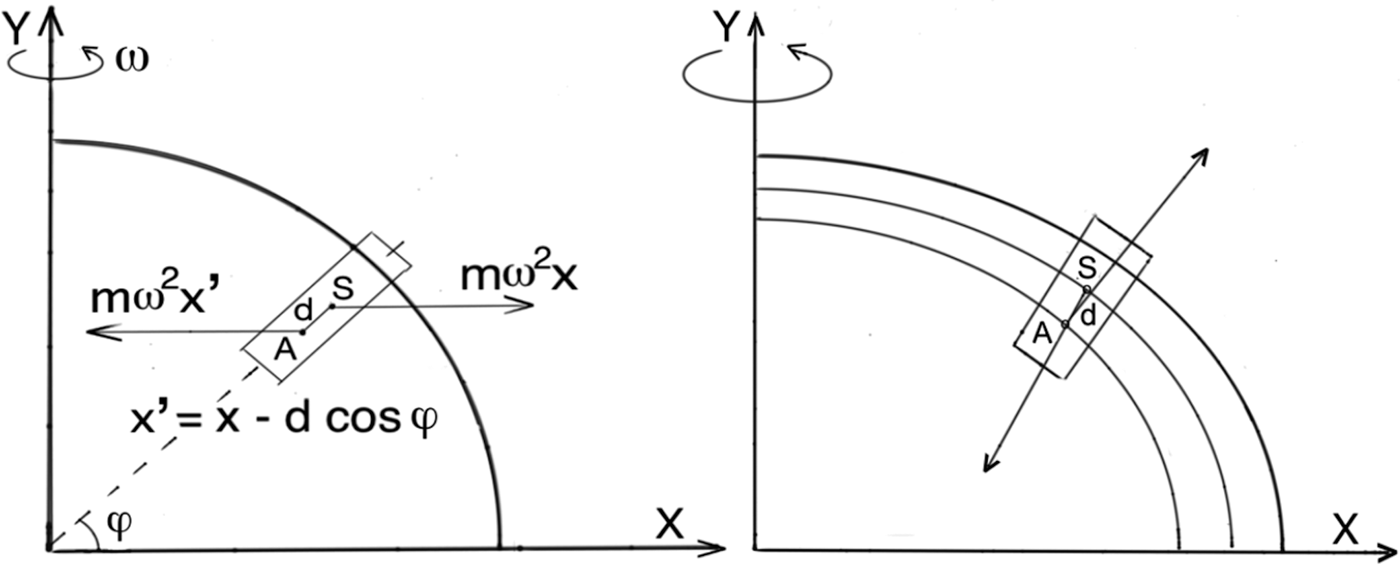
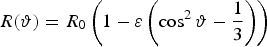
Fig. 1. Centrifugal and centripetal forces acting on the center of mass S and the center of buoyancy A, respectively. A and S are a distance d apart (left). Forces of gravity acting on the center of mass S and the center of buoyancy A are not exactly parallel owing to the oblateness of the Earth's geoid. Whereas the ocean surface is an equipotential surface, a surface raised a constant distance d above it is not, because the force of gravity is not constant on an oblate Earth. A residual horizontal force on the raised iceberg results (right).
This paper has the objective to derive the magnitude of the Polfluchtkraft. This force acts on ice shelves that can be considered as a source of gigantic potential icebergs only pinned at their periphery and at some sticky spots, and it influences the motion of icebergs. It provides a steady equatorward bias superimposed on all other forces influencing floating ice masses.
MAGNITUDE OF THE POLFLUCHTKRAFT
One can derive the Polfluchtkraft by considering the potential energy associated with an iceberg located at a given latitude compared with the situation where the water making up the iceberg is molten. This latter state defines potential energy zero. The excess in potential energy associated with the iceberg is obtained by starting in the molten state and raising each water molecule in the combined gravitational and centrifugal force field of the earth against the lines of force such as to build-up the iceberg (residual movements perpendicular to the lines of force do not further change the potential energy). By this procedure, one can obtain the excess potential in principle exactly from measurable quantities; namely, one needs to know the gravitational force exerted by the earth down to typical depths and up to typical heights reached by icebergs and can then evaluate the excess potential by taking the appropriate integral over the space filled by the iceberg.
For the purpose of the present treatment, the gravitational force will be modeled by a suitably accurate parametrization as described below. Before entering into the details, however, it should be noted that there are two independent small parameters in this problem:
-
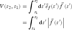
• The oblateness ε of the earth, defined by parametrizing the earth radius R as a function of latitude as
(1)i.e. as an expansion in Legendre polynomials, truncated at the quadrupole term. Latitude is measured in terms of the angle $$R(\vartheta ) = R_0 \left( {1 - {\rm \it \varepsilon} \left( {\mathop {\cos} \nolimits^2 \vartheta - \displaystyle{1 \over 3}} \right)} \right)$$
$\vartheta $
with
$\vartheta= 0$
at either the North or South Pole depending on the hemisphere under consideration. For the earth, ε ≈ 1/300.
$$R(\vartheta ) = R_0 \left( {1 - {\rm \it \varepsilon} \left( {\mathop {\cos} \nolimits^2 \vartheta - \displaystyle{1 \over 3}} \right)} \right)$$
$\vartheta $
with
$\vartheta= 0$
at either the North or South Pole depending on the hemisphere under consideration. For the earth, ε ≈ 1/300.
-
• The ratio δ = d/R 0, where d denotes the separation (along a line perpendicular to the ocean surface) between the center of mass of the iceberg and the center of mass of the displaced water (center of buoyancy) as shown in Fig. 1; R 0 is defined by the above parametrization of the earth radius.


The Polfluchtkraft will turn out to be an effect of order O(δε), and it is necessary to carefully keep all terms up to this order. Note that δ ≪ ε ≪ 1, i.e. one can neglect terms of order O(δ 2) with respect to terms of order O(δε).
Consider now successively building up the iceberg by raising water molecules against lines of the combined gravitational and centrifugal force
 $\vec f$
, as described above. The lines of force are characterized by the tangential unit vector
$\vec f$
, as described above. The lines of force are characterized by the tangential unit vector
 $\vec e_f = \vec f/\vert\vec f\vert$
, and if one transports a water molecule by an arc length s
2 − s
1, it acquires the potential energy
$\vec e_f = \vec f/\vert\vec f\vert$
, and if one transports a water molecule by an arc length s
2 − s
1, it acquires the potential energy
 $$\eqalign{ V(s_2, s_1 ) & = {\int}_{s_1} ^{s_2} {\rm d}s^{\prime}\vec e_f (s^{\prime})\vec f\,(s^{\prime}) \cr & = \int_{s_1} ^{s_2} {\rm d}s^{\prime}\left \vert {\vec f\,(s^{\prime})} \right \vert} $$
Expanding
 $\vert\vec f(s')\vert$
in a Taylor series in the arc length s′ around the point s′ = 0 where the line of force pierces the ocean surface, it is clear that the leading contribution to V is given by
$\vert\vec f(s')\vert$
in a Taylor series in the arc length s′ around the point s′ = 0 where the line of force pierces the ocean surface, it is clear that the leading contribution to V is given by
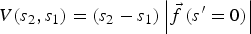 $$V(s_2, s_1 ) = (s_2 - s_1 )\left \vert {\vec f\,(s^{\prime} = 0)} \right \vert $$
because (s
2 − s
1) is of the order of d. Analogously expanding
 $\vec e_f (s')$
, the relation
$\vec e_f (s')$
, the relation
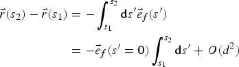 $$\eqalign{ \vec r(s_2 ) - \vec r(s_1 ) & = - \int_{s_1} ^{s_2} {\rm d}s^{\prime}\vec e_f (s^{\prime}) \cr & = - \vec e_f (s^{\prime} = 0)\int_{s_1} ^{s_2} {\rm d}s^{\prime} + O(d^2 )} $$
implies that, to leading order in d, the line of force can be regarded as straight and perpendicular to the ocean surface, and (s 2 − s 1) is nothing but the vertical displacement of the water molecule.
As a direct consequence, the excess potential energy of the entire iceberg at latitude
 $\vartheta $
can be calculated to leading order in d from the combined gravitational and centrifugal force (Fig. 1) at the ocean surface,
$\vartheta $
can be calculated to leading order in d from the combined gravitational and centrifugal force (Fig. 1) at the ocean surface,
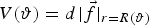 $$V(\vartheta ) = d{\kern 1pt} \vert \vec f \vert _{r = R(\vartheta )} $$
It should be noted that this argument strictly speaking is valid only for horizontal iceberg extensions of the order of d. However, icebergs can be orders of magnitude larger in the horizontal direction, such that the
 $\vartheta $
-dependence of
$\vartheta $
-dependence of
 $\vert\vec f\vert_{r = R(\vartheta )} $
should not be passed over without comment. Corrections due to this dependence are indeed suppressed by a factor of similar smallness as effects subleading in δ; namely, by a factor εγ, where γ denotes the ratio between the horizontal extension of the iceberg and the earth radius.
$\vert\vec f\vert_{r = R(\vartheta )} $
should not be passed over without comment. Corrections due to this dependence are indeed suppressed by a factor of similar smallness as effects subleading in δ; namely, by a factor εγ, where γ denotes the ratio between the horizontal extension of the iceberg and the earth radius.
To proceed, it is necessary to introduce a model for the gravitational and centrifugal force field at the ocean surface. This can be constructed as follows: Consistent with (1), the gravitational potential v G can be written as a rapidly converging expansion in Legendre polynomials, truncated at the quadrupole term,
 $$v_{\rm G} (r,\vartheta ) = v_0 (r) + {\it \varepsilon} v_2 (r)\left( {\mathop {\cos} \nolimits^2 \vartheta - \displaystyle{1 \over 3}} \right)$$
Also, this potential at (or, more precisely, anywhere above) the ocean surface must solve the Laplace equation Δv G = 0, which implies that
 $$v_{\rm G} (r,\vartheta ) = - GM\left( {\displaystyle{1 \over r} - \displaystyle{{{\varepsilon} B} \over {r^3}} \left( {\mathop {\cos} \nolimits^2 \vartheta - \displaystyle{1 \over 3}} \right)} \right)$$
with integration constants GM and B. Furthermore, in the rotating frame of reference of the earth, the iceberg experiences an centrifugal force, which can be described as originating from an additional effective potential
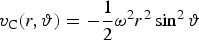 $$v_{\rm C} (r,\vartheta ) = - \displaystyle{1 \over 2}\omega ^2 r^2 \mathop {\sin} \nolimits^2 \vartheta $$
and the combined gravitational and centrifugal field of the earth is described by the sum v = v G + v C. Note that for the present discussion of the excess potential energy associated with an iceberg, the Coriolis force arising in the rotating frame of reference is irrelevant.
Before proceeding, it is useful to eliminate some of the diverse constants. On the one hand, the angular frequency ω in v C and the oblateness ε are related via the Earth's planetary dynamics. Empirically, for the Earth the relation
 $$\omega ^2 R_0^2 = {\it \varepsilon} \displaystyle{{GM} \over {R_0}} $$
is satisfied to a good approximation (Lang Reference Lang1980); note that if the earth were a homogeneous fluid ellipsoid, the right-hand side of this relation would appear multiplied by a factor 4/5. On the other hand,
 $R(\vartheta )$
represents an equipotential surface of v,
$R(\vartheta )$
represents an equipotential surface of v,
 $$0 = \displaystyle{{\rm d} \over {{\rm d}\vartheta}} v(R(\vartheta ),\vartheta ) = \left. {\displaystyle{{\partial v} \over {\partial \vartheta}}} \right \vert _{r = R(\vartheta )} + \left. {\displaystyle{{\partial v} \over {{\rm d}r}}} \right \vert _{r = R(\vartheta )} \displaystyle{{{\rm d}R} \over {{\rm d}\vartheta}} $$
whence, by solving with respect to
 ${\rm d}R/{\rm d}\vartheta $
and inserting the representations (1) and (7), (8) one obtains the relation
${\rm d}R/{\rm d}\vartheta $
and inserting the representations (1) and (7), (8) one obtains the relation
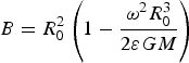 $$B = R_0^2 \left( {1 - \displaystyle{{\omega ^2 R_0^3} \over {2{\it \varepsilon} GM}}} \right)$$
to leading order in ε, where it should be observed, cf. (9) that ω 2 is a quantity of order O(ε).
Using (9) and (11) to eliminate the integration constants in v, one obtains
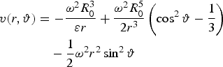 $$\eqalign{ v(r,\vartheta ) & = - \displaystyle{{\omega ^2 R_0^3} \over {{\rm \varepsilon} r}} + \displaystyle{{\omega ^2 R_0^5} \over {2r^3}} \left( {\mathop {\cos} \nolimits^2 \vartheta - \displaystyle{1 \over 3}} \right) \cr & \quad - \displaystyle{1 \over 2}\omega ^2 r^2 \mathop {\sin} \nolimits^2 \vartheta} $$
Consequently, the excess potential energy associated with an iceberg of mass m can be evaluated by inserting
 $\vert\vec f\vert = m\vert\vec \nabla v\vert$
into (5),
$\vert\vec f\vert = m\vert\vec \nabla v\vert$
into (5),
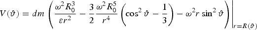 $$V(\vartheta ) = dm\left. {\left( {\displaystyle{{\omega ^2 R_0^3} \over {{\it \varepsilon} r^2}} - \displaystyle{3 \over 2}\displaystyle{{\omega ^2 R_0^5} \over {r^4}} \left( {\mathop {\cos} \nolimits^2 \vartheta - \displaystyle{1 \over 3}} \right) - \omega ^2 r\mathop {\sin} \nolimits^2 \vartheta} \right)} \right \vert _{r = R(\vartheta )} $$
 $$= dm\omega ^2 R_0 \left( {\displaystyle{1 \over {\it \varepsilon}} - \displaystyle{7 \over 6} + \displaystyle{3 \over 2}\mathop {\cos} \nolimits^2 \vartheta} \right)$$
to linear order in ε. Note that, to this order,
 $\vert\vec f\vert = m\partial v/\partial r$
. From this, the Polfluchtkraft F
p is simply given in terms of the gradient of V in the azimuthal direction. Specifically, a shift in latitude
$\vert\vec f\vert = m\partial v/\partial r$
. From this, the Polfluchtkraft F
p is simply given in terms of the gradient of V in the azimuthal direction. Specifically, a shift in latitude
 ${\rm d}\vartheta $
implies a change in potential
${\rm d}\vartheta $
implies a change in potential
 $${\rm d}V = \displaystyle{{{\rm d}V} \over {{\rm d}\vartheta}} {\rm d}\vartheta = - \displaystyle{3 \over 2}dm\omega ^2 R_0 \sin 2\vartheta {\kern 1pt} d\vartheta $$
whereas the distance induced by this shift is
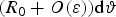 $(R_0 + O({\varepsilon} )){\rm d}\vartheta $
. Thus, one obtains for the Polfluchtkraft
$(R_0 + O({\varepsilon} )){\rm d}\vartheta $
. Thus, one obtains for the Polfluchtkraft
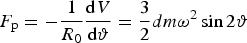 $$F_{\rm p} = - \displaystyle{1 \over {R_0}} \displaystyle{{{\rm d}V} \over {{\rm d}\vartheta}} = \displaystyle{3 \over 2}dm\omega ^2 \sin 2\vartheta $$
This result coincides with the one obtained by Epstein, seemingly by an accidental cancellation of errors, as discussed in the Appendix.
In terms of an operation on the model (7), (8) for the earth's combined gravitational and centrifugal potential, the Polfluchtkraft generally takes the form
 $$\eqalign{ F_{\rm p} & = - \displaystyle{1 \over {R_0}} \displaystyle{{\rm d} \over {{\rm d}\vartheta}} V(R(\vartheta ),\vartheta ) \cr & = - \displaystyle{1 \over {R_0}} \left. {\left( {\displaystyle{{\partial V} \over {\partial \vartheta}} + \displaystyle{{\partial V} \over {\partial r}}\displaystyle{{{\rm d}R} \over {{\rm d}\vartheta}}} \right)} \right \vert _{r = R(\vartheta )} = \displaystyle{{dm} \over {R_0 v_{\rm r}}} (v_{{\rm rr}} v_\vartheta - v_{{\rm r}\vartheta} v_{\rm r} )} $$
where the subscripts in the last expression denote partial derivatives. Here,
 $V = d\vert\vec f\vert = dmv_{\rm r} $
to linear order in ε was used, and
$V = d\vert\vec f\vert = dmv_{\rm r} $
to linear order in ε was used, and
 ${\rm d}R/{\rm d}\vartheta $
was expressed in terms of partial derivatives of v by using (10).
${\rm d}R/{\rm d}\vartheta $
was expressed in terms of partial derivatives of v by using (10).
MOVEMENT OF FLOATING ICEBERGS
How does a floating iceberg move under the influence of the Polfluchtkraft? If there were no friction of whatever kind, no Coriolis force and no ocean currents, the answer would be given in this ideal case of physics directly by the excess potential
 $V(\vartheta )$
and energy conservation.
$V(\vartheta )$
and energy conservation.
An iceberg starting at latitude
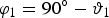 $\varphi _1 = 90{\rm ^\circ} - \vartheta _1 $
with its center of gravity on the potential surface effectively sinks to another surface with a potential difference of
$\varphi _1 = 90{\rm ^\circ} - \vartheta _1 $
with its center of gravity on the potential surface effectively sinks to another surface with a potential difference of
 $$\delta L = L^{\prime}_2 - L^{\prime}_1 = \displaystyle{3 \over 2}d\omega ^2 R(\mathop {\sin} \nolimits^2 \vartheta _2 - \mathop {\sin} \nolimits^2 \vartheta _1 )$$
while it reaches the latitude φ 2 and acquires the speed corresponding to this difference:
 $$v = \sqrt {3d\omega ^2 R(\mathop {\sin} \nolimits^2 \vartheta _2 - \mathop {\sin} \nolimits^2 \vartheta _1 )} $$
The potential (18) is formally identical to that of a mathematical pendulum (a mass suspended by a string of length l), which reads:
 $$L = - gl(1 - \cos \psi ) = - 2gl\mathop {\sin} \nolimits^2 \displaystyle{\psi \over 2}$$
One simply has to replace ψ/2 by φ and 2gl by (3/2)dω 2 R and omits the here irrelevant constant terms. Owing to this identity, the floating iceberg would oscillate around the equator exactly like the pendulum swings around the vertical plane. If and only if latitudes are low, the force is elastic, proportional to φ and the oscillation becomes sinusoidal:
 $$\varphi = \varphi _0 \sin \Omega t$$
Since
 $v = R\dot \varphi $
the oscillation angular frequency Ω and the oscillation period T in days become:
$v = R\dot \varphi $
the oscillation angular frequency Ω and the oscillation period T in days become:
 $$\Omega = \sqrt {\displaystyle{{3d\omega ^2} \over R}} ;\quad T = \sqrt {\displaystyle{R \over {3d}}} $$
For instance, with d = 100 m we obtain T = 112 days or 28 days for the trip from any low latitude to the equator. The speed is
 $$v = R\dot \varphi = \varphi _1 R\Omega \cos \Omega t$$
i.e. v = 2 m s−1 for φ 1 = 30° and d = 100 m.
This isochrony (independence of period on initial latitude) gets lost for higher latitudes, like with the pendulum for higher amplitudes. Then, the elementary expression for φ(t) must be replaced by elliptic integrals of the first kind. The speed can still be expressed as (19). Starting from 60° our iceberg with d = 100 m would attain the equator with a speed v = 3.5 m s−1 after 38 days.
The real movement of an iceberg is of course limited by frictional resistance in the ocean and by melting kinetics. As soon as a large iceberg breaks off from an iceshelf in Antarctica, it starts to move North under the influence of the Polfluchtkraft. It will reach a stationary speed v st when the Polfluchtkraft and the Newton resistance force F n in water are equal.
 $$F_{\rm p} = F_{\rm n} = \displaystyle{3 \over 2}dm\omega ^2 \sin 2\vartheta = \alpha A\rho v_{{\rm st}} ^2 $$
where α is a form factor, A is the frontal surface area, ρ is the density of water.
 $$v_{{\rm st}} = \sqrt {\displaystyle{3 \over 2}\displaystyle{{dm\omega ^2} \over {\alpha A\rho}} \sin 2\vartheta} $$
This stationary velocity oriented North gives rise to a Coriolis force F c oriented perpendicular to the West.
 $$F_{\rm c} = 2m\omega v_{{\rm st}} \cos \vartheta $$
This Coriolis force is ~10 times smaller than the Polfluchtkraft, and since the area A′ of an elongated iceberg moving sideways is ~10 times larger, the stationary velocity to the West is also ~10 times smaller. In addition, the general West to East moving circumpolar ocean current counteracts the Coriolis force. This is consistent with the generally observed dominance of movement to the North. Concentrating therefore on the equation of motion for the northward velocity, v,
 $$\dot v = - R\ddot \varphi = \displaystyle{3 \over 2}\omega ^2 d\sin 2\varphi - \displaystyle{{\alpha A\rho} \over m}R^2 \dot \varphi ^2 $$
can be integrated substituting φ with −φ and
 $$q(\varphi ) = \dot \varphi ^2 (t)$$
furnishing
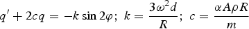 $$q^{\prime} + 2cq = - k\sin 2\varphi ;\;k = \displaystyle{{3\omega ^2 d} \over R};\;c = \displaystyle{{\alpha A\rho R} \over m}$$
This first order differential equation is solved by
 $$\eqalign{ q = &- \displaystyle{k \over {2c^2 + 2}}[c\sin 2\varphi - \cos 2\varphi - e^{2c(\varphi _0 - \varphi )} (c\sin 2\varphi _0 \cr &- \cos 2\varphi _0 )]}$$
and the velocity is
 $$v = R\sqrt q $$
which also respects the initial condition q = 0 for
 $\varphi = \varphi _{{\kern 1pt} 0} $
. We look for the turning point of the trajectory, where v = 0. Putting x = 2c
φ, it can be identified by the equation
$\varphi = \varphi _{{\kern 1pt} 0} $
. We look for the turning point of the trajectory, where v = 0. Putting x = 2c
φ, it can be identified by the equation
 $$f\,(x) = e^x \left( {\sin \displaystyle{x \over c} - \displaystyle{1 \over c}\cos \displaystyle{x \over c}} \right) = f\,(x_0 )$$
As a plot of this function shows, under consideration of
 $$c = \displaystyle{{\alpha \rho R} \over {\rho ^{\prime}l}}{\rm \gg} 1$$
Equation (32) is solved by x ≈ 1, i.e.
 $$\varphi _i = \displaystyle{1 \over {2c}};\quad R\varphi _i = \displaystyle{l \over 2\alpha} $$
The iceberg always shoots 1/α of its own length l beyond the equator.
It is also interesting to know, where the maximal speed occurs. Due to inertia, this is somewhat beyond the 45° parallel, where the force is at a maximum. The derivative of (30) vanishes at
 $$2e^x \left( {c\cos \displaystyle{x \over c} + \sin \displaystyle{x \over c}} \right) = 2c \left[{- e^{x_0} \left( {c\sin \displaystyle{{x_0} \over c} - \cos \displaystyle{{x_0} \over c}} \right)}\right]$$
This occurs at 35° for a typical iceberg of length l = 1000 km, at 43° for l = 100 km, at 44.4° for l = 10 km, and at 44.94° for l = 1 km.
The computation of the time for such a trip leads again to elliptic integrals. In the stationary case
 $$v_{{\rm st}} = R\sqrt {\displaystyle{k \over {2c}}\sin 2\varphi} = \sqrt {\displaystyle{3 \over 2}\displaystyle{{\omega ^2 dl} \over \alpha}\sin 2\varphi} $$
Calculating the Polfluchtkraft for real icebergs is impossible for lack of sufficient data. Instead, we present some results for a wide range of model icebergs in order to get some insight into the order of magnitude for this important force acting on floating ice masses. Figure 2 shows the quasi-stationary velocity of three icebergs, 1, 10 and 100 km long. The transit time from a starting position at latitude 65° is given in Fig. 3. If these icebergs are protected somehow from melting, they all reach the equator, the 1 km berg would theoretically get there in 18 years.
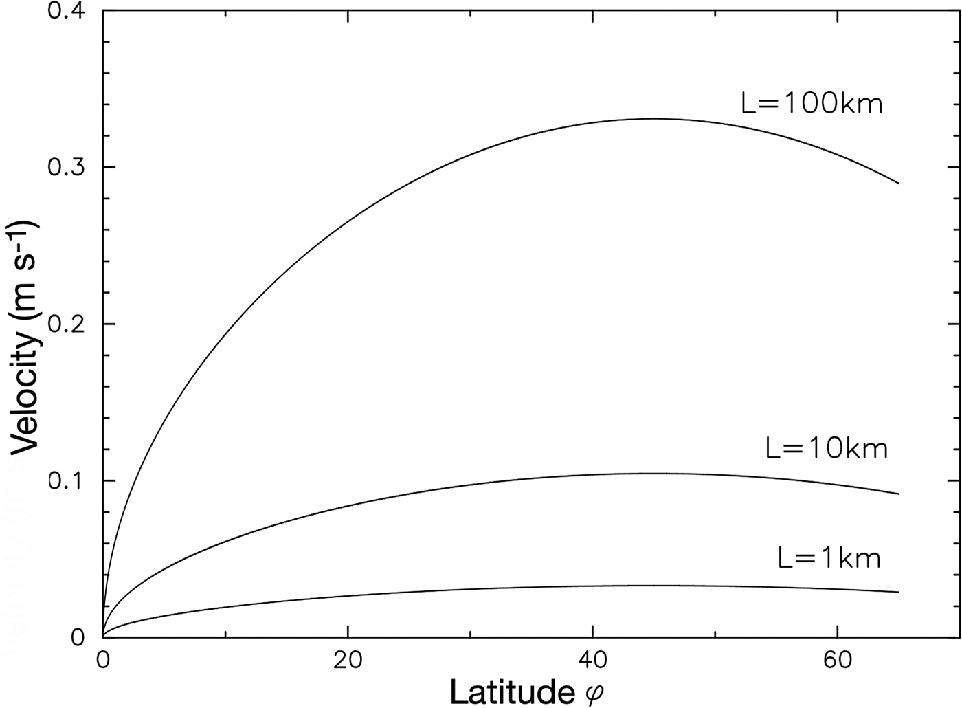
Fig. 2. Quasi-stationary velocity of icebergs 1, 10 and 100 km long and 300 m thick versus latitude starting at 65°S after reaching equilibrium between Polfluchtkraft and frictional force.
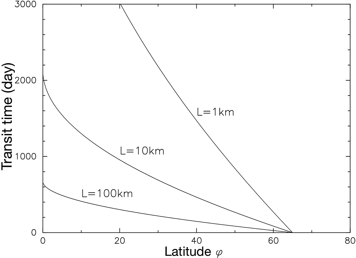
Fig. 3. Transit time of icebergs as in Fig. 2 starting at 65°S.
The relaxation time for obtaining the stationary speed is
 $$\tau = \displaystyle{{v_{{\rm st}}} \over {\dot v_{{\rm max}}}} = \sqrt {\displaystyle{2 \over {kc\sin 2\varphi}}} = \sqrt {\displaystyle{{2l} \over {3\alpha d\omega ^2\sin 2\varphi}}} $$
If the force would suddenly cease, within this time there would be an overshoot by a distance
 $$R\delta \varphi = R\dot \varphi \tau = R\displaystyle{1 \over c}$$
This is a good estimate for the overshoot beyond the equator as calculated above. Even in the stationary case, the time
 $$t = \int_{\varphi _1} ^{\varphi _2} \displaystyle{{{\rm d}\varphi} \over {\dot \varphi}} = \sqrt {\displaystyle{2c \over {k}}} \int_{\varphi _1} ^{\varphi _2} \displaystyle{{{\rm d}\varphi} \over {\sqrt {\sin 2\varphi}}} $$
cannot be expressed in elementary terms. Rather close to the equator, where φ ≪ 1
 $$t = \sqrt {\displaystyle{2c \over {k}}} \int_{\varphi _1}^{\varphi _2} \displaystyle{{{\rm d}\varphi } \over {\sqrt {2\varphi } }} = -2\left[{\displaystyle{R \over \omega }\sqrt {\displaystyle{\alpha \over {3ld}}} (\sqrt {\varphi _1} - \sqrt {\varphi _2} )}\right]$$
We have been discussing the trajectory of an iceberg whose mass and dimensions remain constant. Melting modifies this behavior by diminishing both the mass and the frontal surface of the iceberg. Melting is a complicated process, which can only be treated in a simplified manner. It greatly reduces the distances traveled by icebergs. Large icebergs often break-up into smaller pieces, which exposes them to more melting (Scambos and others, Reference Scambos, Sergienko, Sargent, MacAyeal and Fastook2005).
Without going into the details of such a modeling exercise, we find that, under plausible assumptions about the melting kinetics, icebergs released at 65° latitude with an initial thickness of 300 m and 100 km length as in Fig. 3 typically do not reach the equator, but only persist up to moderate latitudes.
Iceberg B-10, that originated as the floating tongue of Thwaites Glacier, broke off in 1992, ran aground for several years, was trapped and pushed in packice, and finally, in 1997, it escaped and started to travel North at an increasing speed helped by ocean currents and the Polfluchtkraft. The iceberg dimensions were 38 km × 78 km, the thickness is not well known. If all of its speed were due to the Polfluchtkraft, its thickness would have to be 1000 m. If only half of its speed were from Polfluchtkraft, its thickness would be 250 m. The fact that this iceberg survived such a long time indicates that it is very thick with the potential of traveling much further North. The importance of the Polfluchtkraft is also illustrated by a much smaller iceberg that broke off earlier from B-10. This iceberg was carried away by local ocean currents and wind towards the West, while the main iceberg B-10 took off in a northerly direction clearly assisted by the Polfluchtkraft against the prevailing ocean current.
INFLUENCE OF CURRENTS AND WINDS
Any ocean current carries of course the iceberg away with its speed
 $\vec w$
. The resultant speed is then the vector sum of
$\vec w$
. The resultant speed is then the vector sum of
 $\vec w$
and the equatorward speed due to the Polfluchtkraft and relative to the water, which we just estimated. The eastward currents driven by the West winds between 40° and 60°S have an average speed
$\vec w$
and the equatorward speed due to the Polfluchtkraft and relative to the water, which we just estimated. The eastward currents driven by the West winds between 40° and 60°S have an average speed
 $w \approx 0.2{\kern 1pt} \;{\rm m/s}$
, which is comparable with the Polflucht-drift speed of an iceberg ~100 km long. Such an iceberg ought to move in NE direction. The smaller an iceberg, the more eastward is its motion. The westward currents close to the Antarctic continent are somewhat faster. Moreover trapping in packice and stranding in shallow waters on the continental shelf can delay the progression of icebergs for several years.
$w \approx 0.2{\kern 1pt} \;{\rm m/s}$
, which is comparable with the Polflucht-drift speed of an iceberg ~100 km long. Such an iceberg ought to move in NE direction. The smaller an iceberg, the more eastward is its motion. The westward currents close to the Antarctic continent are somewhat faster. Moreover trapping in packice and stranding in shallow waters on the continental shelf can delay the progression of icebergs for several years.
The average wind velocity is some 20 times faster than the speed of ocean currents, but the wind hits only 1/7 as much surface as the current, and its density is 800 times lower. Thus, due to a force ρAv 2, the wind influences the course of an iceberg 5–10 times less than the ocean current. It is not uncommon to observe smaller icebergs and sea ice to move in one direction propelled by strong surface winds and larger icebergs moving in the opposite direction following mostly the combined ocean currents and the Polfluchtkraft.
ORIENTATION OF AN OBLONG ICEBERG
From the
 $sin2\vartheta $
-dependence follows that the Polfluchtkraft is largest at 45° latitude decreasing towards the equator and the pole. An oblong iceberg experiences a torque that tends to align the berg in N–S direction when traveling between the pole and 45° and in E–W direction traveling from there to the equator.
$sin2\vartheta $
-dependence follows that the Polfluchtkraft is largest at 45° latitude decreasing towards the equator and the pole. An oblong iceberg experiences a torque that tends to align the berg in N–S direction when traveling between the pole and 45° and in E–W direction traveling from there to the equator.
How long would it take to rotate an iceberg into its equilibrium position? The torque is
 $$D = L^2 \displaystyle{{{\rm d}F_{\rm p}} \over {R{\rm d}\varphi}} \approx \displaystyle{{3L^2 md\omega ^2 cos2\varphi} \over R} \approx \displaystyle{{3L^3 WH^2\Delta \rho \omega ^2 cos2\varphi} \over R}$$
L, W, H is the length, width and height of the iceberg, Δρ is the difference of water and ice densities.
The opposing torque from friction in water is of the order
 $$D_{\rm r} = L^2 Hv^2 \rho = L^4 H\omega^{\prime 2} \rho $$
where ω′ is the angular velocity of rotation of the iceberg. The result is
 $$\omega ^{\prime} \approx \sqrt {\displaystyle{{WH\Delta \rho} \over {RL\rho}}} \omega $$
With W = H = 1 km and L = 10 km the rotation about an angle of order 1 rad would require ~2 years. It is observed that large tabular icebergs do not rotate much unless they break-up, melt, get grounded, or collide with other obstacles. But if the iceberg lingers around at high latitudes for long enough time it might be able to gain an orientation most favorable for traveling North. This is indeed true for iceberg B-10. At latitude 60° South its long axis was oriented exactly N–S.
CONCLUSIONS
We have reformulated an important force acting on icebergs. The Polfluchtkraft was originally recognized by several geophysicists including Alfred Wegener. It forces large icebergs to move toward the equator. The velocities of large icebergs propelled by this force are comparable with or exceeding the velocities of ocean currents. Thickness is of particular importance. If an iceberg could be protected from melting or breaking up into pieces, it could easily reach lower latitudes and be used as a source of fresh water.
Most importantly, ice shelves, like the Ross Ice Shelf and the Ronne Ice Shelf, are gigantic floating ice masses, which are also subject to the Polfluchtkraft. As global warming weakens their attachment to peripheral shear margins and to pinning points and as it is filling crevasses with meltwater, the Polfluchtkraft could be the final straw for their demise. Consequently, the ice streams feeding the ice shelves will lose the backpressure from the ice shelves. They will speed up, accelerating the decay of the whole ice sheet and contributing to rapid sea-level rise (Rignot and others, Reference Rignot2004; Scambos and others, Reference Scambos, Bohlander, Shuman and Skvarca2004; Joughin and Alley, Reference Joughin and Alley2011; Joughin and others, Reference Joughin, Smith and Medley2014).
During ice-sheet surges or ice-shelf disintegration, huge armadas of icebergs are propelled towards the equator, interrupting ocean temperatures and possibly changing ocean circulation, which could lead to additional abrupt climatic changes. This seems to have happened during Heinrich events (Broecker, Reference Broecker1994; Hulbe and others, Reference Hulbe, MacAyeal, Denton, Kleman and Lowell2004).
The present disintegration of the Larsen Ice Shelf and the discharge of Pine Island Glacier, Thwaites Glacier and several large Antarctic icebergs in recent years are not just isolated episodes, but precursors of a bigger event, the disintegration of the West Antarctic ice sheet resulting in rapid sea-level rise of several meters. The Polfluchtkraft is standing by for the Big Move.
ACKNOWLEDGEMENTs
We thank several reviewers and the Editor for constructive suggestions. The late Helmut Vogel, a superb experimental physicist inspired us in his famous physics class by performing the classic Lely experiment that demonstrated the force acting on an object floating on a rotating liquid.
APPENDIX - EPSTEIN'S PROCEDURE
Epstein constructs a Lagrangian potential function for the combined gravitational and centrifugal field in the reference frame of a planet rotating with angular frequency ω, obtaining
 $$L = \displaystyle{1 \over 2}\omega ^2 r^2 \mathop {\sin} \nolimits^2 \vartheta + \displaystyle{{GM} \over r} - \displaystyle{C \over r}\mathop {\sin} \nolimits^2 \vartheta $$
Here,
 $\vartheta $
counts as usual from the North Pole, whereas Epstein uses the geographical latitude. From this
$\vartheta $
counts as usual from the North Pole, whereas Epstein uses the geographical latitude. From this
 $L(r,\vartheta )$
, he constructs the force on an object of mass m perpendicular to the radius vector:
$L(r,\vartheta )$
, he constructs the force on an object of mass m perpendicular to the radius vector:
 $$F_\vartheta = m\displaystyle{1 \over r}\displaystyle{{\partial L} \over {\partial \vartheta}} = m\left( {\displaystyle{1 \over 2}\omega ^2 r - \displaystyle{C \over {r^2}}} \right){\kern 1pt} \sin 2\vartheta $$
He determines C for the surface of the planet from the fact that this force has to vanish, i.e.
 $$C = \displaystyle{1 \over 2}{\kern 1pt} \omega ^2 R^3 $$
Epstein then forms the Lagrangian at a distance r + d instead of r from the center, i.e. at the center of gravity of the floating body instead of its center of buoyancy. The
 $\vartheta $
-dependent part of this Lagrangian is
$\vartheta $
-dependent part of this Lagrangian is
 $$\left( {\displaystyle{1 \over 2}\omega ^2 (r + d)^2 - \displaystyle{C \over {r + d}}} \right)\mathop {\sin} \nolimits^2 \vartheta $$
He derives the corresponding force
 $F'_\vartheta = F_\vartheta (r + d)$
, which, to linear order in d, i.e. close to the surface r = R, reads
$F'_\vartheta = F_\vartheta (r + d)$
, which, to linear order in d, i.e. close to the surface r = R, reads
 $$F^{\prime}_\vartheta = F_\vartheta + \displaystyle{3 \over 2}md\omega ^2 {\kern 1pt} \sin 2\vartheta $$
where (46) was used. The difference
 $$F_{\rm p} = \displaystyle{3 \over 2}md\omega ^2 \sin 2\vartheta $$
is interpreted as an equatorward force acting on a floating object, since the displaced liquid was at an equilibrium, and hence
 $F_\vartheta = 0$
.
$F_\vartheta = 0$
.
The whole procedure could be applied to any Lagrangian
 $L(r,\vartheta )$
, and amounts to identifying
$L(r,\vartheta )$
, and amounts to identifying
 $$F_{\rm p} = m\displaystyle{d \over r}L_{r\vartheta} $$
where the subscripts mean partial derivatives, which should be contrasted with the correct expression (17). The difference between the two expressions stems from the fact that Epstein assumes the vector by which the center of mass of the floating body differs from the center of buoyancy to be proportional to a radial vector viewed from the center of the earth, as described after Eqn (46). While this constitutes a good approximation for many applications, the error is precisely of linear order in ε, i.e. the order which is relevant for the Polfluchtkraft. Instead, the floating body is raised by a vector perpendicular to an equipotential surface of the combined gravitational and centrifugal field, such as the ocean surface. In the same way, Epstein also neglects in his determination of the constant C the fact that the ocean surface is not quite perpendicular to a radial vector; he determines C from the requirement
 $\partial L/\partial \vartheta = 0$
, instead of using a self-consistent condition such as (10). The errors are of linear order in ε and thus quite essential.
$\partial L/\partial \vartheta = 0$
, instead of using a self-consistent condition such as (10). The errors are of linear order in ε and thus quite essential.
Nevertheless, Epstein obtains the correct magnitude of the Polfluchtkraft, Eqn (49). This hinges crucially on his ansatz (44), which in turn is questionable, since the gravitational part does not obey the Laplace equation. If Epstein had assumed a different power of r in the last term of (44), cf. the more realistic ansatz (7), he would have arrived at a Polfluchtkraft different from (49). Thus, Epstein's correct result (49) is seemingly due to a fortuitous cancellation of errors.
Applied to the correct potential (7), Epstein's procedure as described above leads to the identification
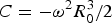
 $GM{\rm \epsilon} B = - \omega ^2 R_0^5 /2$
in analogy to (46), i.e. to the wrong sign of B, cf. (9) and (11). Further inserting into (50), one obtains
$GM{\rm \epsilon} B = - \omega ^2 R_0^5 /2$
in analogy to (46), i.e. to the wrong sign of B, cf. (9) and (11). Further inserting into (50), one obtains
 $$F_{\rm p} = m\displaystyle{d \over r}L_{r\vartheta} = \displaystyle{5 \over 2}md\omega ^2 {\kern 1pt} \sin 2\vartheta $$
which is of the wrong magnitude. If one instead correctly identifies
 $GM{\rm \varepsilon} B = \omega ^2 R_0^5 /2$
, cf. (9) and (11), then application of Epstein's prescription (50) yields
$GM{\rm \varepsilon} B = \omega ^2 R_0^5 /2$
, cf. (9) and (11), then application of Epstein's prescription (50) yields
 $$F_{\rm p} = m\displaystyle{d \over r}L_{r\vartheta} = - \displaystyle{1 \over 2}md\omega ^2 {\kern 1pt} \sin 2\vartheta $$
i.e. a force in the wrong direction, namely poleward.
Conversely, the correct procedure applied to Epstein's potential leads to the identification
 $C = - \omega ^2 R_0^3 /2$
in analogy to (11), i.e. the reverse sign as compared with (46). Then, inserting into (17), one obtains
$C = - \omega ^2 R_0^3 /2$
in analogy to (11), i.e. the reverse sign as compared with (46). Then, inserting into (17), one obtains
 $$F_{\rm p} = - \displaystyle{{md} \over {R_0 L_r}} (L_{rr} L_\vartheta - L_{r\vartheta} L_r ) = \displaystyle{5 \over 2}md\omega ^2 \sin 2\vartheta $$
i.e. the wrong magnitude. On the other hand, if one uses Epstein's identification C = ω 2 R 3/2, then application of (17) yields the correct result
 $$F_{\rm p} = - \displaystyle{{md} \over {R_0 L_r}} (L_{rr} L_\vartheta - L_{r\vartheta} L_r ) = \displaystyle{3 \over 2}md\omega ^2 \sin 2\vartheta $$
just as when using Epstein's procedure. This is not surprising, because if one determines C such that
 $L_\vartheta $
vanishes, as Epstein does, then (17) and (50) are equal.
$L_\vartheta $
vanishes, as Epstein does, then (17) and (50) are equal.


 Open access