


Introduction
Like many other glaciers in France, Glacier Blanc first attracted interest during the Little Ice Age in the seventeenth century, when its advance destroyed the Prė de Madame Carle. This field was a prairie used as a grazing area. Now, after 30 years of intense retreat, the 1978–85 advance renews interest in this glacier because the footbridge on the trail leading to the refuge du Glacier Blanc is threatened. Because part of this trail is already covered by ice, the Parc des Ecrins has requested a forecast of probable glacial activity for the coming 10 years.
In the following study we first present the measurements of variation in length that have been made on Glacier Blanc, and then use these data to attempt to answer the questions posed by Parc des Ecrins. Two different methods are used: one based on a statistical model, the other on a numerical model.
Review of Measurements Taken
Glacier Blanc, located in the National Parc des Ecrins, extends from the summit of the Ecrins at 4102 m a.s.l. down to 2300 m over a distance of 6 km and has a surface area of 7.7 km2 (Fig. 1). Its name comes from its very clean surface which, with very little rock debris, contrasts strongly with that of its neighbour, Glacier Noir, which is covered by about 300 mm of rock debris on the ablation tongue.
The oldest document relating to Glacier Blanc that has been found describes its seventeenth century advance and the destruction of the Pré de Madame Carle (Reference MouginMougin, 1930). At that time Glacier Blanc formed a common ablation tongue with Glacier Noir, although there is no indicator that allows the position of the front to be determined at that time. The first data are found around 1815, when the two glaciers reached the Cezanne mountain hut. This was the greatest advance in the last century and marked the end of the Little Ice Age in this area. Since 1870 the more-or-less regular survey of glaciers in the Alps makes it possible to describe the history of their variation in length. After the last maximum of the Little Ice Age there was a strong retreat, interrupted by minor advances in the 1890s, 1920s, and the one presently observed. The retreat of the 1940s is noteworthy because of its magnitude; it has greatly modified the glacial landscape of the Alps.

Fig. 1. Aerial photograph of Glacier Blanc in 1980, with the past locations of the front in 1904, 1890, 1880 and the two measurement profiles on the glacier tongue. Copyright IGB Paris, by authorization No. 522/IGN/Lyon.
In 1921, Pierre Mougin, Eaux et Forêts, initiated a programme of more regular and precise measurements of Glacier Blanc (Table I; Fig. 2). The contours of the glacier front were mapped, and elevation and velocity measurements were made for two fixed profiles across the ablation zone. The programme continued until 1966 and in 1975 a map of the ablation zone was produced. Since 1980 the programme of Eaux et Forêts has been taken over by the LGGE.
The Recent Problem
Table I. Distance between the front of glacier blanc and the lower profile (fig. 1). 1921–66 and 1975: eaux et forets. 1978: ign. 1971, 1972, 1980–87: lgge

Glacier Blanc is very popular with tourists and has easy access by a well-maintained footpath. Until 1980 the path leading to the Glacier Blanc hut ran along a ledge in the rock face of the left bank of the glacier. However, the 1978–85 advance of the glacier made this path very difficult to use. In order to restore easy access to the hut, it would be necessary to make a new path and also to build a new footbridge across the glacier stream, which would involve substantial cost to the Pare. For this reason, the Pare needed an estimate of the predicted movements of the glacier front in the following 10 years.
The necessary study was made using two contrasting methods. The first of these is purely statistical, and establishes a relationship between variations in length and in mass balance of the glacier. The second is based on a model of the ice-flow mechanics of the glacier as a whole. These methods have been used in other similar forecast studies; the first method was used byReference Graard Graard (1971) on Glacier d’Argentière; the second method was used by Reference NyeUntersteiner and Nye (1968) for Berendon Glacier in Canada which was threatening the access to a mine, and byReference Bindschadler Bindschadler (1980) for Griesgletscher in Switzerland, which is calving into an artificial lake. The predictions obtained by use of these methods did not produce a very accurate description of the front variations, especially when a maximum or a minimum was observed.
Forecast Using The Statistical Method
The annual variation in length of a glacier is the result of a complex interaction between the distribution of its mass balance and the shape of the glacial valley. Since it is difficult to quantify all the effects which are operating, we relate the variations in glacier length with the mass balance through a simple linear relationship:
where Δl(t) is the variation of length measured for year t, b(t − i) is the mass balance for year t = i, and a, a 0, a 0, a 1, … ai are coefficients determined by the least-squares method.
Because mass-balance measurements on Glacier Blanc were started only in 1979, we have also made use of available measurements for Sarenne Glacier, which were first recorded in 1949 (Fig. 6) and which have been reconstructed from 1882, using a statistical correlation with summer temperatures, June precipitations, and winter precipitations, by Reference MartinMartin (1978). It is possible to do this because it has been shown that a strong homogeneity of mass-balance variations exists within a mountain range (Reference ReynaudReynaud, 1980).

Fig. 2. Computed length of Glacier Blanc using the numerical method, compared with actual measurements. Equilibrium lengths reached for the different cases tried are shown on the right side of the plot. (For b = −1.34 m, the value is 5100 m.)

Fig. 3. Correlation coefficients between Glacier Blanc length variations and Sarenne Glacier mass balance at successive lag points (years).
For the length measurements, we have limited the period of definition of ai coefficients to the years 1960–85 because this is the only period for which the front had the same morphology as it now has (earlier, when the glacier was longer, it ended in a serac fall.)
To find out which mass-balance time lags are important, simple correlation coefficients between the Δl(t) series and b(t − i) have been computed and plotted in Figure 3. It appears that the correlations are significant at the 5% level only for lags of 13–19 years. The front of the glacier seems to react to change in mass balance with a time delay of about 15 years, and this delay spreads over 5 years. To model this effect, a multiple correlation is better than a simple correlation. The multiple correlation coefficient reaches 0.86 for mass balances with lags of 13, 14, 15, and 18 years. The corresponding regression equation is:

The accumulated Δl(t) values yield a picture of the evolution of the length of the glacier. The resulting curves using both measured and estimated l(t) values are plotted in Figure 4. The estimated curve does not reproduce the measured curve exactly, but it is quite close to the general trend. With the regression equation, it is possible to estimate

Fig. 4. Reconstructed and measured length variations of Glacier Blanc, and forecasts derived from the statistical method.
the variations of the front for the next 13 years without making any assumptions about mass balance. Error bars based on the standard error observed for the regression period have been plotted. It is obvious from the plot that for dates after 1990 the magnitude of error is very large, and that for this period the forecast has a diminished value. However, one possibility that seems unlikely actually to occur is a very rapid retreat of the glacier. The values for the glacier for the years 1986 and 1987, which were known and added after the prediction was made, provide a test of the method. These values correspond to the maxima of the error limit. It is also possible to compute values for the front before 1959 and to compare them with the measurements obtained. The predictions for the 4 years before the regression period (1955−58) show good agreement with the real measurements. The estimates for the years before 1955 are not very satisfactory, but this may be due to the changed morphology of the glacier front.
Forecast With The Numerical Model
The dynamics of the glacier are simulated with a one-dimensional ice-flow model, similar to that which Bindschadler (1980) andReference Oerlemans Oerlemans (1986)have used. Only plane shearing flow is considered. This model can be formulated in terms of a diffusion equation with a nonlinear diffusion coefficient, D(x), such that


where H is the thickness of ice, h is the elevation of the surface, x is the distance along a flow line, ρ is the density of ice, g is the acceleration due to gravity, b is the surface mass balance, and A and n are the flow parameters of Glen’s flow law (n is taken as equal to 3).
The following data are required as input to the model:
Bedrock profile.
Mass-balance distribution along the glacier.
Time evolution of this distribution (forcing function).
The model output gives the ice thickness and length variations with time.
The bedrock profile of Glacier Blanc is known only in parts near the glacier front, where drillings were made byReference Benoit Benoît (unpublished), and under the accumulation basin, where seismic measurements were made by Reference GluckGluck (1969). The missing sections are deduced from the surface profile. Figure 5 shows the bedrock profile that was used in this study and also the surface profile along the central flow lines of the glacier. A parabolic distribution of the mass balance was used, where b = 4 × 10⁻⁶(z − e) (z − e − 2000). It gives the simplest realistic curve to fit the values observed on the glacier, which are 8 m of ablation at the glacier front, and 0 m at the Glacier Blanc equilibrium line (e), at an altitude of around 3000 m. Accumulation depth is not known, and 4 m was estimated as the maximum likely value.
For the time evolution of this distribution we used the Sarenne Glacier mass-balance series (Fig. 6). A linear relationship between the mass balance, b(t), and the equilibrium-line altitude of Glacier Blanc, e(t), was assumed to be
where ![]() the mean mass balance of Sarenne Glacier for the 1882–95 period, and d(e)/db = 1/0.006, where 0.006 is the balance gradient which we have derived from a study of western Alpine glaciers.
the mean mass balance of Sarenne Glacier for the 1882–95 period, and d(e)/db = 1/0.006, where 0.006 is the balance gradient which we have derived from a study of western Alpine glaciers.
The flow-law constant 2A/5 in Equation (4) was computed for typical values for the accumulation basin. For a mean slope 0.1, a thickness H = 300 m, and a velocity 50 m a−1, the basal shear stress has a value of
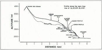
Fig. 5. Glacier Blanc profile along the central flow line. The 1904 surface elevation is taken from the Jacob and Flusin map (1905), the 1967 surface elevation from the IGN map.
2.7 × 10⁵ kg m−1 s−2 and the constant 2A/5 is equal to 8 × 10⁻¹⁸. Spatial differentials have been approximated by centred finite differences, and temporal differentials by forward differences. The grid spacing applied is 200 m, and the time step is 0.1 a. In order to obtain a more detailed description of front movements than can be obtained with the 200 m grid spacing, a corrective term, C, based on a linear extrapolation from the ice thickness, H i, of the last point was added, giving

where H m is the maximum thickness value for the last grid point for the glacier.

Fig. 6. Glacier mass-balance series used in the numerical model. Values for the period 1948–85 were measured (Valla, unpublished data). The other values were reconstructed by Martin (1978). The centred cumulative representation was chosen because the major events appear more clearly. The mean and the standard deviation of the whole series are respectively −0.48 and 0.87 m.
The initial condition of the glacier in 1882 was constructed on bare bedrock over 600 years of simulated time using a constant value correponding to the mass balance averaged for the period 1882–87. The sequence of e variations derived from the Sarenne Glacier mass balance was then applied. The exact e value for Equation (5), which is not known, was adjusted to 2995 m, so that the values for the final part of the curve approximately correspond to the observed glacier length. The resulting series of glacier lengths is plotted in Figure 6. Computation was continued beyond 1985 until equilibrium was reached for the following constant values for mass balance:
0.4 m, −1.34 m (mean for 1882–1985 plus or minus the standard deviation),
−0.3 m, −0.64 m (maximum and minimum of the 95% confidence interval),
−0.48 (mean).
The first two cases correspond to extreme situations, and show that even if a very negative sequence of mass-balance values occurred, the glacier would not start appreciably to retreat until at least 1990. All other hypotheses predict an increase in the length of the glacier. It takes anything from 15 to 80 years for equilibrium to be reached, and the predicted position of the glacier differs by as much as 2 km from one hypothesis to another. This shows two things: first, that the glacier is very sensitive to variations in mass balance, and secondly (because reaction times are at least a few years even for a small change in the mass balance) that the glacier is not very often in equilibrium.
Discussion of The Two Models
The numerical model is a very simplified one-dimensional model. Details of the nature of the bedrock of the glacier are not very well known. The computed velocities of the ice do not give a good match with reality (they reach only 30–50% of the observations). However, variations in length are rather well simulated. In order to obtain realistic variations of length with this type of model, it is very important to introduce a reliable mass-balance (or e) series. The results seem to depend more on the climatic series which is used than on the nature of the model itself. The advantage of the numerical model for forecasting is that it is still valid when the glacier undergoes large changes, and it can therefore describe variations over a longer time span than is possible with the statistical model. Furthermore, it describes the evolution of the whole glacier, not just of the glacier front. However, it requires more glacier data (bedrock and surface mapping), and the shape of the glacier must also be simple enough to be simulated by a one-dimensional model.
The statistical model is simpler to use and less data are necessary for its operation. It requires only measurements of length variations in the glacier and a mass-balance series for a glacier from the same mountain range. What is more, the short-term forecasts obtained using it are more detailed.
Conclusion
In order to forecast with the numerical model described, it is necessary to make assumptions about the mass balance of a glacier, and different cases have been tried. Only the most negative case (mean negative standard deviation) produces a retreat of the glacier front after a stable period of 5 years. Such a situation over a whole decade is an extreme that has been observed only during the 1940s. When the limits of the 95% confidence interval of the 1882–1985 mass-balance series are used, the model forecasts a slow advance of the front. This corresponds to the recovery of the glacier due to the above-average mass balance values for the past 20 years, which contrast with the previous low mass-balance values.
To forecast with the statistical model, no mass-balance assumptions are necessary. The results from such a model predict a 20–30 m retreat of Glacier Blanc until 1990, followed by a period of advance of the glacier.
The forecasts of the two models are different, but for the 1985–90 period, neither of the models suggests that a retreat of more than 20 m is probable. According to the numerical model, the footbridge could be destroyed as soon as 1985. For the 1985–90 decade, the statistical model suggests that the glacier will get very close to the footbridge, but will not destroy it. In any case, in 1986, since it seems unlikely that the glacier would retreat rapidly enough to clear the old path, the Pare has built a new path. This new path, farther away from the glacier, no longer uses the footbridge.


