


Introduction
Scientific studies using remote-sensing data in the past were primarily focused on land-use classification and long-term temporal changes in terrestrial land cover, assuming flat terrain in order to avoid complexities due to topography (Reference SandmeierSandmeier 1995). The strong variations in topographical parameters (mainly slope, aspect and altitude) in rugged mountainous terrain significantly influence the qualitative and quantitative analysis of snow cover (Reference Dozier and MarksDozier and Marks, 1987). The relief effect due to topography is neither eliminated during system correction nor during the normal geometric correction and has great significance in mountainous regions. Therefore, the impact of topography must be carefully examined prior to interpretation of remote-sensing data for snow-cover applications.
Various topographic correction methods are reported in the literature (Reference Riaño, Chuvieco, Salas and AguadoRiaño and others, 2003; Reference Nichol, Hang and SingNichol and others, 2006), including cosine-law method, C-correction, Minnaert corrections and slope matching. However, these have not been explored very extensively for snow-cover applications in Himalayan terrain. Most research is focused exclusively on vegetation analysis (Reference Riaño, Chuvieco, Salas and AguadoRiaño and others, 2003; Reference Nichol, Hang and SingNichol and others, 2006).
In this study, we carry out an extensive comparative performance analysis of different topographic normalization methods for snow-cover applications in rugged Himalayan terrain using Advanced Wide Field Sensor (AWiFS) and Moderate Resolution Imaging Spectroradiometer (MODIS) satellite data. The main objectives in the present paper are (1) qualitative performance analysis, (2) quantitative analysis of snow reflectance after topographic corrections, (3) validation of the spectral reflectance with in situ observations and (4) graphical analysis. Image-based atmospheric correction (Reference ChavezChavez, 1989; Reference Song, Woodcock, Seto, Lenney and MacomberSong and others, 2001) for path radiance and Rayleigh scattering is performed first for initial estimation of spectral reflectance without considering topographic influences. The details of implementation of these corrections on satellite imageries are reported by Reference Mishra, Negi, Rawat, Chaturvedi and SinghMishra and others (2009).
Topographic Models: A Brief Review
Image-based atmospherically corrected target spectral reflectance on the tilted surface, R AT, from sensor radiance, Lλ , is obtained using the following model (Reference Pandya, Singh, Murali, Babu, Kirankumar and DadhwalPandya and others, 2002; Reference Shepherd and DymondShepherd and Dymond, 2003):
where Lp is the path radiance in mW cm−2sr−1 μm−1 and estimated according to Reference Moran, Jackson, Slater and TeilletMoran and others (1992), and d is the Earth-Sun distance in astronomical units and calculated using the approach of Reference Van der MeerVan der Meer (1996). E 0 is bandpass exoatmospheric spectral irradiance (Tables 1 and 2), Ed is downwelling spectral irradiance at the surface due to diffused radiation and assumed equal to zero according to Reference ChavezChavez (1989), θ z is the solar zenith angle and calculated (Reference KastenKasten, 1962) for each pixel of the study area, tv is atmospheric transmittance along the path from ground surface to sensor and tz is atmospheric transmittance along the path from Sun to ground (Table 3) and calculated for the AWiFS and MODIS spectral bands using the model (Reference Pandya, Singh, Murali, Babu, Kirankumar and DadhwalPandya and others, 2002). The parameter Et is the terrain irradiance contributed due to reflected radiation from the adjacent terrain. The effect needs to be included in topographic correction for satellite data with fine spatial resolution (Reference Liu, Noumi and YamaguchiLiu and others, 2009). In case of coarse spatial resolution, it is negligible (Reference RichterRichter, 1998), so it is not considered in the present work for AWiFS and MODIS satellite data.
Table 1. Salient specifications of AWiFS sensor
Table 2. Salient specifications of MODIS sensor
Table 3. Atmospheric transmissivity in different spectral bands of AWiFS and MODIS
Cosine law
Cosine law is the most commonly used method and is based on a trigonometric approach assuming the surface to be Lambertian. The spectral reflectance is computed as (Reference Teillet, Guindon and GoodenoughTeillet and others, 1982)
where R λH is spectral reflectance for a horizontal surface, R λT is spectral reflectance observed over inclined terrain and cosi is illumination (IL) and calculated using the equation proposed by Reference CivcoCivco (1989).
C-correction
C-correction is based on the assumption of a non-Lambertian surface and is a modification of cosine correction developed by Reference Teillet, Guindon and GoodenoughTeillet and others (1982). A quantity, cλ, is introduced into Equation (2) defined as:
where cλ = (bλ/mλ ) is a quotient between intercept (bλ ) and slope (mλ ) in different spectral bands. It is estimated using a regression equation assuming the linear relationship between original uncorrected reflectance and cos i as:
Minnaert methods
Minnaert methods are non-Lambertian and based on the ideas of Reference MinnaertMinnaert (1941) who first proposed a semi-empirical equation to assess the roughness of the Moon surface. The function has been used for photometric analysis of lunar surfaces (Reference Holben and JusticeHolben and Justice, 1980) and implemented for topographic corrections as follows:
where k(λ) is the Minnaert constant and depends on the type of surface and spectral wavelength bands. It varies from 0 (ideally non-Lambertian surface) to 1 (perfect Lambertian surface). Equation (4) was further modified by Reference ColbyColby (1991) to include terrain slope, θp, as follows:
The value of k(λ) can be determined by linearizing Equation (5).
Slope-matching method
The slope-matching method was proposed by Reference Nichol, Hang and SingNichol and others (2006) who introduced certain modifications to Reference CivcoCivco’s (1989) model and considered the topographic corrections in two stages. They observed that Reference CivcoCivco’s (1989) topographic corrections do not improve the results in shady areas. In order to enhance the results on the north-facing slopes in the shadow area, equalization of radiance is required with respect to Sun-facing slopes to make the extent of corrections equal to the maximum difference of radiance values on both aspects. The final reflectance for topographic correction by Reference Nichol, Hang and SingNichol and others (2006) is estimated using:
where R nλij is the normalized reflectance values for image pixel ij in waveband λ, Rλ ij = RλT is the uncorrected original reflectance on the tilted surface for image pixel ij in waveband A, Rmax and R min are the maximum and minimum reflectance values, 〈cos i〉s is the scaled (0–255) mean IL on the south aspect and Cx is the coefficient estimated for each AWiFS and MODIS spectral band using the equation proposed by Reference Nichol, Hang and SingNichol and others (2006). The slope-matching method adjusts the brightness between northern and southern slopes. As such, its parameters depend on the image itself. It may perform very well for in-image adjustments, but its results may not be comparable between different images, as each image has its own statistics.
Methodology
Study area
Three study areas are considered in the present work. The first is located at 34.6124–34.7593° N, 74.3474–74.6250°E in the northeast tip of the Shamsabari range in the Jammu and Kashmir (J&K) region of the western Himalaya (Fig. 1a). The maximum elevation is 4101 m, with an average value of 3090 m. The slope of the area varies from 0.17° to 698, with an average value of 278. The second study area is located at 32.2607–32.7734° N, 77.0174–77.4829° E, covering part of Beas basin in the Kullu district of Himachal Pradesh (Fig. 1b). The maximum altitude varies from 1900 to 6500 m, with an average elevation of 4570 m. The average slope of this area is about 308. The third study area (Fig. 1c) covers different Himalayan ranges, the Pir Panjal, Shamsabari and Greater Himalaya, and is located at 33.5759–34.9133° N, 73.5418–75.5504° E. The maximum altitude is 5480 m, with an average value of 2482 m. The average slope here is 238. In general, these areas are densely forested between 2400 and 3100ma.s.l. Beyond 3100 m, forest is scanty; however, the parts below 2400 m are forested. The areas of interest have been selected to cover a broad range of terrain features and geomorphology. The analysis has been carried out to evaluate the performance of different topographic models in different geographic regions to ensure their successful implementation over a wide range of hilly terrain.
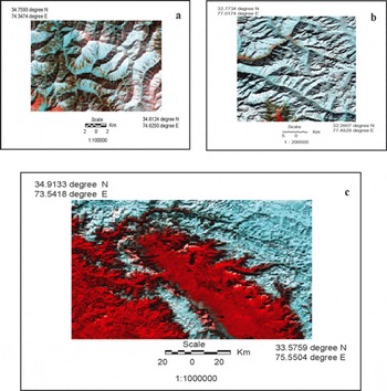
Fig. 1. False-colour composite (FCC) images of the three study areas on (a, b) AWiFS sensor (bands 2, 3 and 5) of 26 February 2005 and 8 January 2009 and (c) MODIS sensor (bands 3, 4 and 6) of 19 January 2005.
Satellite data
Two almost cloud-free scenes of the AWiFS sensor, on board IRS-P6 (RESOURCESAT-I), of 26 February 2005 (Fig. 1a) and 8 January 2009 (Fig. 1b), with spatial resolution of 56 m, and a third of the MODIS sensor, on board the Terra satellite, of 19 January 2005 (Fig. 1c) in spectral bands 3–7 at 500 m spatial resolution are used in the present work. The selection criteria for these scenes are acquisition at low solar elevation (45.5° for Fig. 1a, 33.4° for Fig. 1b and 33.5° for Fig. 1c) and availability of real-time in situ field data. The field observations of snow spectral characteristics were recorded in the complete solar wavelength range 350–2500nm using optical spectroradiometer at the time of satellite passes. These field results are used for validation with satellite-estimated spectral reflectance in AWiFS and MODIS spectral bands after different topographic corrections. The salient specifications of AWiFS and MODIS sensor bands are given in Tables 1 and 2.
Geometric corrections
The master data were prepared first by rectifying higher spatial resolution (23.5m) images of the Indian Remote-sensing Satellite (IRS) LISS-III (Linear Imaging Self-Scanning) sensor with the Survey of India (SoI) maps of different study areas. Thereafter, AWiFS images were georeferenced with LISS-III images. Similarly, moderate-resolution (500 m) MODIS data were rectified using medium-resolution (56m) AWiFS images. The image rectification was further refined using IL images. This step is essential to ensure that the satellite images used for topographic corrections match with topographical information generated using SoI maps to avoid erroneous results. The nearest-neighbor resampling method was used and the geolocation error of the model is about half a pixel.
Digital elevation model (DEM)
A DEM of the study area of AWiFS and part of MODIS was generated using a 1 : 50 000 toposheet at 40 m contour level. The Shuttle Radar Topography Mission (SRTM) data of the DEM at 90m spatial resolution were also used for certain regions of the study area on MODIS images. The non-linear interpolation function is used for three-dimensional (3-D) surface generation. The grid resolution of the DEM is 6 m and 90 m which were further resampled at 56 and 500 m to make it equal to the grid resolution of AWiFS and MODIS satellite images respectively. Thereafter, the DEM was used to generate terrain parameters for topographic models using ERDAS Imagine 8.7.
Testing and Evaluation
Qualitative visual performance
The performance of the following algorithms for topographic corrections was analysed qualitatively and quantitatively: C-corrections, Minnaert methods (including the slope in Equation (5)) and slope-matching technique. The values of the coefficients estimated for C-corrections (cλ), Minnaert constant, k(λ) and slope-matching parameter (methods) (Cλ) are given in Table 4. The values of these coefficients are different for different satellite data in different spectral bands of AWiFS and MODIS, thereby confirming the necessity for their estimation for each image in view of varying illumination. The Minnaert constant shows completely non-Lambertian behavior for the Himalayan terrain.. The comparative visual analysis for one of the results of AWiFS (8 January 2009) obtained using different topographic methods (using Equations (3–6)) is shown in Figure 2. The topographic results obtained using the slope-matching method for AWiFS (26 February 2005) and MODIS (19 January 2005) are also shown in Figure 3. The visual effect is more impressive in slope match (Figs 2d and 3a and b) as compared to other results (Fig. 2a–c). The 3-D relief effect is minimized and shows flat representation of the terrain. The appearance of land cover becomes much more independent of topography than in the original uncorrected bands (Fig. 2a). The topographical results obtained using C- and Minnaert corrections do not improve the visual results, and 3-D relief effects are still evident. The results of the first stage of the slope-matching method are shown in Figure 4. The best 3-D visual appearances are observed on the MODIS imagery (Fig. 4c) as compared to AWiFS imagery (Fig. 4a and b) in first-stage results. The shadow is almost completely removed. The geomorphology and terrain features of the image are also enhanced as compared to the original image. In order to confirm the actual land cover after topographic corrections, especially in shady areas, the results are compared with the normalized difference snow index (NDSI). NDSI is estimated for AWiFS and MODIS (Reference Hall, Riggs and SalomonsonHall and others, 1995), and the thematic results are shown in the Figure 5. NDSI can retrieve information under mountain shadow. Its values vary from –1 to +1 and are positive for snow (white area in Fig. 5) and negative for non-snow area (black colour in Fig. 5). The comparative analysis of Figure 3 with Figure 5 shows that slope matching is the only method that retrieves the true information under shadow.
Fig. 2. Topographically corrected image of AWiFS: (a) C-correction; (b) Minnaert correction (Equation (4)); (c) Minnaert method (Equation (5)); and (d) slope match method.
Fig. 3. Topographic correction results by slope match method: (a) AWiFS, 26 February 2005; (b) MODIS, 19 January 2005.
Fig. 4. First-stage normalization image of slope match for visual interpretation of topographical features: (a, b) AWiFS and (c) MODIS.
Fig. 5. NDSI image showing snow area (white: NDSI > 0.6): (a) AWiFS, 26 February 2005; (b) AWiFS, 8 January 2009; and (c) MODIS, 19 January 2005.
Table 4. Coefficients for different topographic normalization models. Values are in AWiFS and MODIS band ascending order
Quantitative analysis
To evaluate the model quantitatively, firstly, we estimated the typical mean values of spectral reflectance of the snow samples from the radiometrically corrected (atmospheric correction and topographic normalization) and uncorrected images on the south (Sun-facing) and north (shady slopes) aspect in all AWiFS and MODIS bands as shown in Table 5. These results suggest that in the uncorrected images the apparent reflectance of snow on the shady slope is very low. This is obviously untrue since it is known that snow reflectance is very high in visible bands (Fig. 6). The low values can be attributed to shadowing effects on shady slopes. Secondly, if the topographic corrections are successful, the mean values of snow samples on the shady slopes (north aspect) should increase while those of sunny slopes should decrease. It is observed from Table 5 that, although all the topographic methods satisfy the above-mentioned criterion, the corrected values of reflectance for snow samples on the north aspect using C- and Minnaert corrections (including slope) are not comparable to the typical true values. If the shady and Sun-facing slopes have the same snow cover, the spectral reflectance of snow should be homogeneous. After atmospheric correction and topographic normalization, the snow reflectance on shady slopes is observed to show the true situation in slope-matching method only.
Fig. 6. In situ observations of spectral reflectance characteristics of pure snow at the time of satellite pass.
Table 5. Mean values of spectral reflectance of snow samples in AWiFS and MODIS bands, and values on the north and south aspects of an entire image
Validation
Topographical results for all the images are validated with in situ observations of spectral reflectance of snow recorded at different geolocation points using the optical spectroradiometer at the time of satellite pass in real time in the wavelength range 350–2500nm. The mean curves for three different dates of satellite pass are shown in Figure 6. The mean values from the field observations (Fig. 6) were obtained in the respective spectral bands of AWiFS and MODIS (Table 6). The comparison of field results with satellite-estimated reflectance values before and after the topographic corrections in Table 6 shows that all the methods except slope match underestimate the reflectance values. The inference from Table 6 is that the mean reflectance values of snow samples of an entire image and on the south and north aspects are comparable only in slope-matching method. This is possible only when information is retrieved under the shadow area.
Table 6. Validation of topographic normalization models with field results of spectral reflectance using spectroradiometer
Graphical analysis
The topographic corrections were also evaluated using graphical analysis of spectral reflectance with IL both before and after the corrections. The visible band reflectance of AWiFS (B2) and MODIS (B3) with IL are shown in Figure 7. The results suggest that reflectance changes with IL for the uncorrected image of AWiFS (Fig. 7a and e) but, after the topographic corrections are carried out, it remains constant with different values of IL. On the other hand, uncorrected reflectance in MODIS with different values of IL (Fig. 7i) does not show much variation with IL. These results suggest that MODIS imagery does not require topographic corrections since all the topographic models show satisfactory results for Himalayan terrain. By contrast, the integrated analysis of different topographic results as discussed earlier suggests that the slope-matching method is most suitable for Himalayan terrain and that topographic corrections are required for MODIS images and for visual interpretation and quantitative analysis of snow-cover applications.
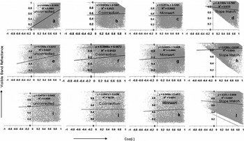
Fig. 7. Graphical analysis of reflectance in visible band with illumination before and after topographic corrections using different methods: (a–d) AWiFS, 26 February 2005; (e–h) AWiFS, 8 January 2009; and (i–l) MODIS, 19 January 2005.
Conclusions
The present paper discusses qualitative and quantitative analysis of different topographic correction methods on AWiFS and MODIS satellite data. The first stage of the slope-matching method shows excellent 3-D terrain geomorphology by removing the topographical relief effect, especially in MODIS data. Three-dimensional relief effects are minimized only in the slope-matching method and show flat representation of the terrain. The C-correction and Minnaert methods are not very successful and produce poor results. The Minnaert method also shows completely non-Lambertian behaviour of the Himalayan terrain. The slope-matching method has advantages in the true quantitative retrieval of spectral reflectance, especially in shady area, compared to C-correction and Minnaert methods.
Acknowledgements
The authors thank R.N. Sarwade (Director SASE) for kind permission to submit the paper. Thanks are also due to the internal SASE committee for reviewing it before submission. We acknowledge the valuable critical review by two anonymous reviewers for significant improvement of the paper.


