


INTRODUCTION
Global efforts to eradicate wild polioviruses continue, with types 1 and 3 wild polioviruses remaining endemic in four countries (Nigeria, India, Afghanistan, Pakistan) and causing fewer than 2000 global cases of paralytic polio annually [Reference Dutta1]. While wild polioviruses circulate in these areas, the rest of the world must continue to keep polio vaccination levels very high [Reference Thompson and Duintjer Tebbens2], due to the risk of outbreaks in susceptible people in polio-free countries. In addition, post-eradication policy planning must anticipate that outbreaks (defined as one or more cases of paralytic polio) will occur after the successful disruption of wild poliovirus transmission [Reference Thompson3, Reference Duintjer Tebbens4], largely due to the risks of circulating vaccine-derived polioviruses (cVDPVs) [Reference Duintjer Tebbens5]. Most people infected with poliovirus do not show any symptoms, which necessitates modelling the transmission of infections [Reference Duintjer Tebbens5], but about 1/200 susceptible people becomes paralysed from a wild poliovirus infection [Reference Sutter, Kew, Cochi, Plotkin, Orenstein and Offit6–Reference Dowdle and Birmingham8]. The costs of outbreaks include both health costs experienced by paralysed individuals plus the impacts on their families, and the financial costs associated with treating patients and responding to the outbreak with vaccine campaigns to reduce transmission [Reference Duintjer Tebbens9–Reference Prevots, Ciofi degli and Sallabanda11]. Two vaccines provide protection from disease (paralytic poliomyelitis), but incomplete protection from infection: live oral poliovirus vaccine (OPV) and inactivated poliovirus vaccine (IPV). OPV represents the vaccine of choice for the Global Polio Eradication Initiative because of its low cost, ease of administration, induction of mucosal immunity, and ability to provide secondary protection (i.e. spread to contacts). However, OPV can cause vaccine-associated paralytic polio in rare cases and lead to outbreaks with cVDPVs in populations with large numbers of susceptibles, and consequently following the successful eradication of wild polioviruses global health leaders plan to eliminate the use of OPV [12]. Minimizing the risks of outbreaks will require coordination of OPV cessation, creation of a global vaccine stockpile, and development of specific plans for outbreak response [Reference Thompson and Duintjer Tebbens13, Reference Duintjer Tebbens14]. Many countries will also consider switching from OPV to IPV because it carries no risk of vaccine-associated polio paralysis, but IPV represents a relatively expensive choice and its ability to prevent poliovirus transmission in some settings (notably low-income areas with relatively poor hygiene and inadequate health systems) remains uncertain [Reference Thompson3, Reference Duintjer Tebbens4].
Previous work by two of the authors (R.D.T. and K.T.) developed a differential equation-based (DEB) model [Reference Duintjer Tebbens9] to explore the dynamics of poliovirus infection outbreaks and response strategies [Reference Thompson, Duintjer Tebbens and Pallansch15]. This model yields useful insights, but we recognize the opportunity to address different questions using a stochastic, individual-based (IB) (or agent-based) modelling approach that explicitly considers the network structure of individuals and the stochastic interactions between individuals.
Previous studies identified the selection of the network structures as a critical assumption [Reference Colizza16–Reference Rahmandad and Sterman22], and show that DEB and IB models can yield different insights, in part due to the differences in their abilities to capture network structures and population heterogeneity [Reference Rahmandad and Sterman22]. In contrast to the assumption of homogenous mixing in DEB models, IB models typically require a network structure that governs the interactions of individuals. Analysts must identify links between individuals (nodes in the network) that specify ‘who acquires infection from whom’ (WAIFW) to mimic the interaction patterns of individuals in a real population [Reference Brisson23, Reference Mossong24].
We identified five major theoretical network structures in the literature: fully connected, random [Reference Erdos and Renyi25], small-world [Reference Watts and Strogatz26], scale-free [Reference Barabasi and Albert27], and all-in-range (local) [Reference Ferguson, Donnelly and Anderson28]. Figure 1 provides a graphical representation of example networks from each category. The literature also includes examples of empirical networks, which seek to closely mimic individual contact patterns determined through: (1) contact tracing of individuals [Reference Eames, Read and Edmunds29, Reference Friedman30], or (2) capturing physical locations (mixing-sites) in which individuals spend time with others (e.g. schools, workplaces, recreation centres, shopping malls) that determine interactions based on emerging co-location patterns [Reference Longini31].
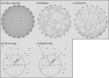
Fig. 1. Examples of the five different theoretical network structures, with each network including 20 individuals (nodes) (n=20) and each node connecting to six other nodes on average (K=6). The initial layouts of nodes in the networks shown in panels (a)–(c) appear as a ring, but the reasonable representation of the initial structure for the networks shown in panels (d)–(e) require random distribution of nodes. The network obtained in panel (e) results from rewiring the network in panel (d) as described in the text.
Despite the importance of network structure, IB models remain limited with respect to the available information about WAIFW in real populations [Reference Halloran32]. Consequently, identifying the critical network parameters that influence outbreak dynamics is essential to develop appropriate IB models to address policy questions and guide data collection [Reference Mossong24, Reference Zagheni33]. This study describes our efforts to develop an IB model to characterize poliovirus outbreaks at the level of interactions among individuals and explore the impacts of network choices. The IB model explicitly captures immunity states and transition rates similar to those developed earlier [Reference Duintjer Tebbens9], but focuses on stochastic attributes of state transitions and the impact of different network structures on the transmission process.
METHODS
We developed an IB model for a hypothetical outbreak in a low-income country setting, corresponding to the prospectively modelled outbreak in Figure 2 of Duintjer Tebbens et al. [Reference Duintjer Tebbens9]. The model assumes complete eradication of wild polioviruses and starts the outbreak with a single poliovirus introduction 5 years after cessation of all polio vaccinations. We explored multiple different network structures, including the five theoretical networks shown in Figure 1 and several empirical mixing-site networks. Figure 2 shows the basic structure of the immunity states from the DEB model [Reference Duintjer Tebbens9] and individual state transitions in our IB model for poliovirus infections. The 13 different states modelled capture infectible people (top row), people with latent infections (second row), infected people (third row), and removed people (bottom row). The model captures four different types of immunity: (1) ‘fully susceptibles’ – never exposed to live or killed poliovirus, (2) ‘recent live’ partially infectibles – individuals recently infected with live poliovirus, (3) ‘historic live’ partially infectibles – individuals historically, but not recently, infected with live poliovirus, and (4) ‘IPV’ – individuals never infected with live poliovirus but vaccinated with IPV [Reference Duintjer Tebbens9]. Although not shown in Figure 2, the DEB and IB models also include 25 different age groups [Reference Duintjer Tebbens9], which influences the network patterns in mixing-site settings. We define inputs to the IB model with a fully connected network parallel to the DEB model and keep the same basic reproduction number (R 0) across both models (see Appendix, available online). To model transmissions at the individual level rather than at the population level in the DEB model, we disaggregate the concept of R 0 into separate inputs for contact rate (C) and infectivity (i) of a contact (i.e. the probability of a contact leading to infection). Specifically, we start with the equation R 0=C * I * d for each type of infectious and infectible person, using d as the average duration of infectiousness for ‘fully susceptible’ individuals, and we calculate i based on an assumed value of C=5 contacts per day and the values of R 0 and d in the DEB model [Reference Duintjer Tebbens9]. The choice of C does not impact R 0 as long as i adjusts to C. We confirmed that we obtained the expected R 0 in the simulations by calculating the average number of individuals directly infected by a single infectious individual introduced in a fully susceptible population (see online Appendix).
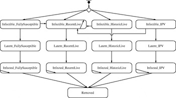
Fig. 2. Immunity and infectiousness states based on [Reference Duintjer Tebbens9] along with possible transitions in the IB model.
Consistent with the DEB model [Reference Duintjer Tebbens9], which begins with a population immunity profile that distributes members in the population to appropriate initial immunity states, the IB model begins by assigning each individual to an initial state as susceptible or partially infectible. The initial population immunity profile follows the projected age distribution for low-income countries and places all children aged <5 years in the ‘infectible-fully susceptible’ state given the assumption of cessation of all polio vaccination 5 years prior to the outbreak [Reference Duintjer Tebbens9]. We assigned members of the population aged >5 years to the ‘infectible-historic live’ or ‘infectible-fully susceptible’ state according to assumptions about the historical OPV vaccination rates [Reference Duintjer Tebbens9]. Given the assumed lack of IPV or OPV use prior to the outbreak, none of the individuals start in the ‘infectible-IPV’ or ‘infectible-recent live’ states.
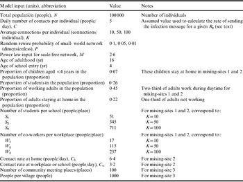
We compared the transmission dynamics across all five of the major theoretical network categories from the literature and three empirical mixing-site networks. The top part of Table 1 describes the construction rules applied to create the theoretical networks, and the bottom part provides the assumptions used to create three mixing-site networks, which reflect possible scenarios to bring individuals into contact at identifiable locations (e.g. home, work, school). Although modelling real population interactions using mixing-sites requires significant data and detailed information about types of contacts leading to infection [Reference Eubank34], we determined that in the absence of specific data we could still learn about how mixing-site networks function by considering the scenarios in Table 1. We chose to model two basic types of empirical mixing-site networks: one that focuses on workplaces and schools as hubs of transmission within a large population (mixing-sites 1 and 2) and one that focuses on modeling the population as a collection of villages from which individuals connect periodically (mixing-site 3). While the selection of network type and model inputs may lead to different results and infinitely many options exist for developing empirical network strucutres, we focused our analysis on demonstrating the differences between a range of typical empirical and theoretical networks. In order to explore networks consistently, we used the same total number of individuals (nodes, agents) (N), and the same average number of connections per individual (K) when comparing networks that use K as an input. However, recognizing the uncertainty in network parameters, we repeated comparisons for three different values of K. Table 2 summarizes the specific input values used for the networks.
Table 1. Summary of model inputs for an individual-based model that differ from those used for the differential equation-based (DEB) model [Reference Duintjer Tebbens9] via different types of social contact networks
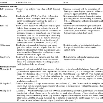
Table 2. Summary of model inputs for the IB model that differ from those used for the DEB model [Reference Duintjer Tebbens9] for the different networks structures described in Table 1
Each simulation of the IB model begins by creating a population of N=100 000 individuals. The IB model distributes the individuals into their age and initial immunity groups and then sets up the chosen network structure to connect individuals using a construction rule. During the simulation births occur and susceptible newborns enter the network with connections created by applying the same construction rule used to create the initial network, with the net effect of increasing the potential number of people who could become infected to >100 000. Consistent with the original model designed for outbreaks of short duration [Reference Duintjer Tebbens9], this model ignores deaths. Thus, the network is dynamic in the sense that new individuals get added and wired to the rest of the population, but the existing connections do not change dynamically (e.g. because of self-quarantine).
We introduce the first, randomly selected, infectious individual (patient zero) into the population at time zero of each simulation to initialize the infection process. The outbreak may die out if the patient is removed before infecting others. However, an outbreak occurs in the population when the imported poliovirus establishes effective transmission in individuals (presumably primarily via the faecal–oral route and possibly to some extent via the oral–oral route [Reference Melnick, Evans and Kaslow35]) and infects enough people to cause at least one paralytic case [Reference Duintjer Tebbens9]. Infection depends on the existence of connections between infectious and infectible individuals in the network and the contact rate (C). Not every contact between an infected individual and an infectible individual leads to infection, and the probability of infection following contact (i) depends on the individual's immunity state.
We performed repeated analyses for three different average numbers of connections per individual (K=10, 50, 100) to explore a range given limited knowledge about how contacts lead to poliovirus transmission. We also explored all five of the theoretical networks in the top part of Table 1, and for the small-world network, we explored the impact of three different values for the probability of random rewiring of the local links (P=0·01, 0·05, 0·1), which makes a total of seven simulated theoretical networks. We note that the random, small-world(s), and all-in-range networks represent a continuum of different levels of clustering and average distances between nodes. The clustering and distances decrease as we increase P, because a small-world network with P=1 yields a random network, while setting P=0 yields an all-in-range network. To facilitate some comparison between the seven simulated theoretical networks and the three simulated mixing-site networks, we selected the number of co-workers per workplace (W) and students per class (S) such that time-weighted average connections per person (K) remain the same as the value used for other network settings, noting that K does not exist for the fully connected and mixing-site 3 networks. We used the same contact rate (C) for all networks, except for mixing-site 2, for which we used twice the contact rate for home than that for schools and workplaces to explore the impact of differential contact intensity in different locations while also maintaining the same R 0, as noted in Table 2.
We projected the trajectory of potential polio outbreaks and we compared the results across different network and model inputs using the AnyLogic™ (XJ Technologies, Russia) simulation environment. We recorded an outbreak upon detection of the first paralytic case, which occurs stochastically in about 1/200 infections of ‘fully susceptible’ individuals [Reference Duintjer Tebbens9]. We tracked the trajectory of the outbreak until it finished (i.e. no latent or infected individuals remain in the population) or until day 2000, whichever comes first. Each simulation started with construction of a new network consisting of 100 000 initial individuals, and a randomly selected patient zero. Due to the stochastic nature of the simulations, we ran 100 simulations for each of the 10 simulated networks for three different values of K (for networks that include K) for a total of 26 combinations (i.e. the fully connected and mixing-site 3 networks do not include K). During the simulation, we captured the following metrics:
• Die-out fraction (dimensionless). The fraction of simulations that do not lead to an outbreak, defined as detection of a paralytic case.
• Detection day (day). The day that the first paralytic case occurs.
• Peak time (day). The day with the highest number of infections observed within the duration of poliovirus diffusion.
• Epidemic duration (day). The time it takes for the outbreak to end (i.e. the time until no latent or infectious individual remains), which we record as >2000 days if transmission continued beyond the maximum simulation length.
• Number of infections (number of people). The cumulative number of people who become infected and get removed (recover or die from the infection) at the end of the simulation.
• Number of paralytic cases (number of people). The total number of paralytic cases accumulated by the end of the simulation.
• Peak infections (number of people). The number of people infected at the peak time.
If the event captured by the first metric occurs (i.e. the transmission of infection dies out and does not lead to an outbreak), then the remaining metrics do not provide interesting or meaningful information, and consequently we report their results for only the subsets of 100 simulations that did not die out. For these metrics we found statistically robust means with the sample of 100 simulations. We performed 1000 simulations to characterize the die-out fraction results to obtain more statistically robust estimates.
RESULTS
Table 3 reports the results of the fraction of ‘die-out’ cases for different network structures and numbers of connections per individual (K) based on 1000 simulations. One of the significant advantages of IB models compared to a DEB model emerges simply from the ability to characterize the stochastic possibility of die-out. For example, although the comparable DEB model with the relativley high R 0 of 13 predicts an outbreak, the IB model with a fully connected network dies out by chance about 15% of the time, because the infection does not go beyond the first (few) patient(s) who get removed before infecting a larger population.
Table 3. Results of 1000 simulations of the fraction of ‘die-out’ cases (dimensionless) for 26 combinations of different network structures and numbers of connections between individuals (K)
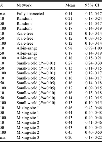
n.a., Not applicable.
Table 3 shows some differences in die-out behavior as a function of the type of theoretical network structure and number of connections (K). The random network for K=50 and K=100 behaves similarly to the fully connected network because relatively low clustering (i.e. neighbours of the same individual are not that likely to be connected to each other) leads to quick propagation of infection throughout the network, reducing the chance of die-out compared to a highly clustered population. However, with fewer connections per individual (K=10) we observe a larger die-out fraction (~21%), because the Poisson distribution of K implies a relatively large fraction of individuals with very few connections and thus a relatively lower probability of pushing the virus beyond patient zero. Notably, if patient zero is one of the relatively poorly connected individuals, then the outbreak is more likely to die out. For the scale-fee network, we see a relatively small die-out fraction (~10–13%), which indicates that the few ‘hubs’ of highly connected individuals serve as relatively effective spreaders, because they connect most people in the population with small distance between individuals. Thus, although the fixed number of connections (K) requires the existence of many individuals with relatively few connections to average out the hubs (for all three values of K), in most cases patient zero infects a hub directly, and then the hubs infect each other and much of the rest of the population fairly quickly. The all-in-range network behaviour depends heavily on K. With K=10, only a small number of outbreaks occurred in the 1000 simulations, given the highly localized nature of interactions, which implies that nearly all of the infections died out prior to causing a paralytic case. Individuals in the all-in-range network share many connections with their neighbours, which lessens the impact of infection of two connected people since they probably share many contacts, and this overlap reduces their ability to transmit the virus to new people. However, as K increases, the all-in-range network goes through a phase shift, in which the larger radius of interaction makes the progression of virus viable and die-out drops to ~18%. For the small-world network, we generally see low die-out fractions (i.e. 12–16%), because long-range connections seed the virus in multiple locations and therefore reduce die-out. However, for the small-world network with P=0·01 and K=10, we see the same type of phase shift as occurred with the all-in-range network with K=10, which appears consistent with previous observations of such a phase transition [Reference Watts and Strogatz26].
For mixing-sites 1 and 2, which move individuals between home and work or school, we observed a significant increase in the fraction of simulations that die out (i.e. 40–50%) compared to what we found for most of the theoretical networks (i.e. 12–19%, with the notable exceptions of the results of the random, all-in-range, and small-world networks with K=10). We believe that this may occur because: (1) most contacts happen in highly clustered family units, which limits transmission beyond the family in the relatively fewer contacts between infectious members of the household and their co-workers/schoolmates, and (2) one-third of adults and young children stay at home, which reduces opportunities for transmission. The young age of fully susceptibles (with relatively higher infectivity) further increases the importance of the mixing-site dynamics. In contrast, the contact pattern in mixing-site 3, which is independent of K, shows a much lower die-out fraction (~20%). For mixing-site 3, people connect to each other across 1000-member villages, in which the virus can spread with no restriction if the virus gets transmitted during the limited weekly mixing time at community centres (e.g. markets or places of worship).
Table 4 shows the results for the metrics that provide insights about the nature of the simulated outbreaks that do not die out, and Figure 3 a provides a visual representation of the outbreak dynamics by showing the number of infected fully susceptibles as a function of time. The detection day of the first paralytic case provides an indication of the speed of the transmission of infections in ‘fully susceptible’ individuals under different network structures. The peak day provides an indication of the overall speed of transmission in the whole population. The outbreak duration provides insight about how quickly the infection passes through the entire population, and indicates whether the outbreak could continue for >2000 days absent intervention. The total number of infections serves as an indicator of the impact of the network on the extent to which infection spreads through the population. The peak infections allow us to see the maximum numbers of people infected simultaneously, which reflects the maximum intensity of the transmission of infection under the different types of network structures. The last column of Table 4 provides the estimated number of paralytic cases, which would typically represent the only observable outcome, and Figure 3 b shows large differences in the accumulation of these cases over time for various network structures.
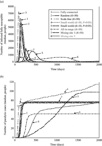
Fig. 3. Visual representation of the behaviour of outbreaks for eight selected simulated networks as a function of time: (a) number of infections occurring in fully susceptible people as a function of time, and (b) accumulated number of paralytic cases as a function of time.
Table 4. Results of 100 simulations for outbreak metrics for 26 combinations of different networks and values of K based on the subsets of simulations in which outbreaks did not die out (robust simulation mean, in units indicated for each metric)
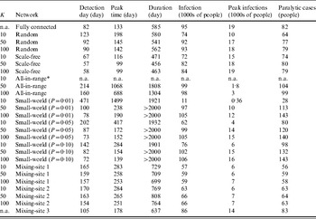
n.a., Not applicable.
* No outbreaks observed in 100 simulations.
Table 4 shows some important differences in the outbreaks depending on the assumptions about the network. In contrast to the stochastic variation that we observed related to die-out fractions (Table 3), we observed negligible stochastic variation across for the outbreak metrics in Table 4 relative to the number of significant figures supported by the model, and consequently Table 4 reports only the robust mean values for these metrics. On average, the outbreaks that occur with the fully connected network take off relatively quickly (e.g. detection day=82, peak time=133, compared to detection day=78, peak time=128 for the DEB model [Reference Duintjer Tebbens9]). At its peak, the typical outbreak with the fully connected network involves >18 000 infected individuals and the rapid spread of infection limits the overall duration of the epidemic to 585 days on average, with >95% of the population becoming infected and an average of 82 paralytic cases. The results with the random network show similar behaviour, although the average outbreak occurs relatively later (detection day=123), proceeds more slowly (peak time=178), and leads to fewer numbers of infected individuals (74% of the population becomes infected) and paralytic cases (64). For the scale-free network, we see a very fast take-off for the outbreak, which increases the peak infections and reduces the duration of the outbreak. As noted above, patient zero typically infects a hub directly or with one degree of separation in the scale-free network, which leads to rapid infection of all of the hubs, which then infect most of the population. However, the existence of some poorly connected individuals means that the outbreak fails to reach all of the individuals, such that between 72–84% of the population becomes infected, depending on K. Higher K values appear to speed up the outbreak slightly, but do not have a large impact because enough hubs exist with K=10 to start and support widespread transmission. For the all-in-range network, the outbreak depends heavily on K, with essentially no outbreaks for K=10, and relatively slow outbreaks for K=50 and K=100 that move through the population in a wave-like progression from the location of patient zero outwards. Given the slower diffusion with K=50, this setting leads to larger peak time, detection date, and duration than does the setting with K=100. Notably, slower diffusion actually increases the total number of infections because it extends the epidemic to affect more newborn babies over time. For the small-world network, we generally observe high numbers of infections, except for the network with mainly local connections for K=10 and P=0·01. We observe the highest numbers of infections and paralytic cases for the all-in-range network with K=50, 100 with outbreaks that continue beyond 2000 days in most cases, because the slow transmission that results from largely local links (see the large peak time) essentially matches the speed of entry of fully susceptible newborns.
For mixing-sites 1 and 2, the outbreaks that take-off appear relatively insensitive to K and C. For these mixing-site networks, we see a slow outbreak (e.g. later detection day and peak times than most other network types) that affects the majority of the population before ending after about 700–770 days. Shifting the weight of the contacts more towards homes (mixing-site 2) leads to slightly higher numbers of infections and faster outbreaks, presumably because household links act as a bottleneck on transmission for mixing-site 1. By increasing the relative speed of transmission in the home for mixing-site 2, the one-third of household members who do not mix outside of the home become more prone to infection. In contrast to mixing-sites 1 and 2, the contact pattern in mixing-site 3 allows infection to spread through the whole population, only slightly slower than the fully connected network, with the majority of people becoming infected at the end of the outbreak, which occurs within a few months.
DISCUSSION
Previous research demonstrates the importance of structural and model input assumptions for other diseases [Reference Highfield36, Reference Viet, Fourichon and Seegers37], but this paper presents the first IB model for polio outbreaks. By developing this model, we created the opportunity to both represent the stochastic nature of polio outbreaks and consider the impact of different network structures to model heterogeneous human interactions. With realistic network structures, IB models may show behaviours that differ significantly from the parallel DEB models, and offer opportunities to characterize interventions that target specific types of individuals or parts of networks. We anticipate that IB models could play a valuable role in evaulating different polio outbreak response strategies, such as comparing mass vaccination and ring vaccination options.
Despite the potential uses of IB models, our results suggest important considerations. The computation time, which includes both network set-up and transmission dynamics, increases significantly with population size. Notably, the scale-free network we modelled required about 30 min per simulation just to set up the network on an Intel Core™ 2 CUP 6400 @ 2·13 GHz desktop. The computation times for transmission simulation and data recording scale approximately linearly with population size. Thus, simulating very large populations (e.g. millions of individuals) would require specialized computer clusters, although improved hardware and algorithms continue to reduce computational barriers [Reference Halloran32, Reference Eubank34, Reference Colizza38]. The necessity of conducting comprehensive sensitivity analyses to characterize the impacts of uncertain assumptions adds another dimension of computational time. However, sensitivity analyses reveal critical insights and help analysts address the false certainty and precision projected through the use of detailed IB models [Reference May39], and our analyses suggest that the level of stochastic uncertainty may differ across outcome metrics. We note that the closed-source nature of the AnyLogic modelling tool makes it difficult to evaluate the impact of software algorithms and programming choices that could affect the results. We do not believe that choosing a different software program would change the insights that we obtained here related to our comparisons between networks, but we mention this as a limitation because we only compared our results to the previous DEB model and we did not compare results between open and closed-source software tools.
Our analysis of various options for network structures, which underlie all IB models, highlights the importance of choices related to both model structure and inputs. Previous studies indicate that scale-free and small-world networks might make the most sense for infections transmitted through individual-to-individual networks, like sexually transmitted diseases [Reference Donnelly and Cox40, Reference Anderson, Gupta and Ng41]. In contrast, mixing-site networks may provide a better representation for airborne diseases such as flu [Reference Mossong24, Reference Longini31, Reference Ferguson42]. For poliovirus infections, we expect that using mixing-sites may also offer the best strategy, but even with a limited set of scenarios for these we found potentially large differences in the behaviour of outbreaks. In this regard, we expect that improvement of IB models for polioviruses will require a more detailed understanding of the processes that create WAIFW patterns in specific populations of interest, and that additional insights about the relative importance of faecal–oral vs. oral–oral transmission pathways may also help to influence choices about network structures and contact rates both within and between mixing-sites. Epidemiological investigations could provide important insights that would significantly improve our ability to model outbreaks. As long as live polioviruses continue to circulate, the opportunity exists to better characterize the role of potential mixing-sites in poliovirus transmission in low-income countries, including markets, schools, places of worship, sewage, rivers, and workplaces. The role of migrant populations also represents an important consideration, and data on population movement in countries of highest concern for poliovirus transmission could provide significant insights with respect to developing appropriate networks. While polioviruses can spread over long distances [43], the relative frequency of short-distance to long-distance poliovirus infectious contacts remains unknown and requires further investigation.
Several observations also suggest the need for additional development of the IB model. First, we observed persistent transmission as a result of a re-introduction in small-world networks, which suggests the need to include age-dependent mortality rates and waning of immunity. Second, if we seek to use the model to evaluate specific outbreak response strategies, then we would need to use serotype-specific model inputs and explicitly characterize the transmission and evolution of OPV viruses to address questions related to the development of cVDPVs. Thus, although this work suggests that IB modelling offers an important opportunity to better characterize the actual dynamics of the spread of infection, using IB models appropriately for polio outbreaks will depend on obtaining high-quality information about the nature of polioviruses, immunity, and social interactions.
NOTE
Supplementary material accompanies this paper on the Journal's website (http://journals.cambridge.org/hyg).
ACKNOWLEDGEMENTS
The authors received support from a grant to Kid Risk, Inc. from the World Health Organization Polio Research Committee. The findings and conclusions in this report are those of the authors and do not necessarily represent the views of the World Health Organization.
DECLARATION OF INTEREST
None.


