


INTRODUCTION
Dengue is a disease caused by a virus of the family Flaviviridae and is mainly transmitted by the mosquito Aedes aegypti, which is found in tropical and subtropical regions worldwide [Reference Gubler and Clark1, Reference Gubler2]. In recent years, transmission has increased mainly in urban and semi-urban areas and has become a major international public health concern [3]. According to the WHO [4], more than 2·5 billion people – representing over 40% of the world's population – are at risk of dengue. There are four distinct serotypes of dengue virus and recovery from infection by one serotype confers immunity to that particular serotype [3]. There is cross-immunity to other serotypes, but this is only partial and temporary [3]. Subsequent infections with other serotypes increase the risk of developing a more severe form of dengue called severe dengue (formerly known as dengue haemorrhagic fever) [3]. Currently there are no specific treatments and there is no vaccine to protect against dengue, although there are ongoing trials on vaccines which give partial protection against some serotypes [Reference Webster, Farrar and Rowland-Jones5, Reference Sabchareon6]. The usual methods to control or prevent the spread of the disease involve vector control interventions such as removal of artificial man-made larval habitats, coverage of domestic water storage containers and insecticide space spraying [3]. All these control interventions are supplemented by the use of personal household protection such as tulles, coils and window screens to avoid contact with mosquitoes [4]. Since the publication of the first model concerning dengue transmission [Reference Newton and Reiter7], several models have been developed involving different mathematical approaches or taking into account different possible aspects of the disease: constant human population and variable vector population [Reference Esteva and Vargas8], variable human population size [Reference Esteva and Vargas9], vertical and mechanical transmission in vectors [Reference Esteva and Vargas10], seasonal parameters and presence of two simultaneous dengue serotypes [Reference Bartley, Donnelly and Garnett11], age structure in the human population [Reference Pongsumpun and Tang12], presence of multiple serotypes [Reference Feng and Velazco-Hernandez13–Reference Wikramaratna19], use of remote-sensing data [Reference Tran and Raffy20], competition for female mating between wild and released mosquitoes [Reference Atkinson21], spatial heterogeneity [Reference Favier22], mosquito dynamics [Reference Focks23], spatial dynamics of the disease [Reference Otero and Solari24, Reference de Castro25], vaccination [Reference Supriatna, Soewono and vanGils26], implementation of realistic distributions for the duration of the incubation periods [Reference Otero27], human movement [Reference Adams and Kapan28, Reference Barmak29] and impact of vector control interventions [Reference Newton and Reiter7, Reference Burattini30–Reference Oki32].
In this work we present an improvement of a previous model [Reference Barmak29], in which the spatio-temporal dynamics of the mosquito and humans are simulated simultaneously. This improvement allows us to study the impact of different health policies and vector control interventions, applied during an epidemic outbreak, as a result of its evolution. We consider measures such as: restriction of human movement, human isolation strategies, vector space spraying and combined strategies.
METHODS
Model
Vector dynamics
From a biological point of view we consider six different stages for the mosquito: three immature stages: eggs E, larvae L and pupae P, and three adult stages: adult females in their first gonotrophic cycle (A1), females in subsequent gonotrophic cycles (A2) and flyers (F). The model is spatially explicit being the mosquito and human populations located in square patches (blocks). We consider that mosquitoes disperse in search of oviposition sites [Reference Edman33, Reference Bergero34]. Having completed the gonotrophic cycle after a blood meal the mosquito can fly to adjacent patches following a diffusion-like process [Reference Otero, Schweigmann and Solari35].
From an epidemiological point of view we divide the adult female vector population in three compartments representing the disease status: susceptible (S), exposed (E) and infectious (I). In this work we consider that only one serotype of the dengue virus is circulating.
The female mosquito requires a blood ingest to complete its gonotrophic cycles. In this process a susceptible mosquito may ingest viruses with their blood meal by biting an infectious human (vector contagion). The mosquito becomes exposed and the viruses develop within the vector during its extrinsic incubation period (EIP). After an EIP of 10 days the female mosquito becomes infectious and the viruses are injected into the bloodstream of other humans with the saliva of the mosquito in later blood meals (human contagion).
According to the biological stages of the mosquito and its status with respect to the disease, 28 different subpopulations for the mosquito are taken into account. Three immature subpopulations: eggs E, larvae L and pupae P and 25 adult subpopulations: susceptible female adults not having laid eggs A1, susceptible flyers F s, exposed flyers during the ten different days of the EIP, F e(k) with 1⩽k⩽10, infectious flyers F i, and female adults having laid eggs in the three disease compartments: susceptible A2s, exposed A2e(k), with 1⩽k⩽10 and infectious A2i.
Eggs, larvae, pupae and non-parus adults, A1, are considered susceptible. After a blood meal A1 becomes a flyer, susceptible F s or exposed F e(1) in the first day of EIP, depending on the disease status of the host bitten.
The evolution of the 28 subpopulations is affected by 68 different possible events, represented by arrows in Figure 1. Events occur at rates that depend on subpopulation values and some of them also depend on temperature, which is a function of time since it changes over the course of the year seasonally [Reference Otero, Schweigmann and Solari35, Reference Otero, Solari and Schweigmann36]. Hence, the dependence on temperature introduces a time dependence in the event rates. Table 1 summarizes the events and rates related to mosquito dynamics.

Fig. 1 [colour online]. Mosquito dynamics. Subpopulations and events of the stochastic model according to Table 1.
Table 1. Events related to mosquito dynamics. Event type and transition rates for the developmental model

The coefficients [Reference Otero and Solari24] are me, mortality of eggs; elr, hatching rate; ml, mortality of larvae; α, density-dependent mortality of larvae; lpr, pupation rate; mp, mortality of pupae; par, pupae into adults development coefficient; ef, emergence factor; ma, mortality of adults; cycle1, gonotrophic cycle coefficient (number of daily cycles) for adult females in stages A1; cycle 2, gonotrophic cycle coefficient (number of daily cycles) for adult females in stage A2; ovr, oviposition rate by flyers; disp, dispersal rate of flyers. A detailed description of the coefficient values can be found in Appendix B.
Host dynamics
Humans are considered at the individual level, i.e. with an individual based model (IBM) [Reference Otero27]. Epidemiologically, humans follow a susceptible (H S), exposed (H E), infectious (H I), recovered (H R) (SEIR) sequence. An individual becomes infected with the virus via the bite of an infectious mosquito, and enters the exposed stage during an intrinsic incubation period (IIP) that ranges between 1 and 8 days with a probability distributed with Nishiura's distribution for DENV-1 [Reference Nishiura and Halstead37]. Next, the individual becomes infectious for a viraemic period (VP) of 5 days and if bitten by susceptible mosquitoes he may infect the vector with a probability that depends on the viraemic day [Reference Nishiura and Halstead37]. Finally, the infectious human recovers and becomes immune to dengue for the rest of the simulation. In contrast with our previous works [Reference Otero27, Reference Barmak29], the evolution time of the infection in each human is asynchronous. This means that if someone is bitten at 14:00 hours and contracts the disease, a day is considered to have elapsed at 14:00 hours the following day.
From the point of view of human mobility, humans behave as in our previous work [Reference Barmak29]: i.e. half the population of each block stay at home all day, and the remainder go to work from 09:00 to 17:00 hours repeating the mobility pattern every day between the home and workplace. The workplace (block) is chosen at random at the beginning of the simulation from a random uniform distribution or a truncated Levy distribution [equation (1)] with parameters r 0 = 200 m, β = 2, κ = 1500 m [Reference Barmak29], which we will hereafter refer to as Levy 2.
 $$P(r){\rm \propto (}r{\rm} + {\rm} r_0 {\rm )}^{-\beta} {\rm exp(}-r/\kappa {\rm )},$$
where P(r) the probability of a human travelling a distance r and where r 0, β and κ are parameters that characterize the distribution. We take into account two mobility patterns to assess whether the qualitative results depend on the exact details of the mobility patterns.
Mathematical description of the stochastic model
The evolution of the mosquito subpopulations is modelled by a state-dependent Poisson process [Reference Ethier and Kurtz38, Reference Andersson and Britton39], where the probability of the state: [E, L, P, A1, A2s, A2e(1), …, A2e(10), A2i, F s, F e(1), …, F e(10), Fi] evolves in time following a Kolmogorov forward equation that can be constructed directly from the information collected in Table 1. The numerical implementation of the stochastic model is performed with fixed time steps of 2 h using a Poisson approximation [Reference Solari and Natiello40]. The day is divided into twelve 2-h subunits, for each 2-h step the model updates all mosquito subpopulations in each block according to the actions prescribed by the events presented in Table 1. The event of contagion of the vector is not calculated in the same way since vector contagion requires interaction between vectors and hosts.
The number of mosquito bites calculated is distributed randomly among all humans present at that time in the block. The bites made by infectious mosquitoes on a susceptible human may cause infection with a probability p mh = 0·75 (fixed throughout the whole simulation). Susceptible mosquitoes biting infected humans acquire the virus with probability p hm(j) [Reference Nishiura and Halstead37], where j is the viraemic day of the bitten human. It should be noted that mosquitoes are considered in compartments and we are unable to identify which mosquito has bitten which human. In each 2-h loop we count how many new exposed mosquitoes have resulted and place them in the compartment F e(1).
It is important to note that the present model differs from previous models [Reference Focks23, Reference Otero27, Reference Barmak29] in that the vector and host dynamics are modelled simultaneously. In the previous models a mosquito dynamic simulation was first run without taking into account whether the mosquitoes were infected or not. Other dengue models directly do not include a description of the vector's dynamics [Reference Newton and Reiter7–Reference Tran and Raffy20]. When mosquito dynamics are simulated independently of the disease, or not simulated at all, interventions on mosquito dynamics as a consequence of epidemic evolution cannot be properly simulated. An algorithmic description of the current model is given in Appendix A and a detailed description of the parameters of the model is given in Table 2 and Appendix B.
Table 2. Coefficients for the enzymatic model of maturation [equation (2)], where R D is measured in day−1, enthalpies are measured in (cal/mol) and temperatures T are measured in degrees Kelvin. A brief description of the enzymatic model of maturation can be found in Appendix B

Intervention measures
The use of insecticide spraying interventions (fumigations) to reduce vector populations, and the use of isolation strategies to reduce the number of individuals capable of transmitting the disease are common practices in dengue outbreaks [4]. We implemented some human isolation strategies and vector fumigations in our model in order to study the impact in the spread and evolution of dengue disease.
Movement restriction strategy
The movement restriction strategy requires that infectious people stay at home to recover and stop the 24-h cycle with 8 h at work. Although individuals remain at home, they may still be bitten by mosquitoes. Since dengue presents its first symptoms (fever) around the third day of the infectious state (VP), we applied this movement restriction strategy from the third day of the infectious state until the last (fifth) day. Since the exposed time is measured from the moment of the infective bite, people might become symptomatic while they are at work. In such cases, we allow that person to remain at work until returning home at the usual time; when he then starts obeying the movement restriction until the end of the infectious state.
Isolation strategy
It can be argued that the movement restriction strategy might not be enough to reduce or avoid the evolution of the disease, since vectors can still make contact with infectious humans and spread the infection. A better strategy would be the voluntary isolation of every person with any symptom compatible with dengue. In our model, people remained at home from the third day of the infectious state, as in the previous case, but on this occasion they were not bitten by mosquitoes. In practice, this could be achieved by keeping infectious people indoors and using window and door screens, mosquito nets, tulles, insecticide-treated bed nets, repellents containing DEET, IR3535 or Icaridin, mosquito coils, household insecticide aerosol products, insecticide vaporizers and long-sleeved clothes [3, 4]. The model does not discriminate between the different methods used to achieve isolation or the manner in which these are implemented, but accounts for the global effect as a whole. The contribution of each method of isolation is beyond the scope of this work. Although this strategy is harder to apply than the movement restriction strategy, it is still feasible. For this case, we performed three different simulations based on the isolation of infectious humans, i.e. 1 day only (day 3 of VP), 2 days (days 3 and 4) and 3 days (days 3–5).
Delayed measures
In the previous strategies we applied the intervention measures even for the index case. Nevertheless, control strategies cannot always be started from the beginning of an epidemic outbreak. Public health measures may follow the index case after some delay that depends on the preparedness of the society regarding the prevention of dengue outbreaks. We explored the effect of a delay in applying the 3-day isolation strategy. The delays considered are 14, 21, 60 and 120 days beginning from the day the index case became infectious.
Efficiency of isolation
It is expected that not all infected people will achieve isolation, either because they choose not to obey the strategy or because they do not know they were infected (subclinical cases with mild or no symptoms). To study the impact of such behaviour on the evolution of the disease, we ran simulations with different efficiencies of isolation: 90%, 70%, 50% and 25%. More explicitly, at the beginning of the simulation we selected randomly for each specific efficiency which individuals would be isolated or not regarding infectious cases.
Vector control interventions: fumigation
Interventions to control vector populations are a frequent approach to the problem. The most common, highly visible, method is the spraying of insecticides or fumigation during an outbreak [4]. Fumigation targets the adult mosquito population. In our simulations we considered that fumigation was effective over all (n = 25) adult mosquito subpopulations.
The procedure is as follows. Every time an infectious human appears at home, if not already tagged, his home block is tagged for spraying and is fumigated effectively T days later, irrespective of the number of new infectious humans that appear in that tagged block during that period of time T. Once the block has been fumigated, it is immediately untagged and a new infectious human can trigger a new fumigation in the same block.
It should be borne in mind that fumigation is not the perfect solution because of a variety of reasons [Reference Ekpereonne41]. We defined a global efficiency of fumigation, gef, for the simulations accounting for this fact. This efficiency is the probability of an adult mosquito dying immediately after a fumigation intervention has been performed in the block it inhabits. The adult surviving population was calculated considering binomial distributions with probability P = (1 − gef). It should be noted that we do not consider any residual effects of the insecticides, i.e. mosquitoes only die during the fumigation. To study the sensitivity to gef we used the following efficiencies 0·9, 0·5, 0·3, 0·1. The time elapsed between the case determining that the block should be fumigated (tagging) and the actual fumigation was set to T∈{3, 7} days.
Combined strategies (fumigation + isolation)
To maximize the effectiveness of the measures and to make them possibly more realistic in relation to the efficiencies needed to obtain useful results, we combined two strategies: mosquito fumigation and 3-day human isolation from the appearance of the index case. The efficiency for human isolation was of 50%, the fumigation efficiency was 50%, 30% and 10% and the interval T = 7.
Influence of subclinical cases
In dengue, subclinical cases are usual and their frequency varies according to the geographical area, the immunological status of the patients, the epidemiological context and the circulating serotype [Reference Chastel42]. Since subclinical cases cannot trigger a fumigation, we studied how the presence of subclinical cases affected the fumigation strategy and the evolution of the disease. In our model all the subclinical cases were able to spread the disease, even though the role of subclinical cases in the spread of dengue is not clear [Reference Chastel42]. We performed two sets of realizations with two percentages of subclinical cases (50% and 90%). The first set corresponds to fumigation strategies with an efficiency of fumigation of 50% and 90% and the second set corresponds to combined strategies (fumigation + isolation) with 50% efficiency of fumigation and 50% efficiency of isolation.
Analysis of the model output results
Five hundred realizations of the evolution of the model were run for each strategy. The urbanization consisted of a grid of 40 × 40 blocks with 100 humans living in each block and a breeding site density of 150 sites/ha.
For all the strategies previously described, we calculated the final size of epidemics (FSE) and the probability of epidemics (P e). For FSE we included the total number of susceptible humans who were infected during the epidemic outbreak. The probability of epidemics, P e, i.e. the probability of the development of an epidemic outbreak was estimated by the frequency of simulation runs with FSE >1, i.e. those showing secondary infections. For all the interventions that involved the use of insecticides we also calculated the total number of fumigations (TNF).
Trying to characterize the spatial spread of the epidemics we computed the size of the biggest cluster of infected people in relation to the size of all infected clusters aggregated. We defined a cluster as connected blocks containing at least one infected human, where the connection can be made through any of the eight neighbours of the block. We calculated the proportion of the number of infected humans in the biggest cluster in comparison to the infected humans in the whole grid, and we also calculated the proportion of the number of blocks that the biggest cluster occupied in relation to the total number of blocks containing at least one infected human. We designated the first type mass clusters and the second type geometric clusters.
RESULTS
Movement restriction and isolation strategies
Figure 2 shows the probability of epidemics, P e, and the box plots of FSEs of simulation runs with secondary infections for different strategies: (a) without any measures undertaken (b, c, d) 1, 2 and 3 days of isolation strategy, and (e) 3 days of movement restriction strategy. In the case of the movement restriction strategy, P e did not change because we set the index case not to move, and observed that this measure did not significantly affect the FSE distribution. Instead, in the case of isolation strategies we observed that the FSEs is greatly reduced in comparison to the epidemic outbreaks without measures. The isolation strategies are highly effective not only in reducing the final epidemic size but also in reducing the probability of epidemics, e.g. from 0·8 (no measures undertaken) to 0·34 (3-day isolation, random uniform case).

Fig. 2. Probability of epidemics (P e) and box plot of final size of epidemics (FSE) for (a) no measures, (b) isolation of 1 day, (c) isolation of 2 days, (d) isolation of 3 days, (e) 3-day movement restriction. Top panels: Levy 2; bottom panels: uniform distribution.
Isolation strategies with different delays and efficiencies
Figure 3 shows the empirical distribution functions (accumulated probability function) of the FSEs, for simulations without intervention measures, and with 3-day isolation strategies with delays of 0, 14, 21, 60 and 120 days at the start of the measure. The influence of the delay in FSE and in P e is highly dependent on the magnitude of the delay (see Discussion).

Fig. 3 [colour online]. Empirical distribution function of final size of epidemics (FSE) for delayed isolation of 0, 14, 21, 60, 120 days. (a) Levy 2, (b) uniform distribution.
Table 3 shows, for different efficiencies, the probability of an epidemic outbreak P e with its corresponding errors, the mean of the FSE distribution (taking into account only the simulations run with secondary infections) and the FSE sample standard deviation. We observed that both the mean of the FSEs and P e decrease with the isolation efficiency. For example, in the case of the Levy 2 pattern P e was reduced from 0·77 ± 0·03 (under no intervention measures) to 0·33 ± 0·04 (3-day isolation strategy with 100% efficiency), and in this last case the FSEs was reduced to 3·2% of the mean FSE without isolation strategies. In the case of the uniform pattern P e was reduced from 0·80 ± 0·03 (under no intervention measures) to 0·34 ± 0·04 (3-day isolation strategy with 100% efficiency), and the FSE in this last case was reduced to 2·2% of the mean FSE without isolation strategies.
Table 3. Probability of epidemics (P e ) and final size of epidemics (FSE) for different isolation efficiencies

ΔP e is the error of P e, whereas σFSE is the sample standard deviation of FSE.
Vector control interventions: fumigation
Table 4 shows the results of the fumigation simulations with a 7-day interval between fumigations and for different efficiencies (0%, 10%, 30%, 50%, 90%): the probability of an epidemic outbreak, P e, with its corresponding error, the mean of the FSE taking only into account the simulation runs with secondary infections, the FSE sample standard deviation and the mean of the total number of fumigations with its standard deviation. We observed that the higher the efficiency of the fumigation, the lower the final size and the probability of epidemics. We observed also that the use of low-efficiency insecticide spraying involves a very high number of fumigations during the epidemic outbreak (e.g. uniform pattern, 10% efficiency, 7-day intervals between fumigations: mean TNF = 1114).
Table 4. Probability of epidemics (P e ), final size of epidemics (FSE) and total number of fumigations (TNF) for different fumigation efficiencies and 7-day interval

ΔP e is the error of P e, whereas σFSE is the sample standard deviation of FSE and σTNF is the sample standard deviation of TNF.
Combined strategies
Table 5 shows a comparison of several combined and single strategies. Unlike previous tables, the FSEs are not shown, but their percentage is compared to the case under no intervention measures, in decreasing order. In respect of the epidemic size, first we note that almost any strategy in this table is effective except the 10% efficiency fumigation with 7-day intervals. If we observe the probabilities of epidemics, it can be seen that those involving isolation strategies are better, but they have the disadvantage of requiring a high level of human compliance.
Table 5. Probability of epidemics (P e ), percentage of the final size of epidemics (FSE) compared to the case under no intervention measures and total number of fumigations (TNF) for different policies

ΔP e is the error of P e; σTNF is the sample standard deviation of TNF.
Influence of subclinical cases
Table 6 shows the results of the fumigation strategies and the combined strategies with different percentages of subclinical cases (0%, 50%, 90%). The results of the isolation strategy with 50% efficiency and the case without intervention measures are also shown for comparison. The existence of subclinical cases produces an increase in FSEs and the probability of an epidemic outbreak without a significant change in the total number of fumigations.
Table 6. Probability of epidemics (P e ), percentage of the final size of epidemics (FSE) compared to the case under no intervention measures and total number of fumigations (TNF) for different policies including two different percentages of subclinical infected humans (50% and 90%)

ΔP e is the error of P e; σTNF is the sample standard deviation of TNF.
Spatial analysis
For two of the strategies undertaken, the 7-day interval fumigation with 50% efficiency and human isolation with 70% efficiency, which have similar final epidemic sizes according to Table 5, we show two curves in Figure 4. One curve represents the proportion of the number of infected humans in the biggest cluster compared to the infected humans in the whole grid (mass cluster), and the other curve represents the proportion of the number of blocks that the biggest cluster occupies in relation to the total number of blocks containing at least one infected human (geometric cluster).
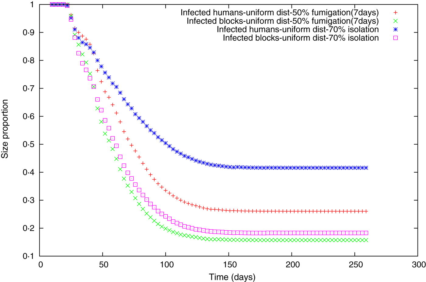
Fig. 4 [colour online]. Size of the biggest cluster for random uniform movement, in terms of number of infected humans for 50% fumigation (+), and 70% isolation (![]() ), or in terms of the number of blocks occupied for 50% fumigration (×) and 70% isolation (□).
), or in terms of the number of blocks occupied for 50% fumigration (×) and 70% isolation (□).
For both strategies we observed that the proportion of the biggest mass cluster is higher than the geometric one (Fig. 4), but the proportional difference between the curves of the biggest mass and geometric clusters is appreciably different between the two measures. This indicates that in the isolation case even though the final epidemic sizes might be similar, infected people are less dispersed compared to the fumigation case.
DISCUSSION
The present model represents a balance between the need to understand and quantify interventions and our current knowledge. In general, and this paper is not an exception, mathematical models allow the extrapolation and integration of knowledge, but this demands a hierarchical organization of the information in somewhat complete levels. Lack of knowledge at higher levels makes incorporation of details at lower levels irrelevant. In the present case, for example, it is known that A. aegypti activity is mostly diurnal with peaks at sunrise and sunset [Reference Yasuno and Tonn43] but introducing this knowledge would require a corresponding detail on the time-interval spent by humans at work, home and other places, and a detailed knowledge of the mosquito populations at each of these places, such information is not available and would be extremely difficult to obtain. Other matters like weather fluctuations that affect mosquito populations [Reference Romeo44] and heterogeneities in breeding sites and human population can be incorporated but need to be done on a particular basis and are expected to produce little change in the average behaviour captured by the current model. Thus incorporating them will result more in an illusion of realism than in any real improvement of the general analysis. Finally, under the pressures created by a dengue epidemic outbreak, knowledge of the immunological status of the population would be required to gauge the number of severe dengue cases that could overburden the health system. However, these facts have no dynamic effects except for the presence of a certain number of recovered/immune people. The case we have considered corresponds to a city like Buenos Aires, without any records of any relevant dengue epidemic. In other words, in our view, more accurate results can only be given for particular cases and not in general.
The first intervention measure analysed was the movement restriction strategy. It was found, rather unexpectedly, that this policy has little to no effect on the FSEs and on its probability compared to the no-measure scenario. In order to understand this result, we compared these two strategies, i.e. no measures and movement restriction. For this purpose we counted how many mosquitoes were infected by humans in each of the 5 days of the human VP, and also which of those were infected by humans at ‘home’ or at ‘work’. We also performed the same calculation taking into account only those mosquitoes that were infected in a block free of infected/or exposed mosquitoes (generation of new mosquito foci of infection). A focus is said to start at the ith day of viraemia, if infectious humans have failed to establish the mosquito foci by days j<i, while those which are bitten during the ith day of viraemia succeeded. The obtained results are shown in Table 7. Under the no-intervention strategy the total number of mosquitoes infected by humans at work between days 3 and 5 of infection was only about 12% of the total. However, this is a small percentage of the total. Moreover, when considering the case in which the restriction in movement is applied, it was found that this 12% is transferred to the infections produced at home between days 3 and 5 of human infection, ‘preserving’ in that way the total amount of infectious bites.
Table 7. Number (percentage) of mosquitoes infected during two particular simulations with Levy 2 human movement and similar FSE. The infected mosquitoes are classified by the viraemic day of the human from whom it acquired the virus and whether this human was at home or work at the time of infection

Top, No measures; bottom, movement restriction strategy.
Moreover, from our simulation (not shown in the Tables) in the no-measures scenario, the creation of new mosquito foci by humans at work between days 3 and 5 of infection is around 10% which we believe is small enough not to affect the evolution of the epidemic if removed by the application of the movement restriction strategy (there can not be new mosquito foci created at work between the times on which we restrict the human movement by definition). To check whether the inefficiency of the movement restriction strategy was due to low breeding site density (BS) used in the simulations or due to the distribution of time between work and home, we tried several other conditions and always observed the same behaviour.
By contrast, we found the isolation strategy to be quite effective. From Table 7 it can be seen that almost 70% of the total infective bites in the no-measures scenario were made on humans between days 3 and 5 of infection, which we are isolating if using the 3-day isolation strategy. We performed isolation strategies of 1, 2 or 3 days of human isolation during the infective period and observed that all the isolation strategies are highly effective not only by reducing the final epidemic size but also by reducing the probability of epidemics. This probability is obviously lowered because in the case of isolation strategies some of the five possible days for the index case to infect a mosquito are removed. As expected, both final size and probability are lower when the duration of human isolation is increased. It can also be seen that the median of the FSE and the probability P e are not linear with the duration or length of isolation because the model is highly nonlinear and the probabilities of infection for human–mosquito transmission are not uniform [Reference Nishiura and Halstead37].
Since in reality, isolation strategies cannot always be started from the very beginning of an epidemic outbreak we ran simulations of the 3-day isolation strategy for different days of delay from the appearance of the index case (Fig. 3). It can be seen that with delays from 0 to 14 days the probability of an epidemic grows but thereafter all consecutive delays have the same probability. Note that in the 0-day delay scenario we always isolate the last three infective days of the index case. In the case of ⩾14-day delays, whatever the length the exposition time of the index case, there is no possibility of isolation, so the probability of an epidemic outbreak will be the same as for the no-measure scenario.
We show that there are no differences between the empirical distribution functions for 14-day and 21-day isolation strategies. To explain this observation it should be noted that the EIP of the mosquitoes is fixed to 10 days, therefore we realize that if there is going to be any difference between these two delays it is because the first secondary infected human appears in the interval between 14 and 21 days. If we check all the possibilities with their probabilities we realize that this seldom happens and that is why these two cases are almost the same. These findings are important because they mean that there exists a window of time which is the same when we start the isolation strategy. However, if we extend the delay beyond a certain limit (e.g. 60 days), we see that the distribution gets closer to that without measures but still reduces the final epidemic size. For a 120-day delay (roughly at the peak of the epidemic) it can be seen that the measure is no longer effective.
As explained previously, it is expected that not all infected people are going to achieve isolation, either because they decide not to obey the strategy or because they do not know they are infected (subclinical cases with mild or no symptoms). We ran simulations with different efficiencies of isolation to study their impact on the evolution of the disease. As we have already noted the probability of epidemics decreases with the efficiency of the isolation (Table 3). The difference between the probability of epidemics under a no-measure strategy and the probability of epidemics under an isolation strategy with 100% efficiency (≃44% for the Levy 2 case) is due to the possibility of the index case being bitten during the last 3 days of the VP. If the efficiency were other than the maximum, it is straightforward to see that the probability of an epidemic would be
 $$\eqalign{P_{{\rm e}} = {\rm} P_{\rm no\,measures}*\!({\rm 1} - {\rm efficiency}) + P_{{\rm 100\%}}*\!{\rm efficiency}},$$
(the probability of the epidemic starting during those last 3 days is linear with the efficiency of isolation since it is decided at the start whether the index case is isolated or not for the whole simulation). If we check these probabilities (Table 3) taking into account the errors then it is fulfilled. It can also be seen that the mean of the FSEs decreases with isolation efficiency, but not linearly.
Interventions to control mosquito populations are perhaps the most common approach during dengue epidemics; we considered the case of fumigation. We observed that low-efficiency fumigations (efficiencies of 10% and 30%) are capable of reducing the FSEs but do not substantially decrease the probability of epidemics. Moreover, the use of low-efficiency fumigation interventions requires a high number of fumigations during the epidemic outbreak. By contrast, the model shows that high-efficiency fumigations are effective in reducing both the FSEs and the probability of epidemics, requiring a smaller number of insecticide applications. Nevertheless, compared to human isolation (Table 3), fumigation is less efficient at lowering the probability of epidemic outbreaks even when the final epidemics sizes are similar. We also performed simulations with 3-day intervals (not shown) which are, as expected, more efficient both in final size and total number of fumigations, but this shorter interval does not seem to affect the epidemic probability. This is to be expected because between the index case and the second infected human there can be only one fumigation regardless of the interval chosen.
The effectiveness of peridomestic insecticide spraying in reducing dengue transmission has not been conclusively demonstrated [Reference Ekpereonne41]. Therefore, we studied insecticide spraying in combination with human isolation strategies as a possible form to increase effectiveness in dealing with dengue outbreaks. Combined strategies performed with the model (Table 5) have the advantage of presenting low epidemic probabilities, because of the isolation, and low epidemic sizes even for low efficiencies both in isolation and in fumigation. Moreover, the required amounts of insecticide applications are lower compared to single measures of fumigation with same efficiency. It is also worth noting that the effect on the FSEs seems to be additive. We are able to compare the percentage of FSEs reached with each strategy, with regard to the case under no-intervention measures. For example, in the case of the Levy flight pattern (Table 5) for the 50% isolation strategy the percentage was 29%, for the 30% fumigation strategy it was 23%, when these values are multiplied the result is close to the 7% reached with the combined policy using the same efficiencies. In a way, the isolation effect seems to be independent of the fumigation effect.
We also studied the effect of subclinical cases during an epidemic outbreak and observed that the fumigation strategies were still effective in the reduction of the FSEs. However, in the worst scenario with a high proportion (90%) of subclinical cases, the P e almost reached the value under the no-intervention measure. For example, in the case of a uniform pattern during a fumigation strategy with an efficiency of 50% and with 90% of subclinical cases (Table 6), the P e rises to 0·78 and the FSE reaches a value of 62% of the FSE under the no-intervention measure. For the combined strategies the effect of the subclinical cases on the FSE and P e is similar, but in this case it is preferable to compare it with the isolation strategies and the combined strategies without subclinical cases. For example, in the case of a uniform pattern with an isolation efficiency of 50%, a fumigation efficiency of 50% and with 90% of subclinical cases, the P e reaches 0·55, almost the P e of the 50% isolation measure (0·56) and the FSE reaches a value of 14·5%, which is between the values reached with the combined strategy (3·2%) and the isolation strategy (23·1%) without subclinical cases.
Following the spatial analysis performed in our previous work [Reference Barmak29], several spatial analyses were conducted in order to study the differences between each of the individual strategies. Between pairs of strategies leading to similar FSEs we computed three analyses: the probability of finding at least one infected human at distance R from the index case, the cluster size distributions of infected people at different moments of the outbreak, and the size of the biggest cluster of infected people in relation to the size of all the aggregated infected clusters at different moments of the evolution of the epidemic. We failed to find any substantial differences between pairs of strategies for the two first analyses. Nevertheless, regarding the third spatial analysis (Fig. 4), we observed that the proportion of the biggest mass cluster is higher than the geometric cluster; this occurs because during the simulation several new human foci are created when the temperature is decreasing (autumn season) and these foci do not reach a size as big as the earlier clusters, principally generated during the summer season (in terms of number of infected people). So, there are several blocks with small numbers of infected humans compared to the biggest cluster which is often the cluster where the index case is. We also observed that the proportional difference between the curves of the biggest mass and geometric clusters is appreciably different between the two policies represented as an example in Figure 4, which indicates that under isolation even though the final epidemic sizes are similar, infected individuals are less dispersed during the isolation strategy compared to the fumigation case.
In conclusion, we have developed an improvement of a previously published model [Reference Barmak29], which couples simultaneously the dynamics of humans with those of mosquitoes, allowing the simulation of complex control strategies acting on humans (e.g. movement restriction, isolation strategies, etc.) and/or mosquitoes (e.g. insect spraying) depending on the evolution of an epidemic outbreak.
Regarding isolation strategies, we studied those with different efficiencies and different delays at the beginning of the measures and observed a peculiar dependence of the FSE distribution on the delay at the beginning of the isolation measures. There is a first window for which only the probability of an epidemic changes and the FSE distribution shape does not change, and a second window for which the FSE distribution changes but the P e does not. The first window ensures that in that time span only the P e will grow and the maximum number of total infected humans will be bounded by the maximum of the FSE distribution. The second window shows that from that time on, the P e will be the same but the FSE will depend on the delay at the beginning of the isolation measure. That means that isolation strategies could be implemented even if the outbreaks are not recognized from the outset, even up to 60 days after the arrival of the index case. In particular there is a window of about 1 week (between 14 and 21 days after the appearance of the index case) for which both FSE and P e are similar, which means that during this period it does not matter when we start the strategy.
We studied insecticide spraying strategies with different efficiencies and with different proportions of subclinical cases in the human population and observed that highly efficient fumigation strategies seem to be effective during an outbreak. Nevertheless, taking into account the controversial results of spatial spraying as a single control strategy, the development of insecticide resistance, the high costs of vector controls, the high proportion of subclinical cases, and finally, based on our simulation results, we suggest that carrying out combined strategies of fumigation and isolation during an epidemic outbreak represents a suitable strategy for the attenuation of epidemic outbreaks.
It should be noted that all results discussed are qualitatively similar regardless of the human mobility pattern used (random uniform and Levy 2).
APPENDIX A
Algorithmic description of the model
As we already described in the Methods section, 28 different subpopulations for the mosquito are considered. According to the biological stages of the mosquito and its disease status we considered three immature subpopulations: eggs E, larvae L and pupae P and 25 adult subpopulations: susceptible female adults not having laid eggs A1, susceptible flyers F s, exposed flyers during the 10 different days of the EIP, F e(k) with 1⩽k⩽10, infectious flyers F i, and female adults having laid eggs in the three disease compartments: susceptible A2s, exposed A2e(k) with 1⩽k⩽10 and infectious A2i.
Eggs, larvae, pupae and non-parus adults, A1, are considered susceptible. After a blood meal A1 becomes a flyer, susceptible F s or exposed F e(1) in the first day of the EIP, depending on the disease status of the host bitten.
The evolution of the 28 subpopulations is affected by 68 different possible events (see Table 1 and Fig. 1), and is modelled by a state-dependent Poisson process [Reference Ethier and Kurtz38, Reference Andersson and Britton39] where the probability of the state [E, L, P, A1, A2s, A2e(1), …, A2e(10), A2i, F s, F e(1), …, F e(10), F i] evolves in time following a Kolmogorov forward equation which can be constructed directly from the information presented in Table 1.
The numerical implementation of the stochastic model is performed with a 2-h time step using a Poisson approximation [Reference Solari and Natiello40]. In each 2-h subunit the model calculates for each block all mosquito subpopulations and events presented in Table 1. The vector contagion event is not calculated in the same way since vector contagion requires the interaction between vectors and hosts. The description of vector and human contagion dynamics is presented in an algorithmic way as follows:
-
(1) Start of the 2-h loop.
-
(2) Calculation of the number of each kind of event (Table 1) which is approximated by independent Poisson processes [Reference Otero and Solari24, Reference Otero, Schweigmann and Solari35, Reference Otero, Solari and Schweigmann36, Reference Solari and Natiello40].
-
(3) Random distribution of the bites performed by A1 and A2s between all humans (events 8 and 21, respectively), and then computation of the number of these bites on humans on each day (j) of their infectious state, B I (j).
-
(4) Calculation of how many mosquitoes were actually exposed, M NE, using binomial distributions for the B I (j)'s with p hm(j) probabilities (the probability of human–mosquito contagion is dependent on the human stage-day of the VP).
-
(5) Update of the state of F e(1) subpopulations: F e(1) = F e(1) + M NE.
-
(6) Random distribution of the bites performed by A2i (event 32) between all humans and construction of a table of bitten individuals.
-
(7) Update of the human population and the rest of the mosquito subpopulations.
-
(8) Update of the exposed and infectious mosquito subpopulations if the program is at the 12th time subunit (end of the day):
 $$F_{\rm e} (k + {\rm 1}){\rm} = {\rm} F_{\rm e} (k)\quad {\rm if}\quad {\rm 1} \les k \les {\rm 9},$$
$$A{\rm 2}_{\rm e} (k + {\rm 1}){\rm} = {\rm} A{\rm 2}_{\rm e} (k)\quad {\rm if}\quad {\rm 1} \les k \les {\rm 9},$$
$$F_{\rm i} {\rm} = {\rm} F_{\rm i} {\rm} + {\rm} F_{\rm e} (10),$$
$$A{\rm 2}_{\rm i} {\rm} = {\rm} A{\rm 2}_{\rm i} + {\rm} A{\rm 2}_{\rm e} ({\rm 1}0),$$
$$F_{\rm e} ({\rm 1}){\rm} = {\rm} 0,$$
$$A{\rm 2}_{\rm e} ({\rm 1}){\rm} = {\rm} 0.$$
$$F_{\rm e} (k + {\rm 1}){\rm} = {\rm} F_{\rm e} (k)\quad {\rm if}\quad {\rm 1} \les k \les {\rm 9},$$
$$A{\rm 2}_{\rm e} (k + {\rm 1}){\rm} = {\rm} A{\rm 2}_{\rm e} (k)\quad {\rm if}\quad {\rm 1} \les k \les {\rm 9},$$
$$F_{\rm i} {\rm} = {\rm} F_{\rm i} {\rm} + {\rm} F_{\rm e} (10),$$
$$A{\rm 2}_{\rm i} {\rm} = {\rm} A{\rm 2}_{\rm i} + {\rm} A{\rm 2}_{\rm e} ({\rm 1}0),$$
$$F_{\rm e} ({\rm 1}){\rm} = {\rm} 0,$$
$$A{\rm 2}_{\rm e} ({\rm 1}){\rm} = {\rm} 0.$$
-
(9) End of the 2-h loop.


Repetition of the loop again.
APPENDIX B
Model parameters
Developmental rate coefficients
The developmental rates that correspond to egg hatching, pupation, adult emergence and the gonotrophic cycles were evaluated using the results of the thermodynamic model developed by Sharp & DeMichele [Reference Sharpe and DeMichele45] and simplified by Schoofield et al. [Reference Schoofield, Sharpe and Magnuson46]. In this model the maturation process is controlled by one enzyme which is active in a given temperature range and is deactivated only at high temperatures. The development is stochastic in nature and is controlled by a Poisson process with rate R D(T), which takes the form
 $${\eqalign{R_{\rm D} (T) = R_{\rm D} (298K) \times\displaystyle{{(T/298K)^*{\rm exp}\; ((\Delta H_{\rm A} /R)(1/298K - 1/T))} \over {1 + {\rm exp}\; (\Delta H_{\rm H} /R)(1/T_{1/2} - 1/T))}}}},$$
where T is the absolute temperature, ΔH A and ΔH H are enthalpies characteristic of the organism, R is the universal gas constant, and T ½ is the temperature when half of the enzyme is deactivated because of high temperatures.
Table 2 presents the values of the different coefficients involved in the events: egg hatching, pupation, adult emergence and gonotrophic cycles. The values are taken from [Reference Focks47] and are discussed in [Reference Otero, Solari and Schweigmann36].
Mortality coefficients
Egg mortality
The mortality coefficient of eggs is me = 0·011/day, which is independent of temperature in the range 278 K⩽T⩽303 K [Reference Trpis48].
Larval mortality
The natural regulation of Aedes aegypti populations is due to intra-specific competition for food and other resources in the larval stage. This regulation was incorporated into the model as a density-dependent transition probability which introduces the necessary nonlinearities that prevent a Malthusian growth of the population. This effect was incorporated as a nonlinear correction to the temperature-dependent larval mortality. Larval mortality can then be written as: ml*L+αL*(L –1) where the value of α can be further decomposed as α=α 0 /BS with α 0 being associated with the carrying capacity of one (standardized) breeding site and BS being the density of breeding sites in the grid [Reference Otero, Schweigmann and Solari35, Reference Otero, Solari and Schweigmann36].
The value of α 0, associated with the carrying capacity of a single breeding site, is α 0 = 1·5 [Reference Otero, Solari and Schweigmann36]. The temperature-dependent larval death coefficient is approximated by ml = 0·01 + 0·9725 exp(–(T–278)/2·7035) and is valid in the range 278 K⩽T⩽303 K [Reference Horsfall49–Reference Rueda51].
Pupal mortality
The intrinsic mortality of a pupa has been considered as mp = 0·01 + 0·9725 exp(−(T−278)/2·7035) [Reference Horsfall49–Reference Rueda51]. Besides the daily mortality in the pupal stage, there is an additional mortality associated with the emergence of the adults. We consider a mortality of 17% of the pupae at this event, which is added to the mortality rate of pupae, hence the emergence factor is ef = 0·83 [Reference Southwood52].
Adult mortality
Adult mortality coefficient is ma = 0·091/day, which is considered independent of temperature in the range 278 K⩽T⩽303 K [Reference Horsfall49, Reference Christophers53, Reference Fay54].
Oviposition coefficient
Females lay a number of eggs that is roughly proportional to their body weight (46·5 eggs/mg) [Reference Bar-Zeev55, Reference Nayar and Sauerman56]. Considering the mean weight of a 3-day-old female is 1·35 mg [Reference Christophers53] we estimate the average number of eggs laid in one oviposition as 63.
The oviposition coefficient ovr depends on breeding site density BS and is defined as:
 $$ovr = \left\{ {\matrix{ {\theta /tdep} & {\;{\rm if}\;} & {BS \les 150} \cr {1/tdep} & {\;{\rm if}\;} & {BS \gt 150}}} \right.$$
where θ was chosen as θ=BS/150, a linear function of the density of breeding sites [Reference Otero, Schweigmann and Solari35] and tdep = 0·229 days [Reference Christophers53].
Dispersal coefficient
The general rate of the dispersal event is given by: disp*F, where disp is the dispersal coefficient and disp = 0·664. The implementation of flyer dispersal has been described elsewhere [Reference Otero, Schweigmann and Solari35].
ACKNOWLEDGEMENTS
We acknowledge the support of the University of Buenos Aires (Argentina) through grants 20020110100205 and 20020100100734.
DECLARATION OF INTEREST
None.


