


Media summary: Fitness-maximizers employ pessimistic probability weighting for decisions under risk.
1. Introduction
A herder in in the arid north of Kenya has to make decisions about the composition of his herd (Mace & Houston, Reference Mace and Houston1989; Mace, Reference Mace1990, Reference Mace1993). Should he restrict his herd to small, high-productivity goats or, when he gets enough goats, should he trade them for larger, slower-breeding camels? The growth rate of goat herds, even accounting for their increased susceptibility to high mortality during drought years, is three times that of camels and the expected energetic payoff to keeping goats – more precisely, the instantaneous rate at which wealth accumulates – is therefore substantially higher than a mixed herd of goats and camels. However, pastoralists in the region favour mixed herds and will even increase the fraction of camels dramatically above a critical wealth threshold (Mace &Houston, Reference Mace and Houston1989; Mace, Reference Mace1990). Are these herders engaging in irrational economic decision making by under-valuing the payoff of an all-goat herd? While the expected return is lower for a mixed herd of predominantly camels, households pursuing this strategy have a much higher probability of long-term persistence, nearly 70%, compared with a 0.4% probability of persistence for the goats-only strategy. Why is this so?
In part, mixed herding diversifies risk. More importantly, however, the growth of these herds, like any biological growth process, is multiplicative and the rate of increase is stochastic. Furthermore, the herder faces more than just a decision about long-term wealth accumulation, a well-studied topic in finance (e.g. Karatzas & Shreve, Reference Karatzas and Shreve1998) and economics (e.g. Peters & Gell-Mann, Reference Peters and Gell-Mann2016). Rather, herd products and income from the herd provide each household's primary yearly consumption, and consequently there are two processes that matter to the herder: herd growth and household consumption. We might better interpret the herder's decision as not about herd management, per se, but rather about household consumption through time, for which herd dynamics can lead to very uneven yearly consumption that cannot be fully accounted for by available smoothing mechanisms.
Like growth of the herd, household survival can be thought of as a stochastic gamble in which the survival probability is a function of household consumption. For such a multiplicative process, a severe shortfall in any time period that leads to a low survival probability can never be compensated for by high survival in other time periods (even a large number of other time periods). A virtually identical perspective arises when considering the evolutionary fitness of individuals because, as we will describe and formalize, fitness is determined by stochastic, multiplicative processes; most obviously, individual survival through time is a component of fitness, and like household survival, individual survival is a binary outcome variable with differing probabilities for each time period. In this article, we explore what this means for the evolution of organisms’ decision making.
Our challenge is to account for how selection might construct a decision-making system that is responsive to fitness-relevant decisions in real, variable environments. The first core contribution of this paper is our suggestion of a hierarchical framework for evolutionary decision making that arises naturally from Mayr's proximate/ultimate distinction (Mayr, Reference Mayr1961). We then employ the logic of an evolutionary principal–agent problem, an idea we adopt from Binmore (Reference Binmore1994), to link proximate and ultimate ends. This framework reflects the limitations natural selection faces in imparting fitness-optimizing behaviours to organisms. Other authors have suggested that natural selection addresses these limitations by imparting proximate preferences to agents. However, we add that natural selection may have separately, or in tandem, influenced more than one component of human decision making. Much like the utility function in expected utility theory, proximate currencies can be used to map the consequences of specific decisions onto evolutionarily salient proximate variables such as fertility and survival. The hierarchical model we propose possesses proximate value functions that map consumption onto proximate variables, while probability weighting fixes a mismatch that arises from the enforced inability of these value functions to respond to time-dependent environmental uncertainty.
Our second core contribution arises from applying this framework and understanding the consequences of selection for both the value functions mapping consumption to proximate currencies and the probability weighting that then links these to fitness. It has long been recognized in evolutionary biology that stochastic fluctuations in single-period growth rates lower the long-term growth rate below what would be achieved from deterministic growth at the mean rate each period (Haldane & Jayakar, Reference Haldane and Jayakar1963; Lewontin & Cohen, Reference Lewontin and Cohen1969; Tuljapurkar, Reference Tuljapurkar1982). In our hierarchical framework, we limit the role of value functions to only map consumption onto proximate outcomes such as age-specific fertility and mortality (we do allow that the mapping itself can depend on environmental or social contexts). Hence, they can play no role in addressing the long-term lowering of fitness exacted by environmental stochasticity. This is where the probability weighting contributes to the model. The optimal level of weighting does depend on the exact universe the organism occupies, which sets the gambles the organism faces and how those gambles vary with time. We show that, regardless of these details, the optimal probability weighting involves pessimistic probability weighting. This result is of fundamental theoretical importance because it links evolutionary theory with important work in economics. Pessimistic probability weighting of unlikely, negative outcomes is a core aspect two of the most successful behavioural economic models, rank-dependent expected utility theory and cumulative prospect theory, both of which recover expected utility theory as a special case. We thus offer a grounded evolutionary explanation for one of the cornerstones of modern behavioural economics.
Because we anticipate a diverse readership for this article, we have provided substantial background material, especially in Sections 2 and 5. Section 2 summarizes pertinent economic ideas, notably expected utility theory and alternatives to it such as rank-dependent expected utility theory. Section 3 frames our hierarchical model with respect to recent literature on the evolution of economic preferences, describes the evolutionary principal–agent problem and summarizes our hierarchical model. Section 4 gives a high-level, verbal outline of our model. Section 5 describes the evolutionary component of our model, stochastic age-structured population models (the economic model, rank-dependent expected utility theory, is described in Section 2). Section 6 brings together the preceding material to establish our core result on pessimism. Section 7 discusses our results.
2. Expected utility theory and its alternatives
Organisms, humans included, must make decisions about foraging, reproductive, social and political behaviours that have consequences for proximate outcomes such as satiety, income, wealth, happiness, sexual satisfaction and well-being. These decisions also have consequences for ultimate outcomes such as fitness and, consequently, there are strong expectations that selection acting on differential fitness will shape the decision-making system. The rational-choice tradition suggests that individuals make decisions that maximize some quantity typically denoted by the catch-all term ‘utility’. In the presence of variability in outcomes, the objective function for maximization is the expectation of utility. In particular, a set of possible payoffs (i.e. a ‘lottery’) ${\bf x} = [ {x_1\comma \;x_2\comma \;\ldots \comma \;x_n} ] ^{\rm T}$ with associated probabilities ${\bf p} = [ {p_1\comma \;p_2\comma \;\ldots \comma \;p_n} ] ^{\rm T}$
 is preferred to some other lottery ${\bf y} = [ {y_1\comma \;y_2\comma \;\ldots \comma \;y_n} ] ^{\rm T}$
 with probabilities ${\bf q} = [ {q_1\comma \;q_2\comma \;\ldots \comma \;q_n} ] ^{\rm T}$
 if some preference functional (Machina, Reference Machina1982) that associates payoffs with probabilities $V\lpar {{\bf x}\semicolon \;{\bf p}} \rpar$
 is greater than that associated with $V\lpar {{\bf y}\semicolon \;{\bf q}} \rpar$
 : $V\lpar {{\bf x}\semicolon \;{\bf p}} \rpar \gt V\lpar {{\bf y}\semicolon \;{\bf q}} \rpar$
 . Here and elsewhere vectors (bolded) are column vectors by default and T indicates a transpose. A preference functional thus contains two inputs: (1) a measure of the value of outcomes (i.e. utilities associated with outcomes); and (2) weights for these outcomes. In the absence of other information, a reasonable value function is linear in the probabilities and utilities of distinct outcomes,

This linear specification yields an expectation over utility and the theory that uses maximization of expected utility is known as expected utility theory (EUT). This theory was first formalized in its modern form by von Neumann and Morgenstern (Reference von Neumann and Morgenstern1947) and further axiomatized by Savage (Reference Savage1954). Expected utility, combined with exponential time discounting of delayed outcomes, represents the canonical economic model of decision making (Samuelson, Reference Samuelson1937; von Neumann & Morgenstern, Reference von Neumann and Morgenstern1947; Machina, Reference Machina1982; Starmer, Reference Starmer2000; Frederick et al., Reference Frederick, Loewenstein and O'Donoghue2002). The EUT approach has been very fruitful for economics, political science and other behavioural sciences. Like many economic theories it is axiomatic and the fundamental axioms that underlie EUT (completeness, transitivity, continuity and independence) are sensible requirements that ensure that preferences are consistent (von Neumann & Morgenstern, Reference von Neumann and Morgenstern1947; Savage, Reference Savage1954). However, an enormous literature has developed showing that people violate the axioms underlying EUT in both experimental and naturalistic contexts. Some examples include the common consequence effect (Allais paradox), the common ratio effect (Allais, Reference Allais1953), ambiguity aversion (Ellsberg, Reference Ellsberg1961), preference reversals between gambles represented as bids vs. choices (Lichtenstein & Slovic, Reference Lichtenstein and Slovic1971), the incommensurability of risk-sensitive behaviour for high- vs. low-stakes gambles (Rabin, Reference Rabin2000), overconfidence (Heller, Reference Heller2014) and abundant evidence that framing and reference points induce departures from canonically predicted behaviour (Kahneman & Tversky, Reference Kahneman and Tversky1979; Tversky & Kahneman, Reference Tversky and Kahneman1992; Loewenstein & Prelec, Reference Loewenstein and Prelec1992). Violations of the stationarity of time preferences, another canonical assumption although not the focus of this article, include the common difference effect and the absolute magnitude effect (Loewenstein & Prelec, Reference Loewenstein and Prelec1992; Frederick et al., Reference Frederick, Loewenstein and O'Donoghue2002).
One consequence of these empirical observations is that they spurred theorists to develop new choice models that could accommodate the empirical findings. Starmer (Reference Starmer2000) divides these efforts into conventional and non-conventional. Regarding the conventional strategy, Starmer (Reference Starmer2000, p. 338) writes, ‘The general spirit … is to seek “well behaved” theories of preferences consistent with observed violations of independence’. In this spirit, Starmer defines conventional theories as those that maintain the completeness, transitivity and continuity axioms, but rather than maintaining the independence axiom insist on monotonicity, ‘the property that stochastically dominating prospects are preferred to prospects which they dominate’ (Starmer, Reference Starmer2000, p. 335). First-order stochastic dominance occurs when the cumulative distribution function (or cumulative mass function for a discrete distribution) of a gamble is at least equal to that of another gamble over its entire domain (Quiggin, Reference Quiggin1993, p. 77). It is common to require the cumulative distribution function to be strictly greater than that of the other gamble on at least part of its domain (Wakker, Reference Wakker2010, p. 65).
The reason Starmer uses independence as the criterion to distinguish conventional from non-conventional theories is that its violation was (and almost certainly is) seen as the primary challenge to EUT arising from behavioural economics experiments. The independence axiom asserts that adding a common outcome to two prospects should not change the preference ordering of the prospects. Perhaps the most notable behavioural anomaly is the Allais paradox (Mongin, Reference Mongin2019, for a recent review), or common consequence effect, which uncovers a violation of the independence assumption. Quiggin (Reference Quiggin1993, p. 30) writes: ‘The Allais problem is the pons asinorum of theories of choice under uncertainty. Almost all of the many authors who have introduced new models of choice under uncertainty in the last 10 years [i.e. alternatives to expected utility theory] have included a demonstration that the model is consistent with the behaviour revealed in this problem’.
Machina (Reference Machina1981, Reference Machina1987) noted there is nothing inevitable about expected utility serving as the objective function for preference ordering and suggested that nonlinear functions mapping proximate values and probabilities might account for these types of systematic departures from the predictions of EUT. An important class of non-linear models that can accommodate the Allais paradox does so via subjective probability weights. In the simplest formulation of probability weighting, the decision weights are a direct function of the probability of each individual outcome,

where ${\cal W}$ is the weighting function and p i is the probability of outcome i. Preson and Baratta (Reference Preson and Baratta1948) may have been the first to suggest the use of subjective probability weights in this way. They showed that when individuals could competitively bid on lotteries with uncertain outcomes they systematically over-weighted low probabilities (up to about p = 0.1) and under-weighted high probabilities. This straightforward method of probability weighting was adopted in the original formulation of prospect theory (PT; Kahneman & Tversky, Reference Kahneman and Tversky1979), an early, heuristic-based alternative to EUT that gained widespread attention. However, it was quickly pointed out that PT and other theories that simplistically implement probability weighting violate monotonicity (Wakker, Reference Wakker2010, p. 153). An ad hoc fix of the PT violation of stochastic dominance was incorporated via an editing process that occurred before the probability weighting occurred. In addition to lacking parsimony, this editing process can induce intransitivity in pairwise choices (Quiggin, Reference Quiggin1982). The appeal of PT was its selective incorporation of the more desirable features of EUT, while nevertheless rejecting the independence axiom, so that the Allais paradox and other behavioural violations could be accommodated, but a model that leads to the favouring of stochastically-dominated choices or intransitivity was clearly unacceptable.
The publication and response to PT spurred work to develop alternatives, including axiomatic, conventional theories (sensu Starmer) that maintained EUT's less controversial axioms (completeness, transitivity, and continuity) while simultaneously avoiding the violation of stochastic dominance exhibited by PT in its unedited form. The culmination of this work was the simultaneous and independent discovery of RDEUT by at least three scholars (Quiggin, Reference Quiggin1982; Schmeidler, Reference Schmeidler1989; Yaari, Reference Yaari1987). RDEUT avoids violations of monotonicity by re-weighting probabilities in a quite specific manner. Assume that the probabilities of some prospect are sorted from most desirable to least desirable according to the values of their corresponding outcomes (x 1 ≥ x 2 ≥ x 3 ≥ ⋅ ⋅ ⋅ ). Next, define the cumulative probability, or rank (Wakker, Reference Wakker2010), as

where θ i is the probability of receiving an outcome that is as good as or better than i. The probability weighting on outcome i is given by

where w is the weighting function defined on ranks and we assume that θ 0 = 0. In equation (4), w is used rather than ${\cal W}$ to emphasize that w is defined on probability ranks, whereas ${\cal W}$
 is defined on probabilities; w maps the interval [0, 1] onto itself, must be an increasing function of θ, and must satisfy w(0) = 0 and w(1) = 1. The rank-dependent expected utility is

Figure 1 plots three different probability weighting functions. The middle curve is a standard form that exhibits two suggested biases in the psychophysics of probability distortions: likelihood sensitivity and pessimism (Gonzalez and Wu, Reference Gonzalez and Wu1999; Wakker, Reference Wakker2010). Likelihood sensitivity occurs because differences near the endpoints of the probability scale (0 and 1) loom larger than differences in the interior of the interval. Conversely, differences in the middle of the scale loom smaller, so that the difference between 0 and 1% is psychologically much more salient than the difference between 60 and 61%. To account for diminished likelihood sensitivity for intermediate probabilities, the probability weighting function must have an inverse-S shape so that the centre is more flat than the endpoints.

Figure 1. Probability weighting functions for the RDEUT model. The top curve exhibits optimism over its entire domain. The bottom curve exhibits pessimism. The middle curve is a standard curve adopted in much of the recent literature; it combines pessimism with likelihood sensitivity.
Pessimism involves the under-weighting of desirable outcomes relative to their probability of occurrence, and leads to an overall lowering of the weighting function. Two types of pessimism can be defined relative to the probability weighting function, w(θ): regular pessimism and strong pessimism (Quiggin, Reference Quiggin1993). Regular pessimism (or simply pessimism) occurs where w is below the identity line w = θ, whereas optimism occurs where w is above the identity line. Strong pessimism occurs where w is convex (second derivative greater than zero), whereas strong optimism occurs where w is concave (second derivative less than zero). For many functional forms of w, regular pessimism and strong pessimism occur on the same or nearly the same intervals (and similarly for optimism).
RDEUT accounts for the Allais paradox through pessimistic probability weighting. Segal (Reference Segal1987), for example, has formulated a general statement of the Allais paradox using arbitrary payoffs and non-discrete probability distributions, and shown that RDEUT with a probability weighting function w exhibiting strong pessimism on its entire domain (i.e. the unit interval) can accommodate any and all formulations of the generalized Allais paradox. However, only a subset of the generalized formulations are encountered in daily life or economic choice experiments, so less restrictive probability weighting functions can accommodate the empirically relevant cases, although some pessimism is still a necessary element. For example, as already discussed, pessimism is one of the two primary components of the standard probability weighting curve (the other being likelihood sensitivity), which exhibits pessimism over only part of its domai n. Consequently, we utilize regular pessimism as opposed to strong pessimism as the relevant definition of pessimism. A crucial result proven by Quiggin (Reference Quiggin1993, chapter 6) follows from this assumption:
Theorem 1. If an RDEUT decision maker (agent) possesses a function u(⋅) that is increasing and concave, the following are equivalent,
(i) the agent exhibits regular pessimism, w(θ) ≤ θ.
(ii) the agent ascribes a lower value to the RDEUT than the EUT valuation, V (RDT) ≤ V (EUT).
When it was realized that RDEUT avoided violations of stochastic dominance and could accommodate the Allais paradox, PT was reformulated to include RDEUT, becoming cumulative prospect theory (CPT; Tversky & Kahneman, Reference Tversky and Kahneman1992). Consequently, RDEUT, either in its own right or as a component of CPT, is one of the most important components of contemporary work to generalize EUT (Starmer, Reference Starmer2000; Wakker, Reference Wakker2010).
Having summarized some of the pertinent economic ideas and models, we can now to turn to the central focus of the article. What mechanistic or functional basis might nonlinear preference functionals have? A reasonable working hypothesis is that their origins are found in evolutionary history. Indeed, there is a thread of evolutionary logic that runs through parts of the behavioural-economic literature. For example, an interpretation of Kahneman & Tversky's dual-process model, as articulated by Kahneman (Reference Kahneman2003, p. 697), suggests that ‘intuitive judgments occupy a position – perhaps corresponding to evolutionary history – between the automatic operations of perception and the deliberate operations of reasoning’. Various well-known decision biases – particularly loss-aversion – have been interpreted in light of evolutionary success (Haselton & Nettle, Reference Haselton and Nettle2006; McDermott et al., Reference McDermott, Fowler and Smirnov2008). Aside from this, there is a small but growing literature, mostly within economics, that seeks to model the evolution of human economic preferences (Rogers, Reference Rogers1994; Robson, Reference Robson1996; Robson & Samuelson, Reference Robson and Samuelson2009).
3. Natural selection, preferences and the evolutionary principal–agent problem
We are interested in economic decisions in the broadest sense. At the basic level, organisms are making decisions over what can be thought of as different lotteries. For example, should a herder focus on one animal or create a mixed herd? Should a forager hunt for sand monitor lizards or hill kangaroo (Jones et al., Reference Jones, Bliege Bird and Bird2013)? Should a peasant farmer intensify cultivation of a nearby garden plot or spread effort across two geographically distinct plots (Norman, Reference Norman1974)? Should a woman wean her infant and have another baby or continue nursing and delay reproduction (Hobcraft et al., Reference Hobcraft, MacDonald and Rutstein1983; Jones and Bliege Bird, Reference Jones and Bliege Bird2014)? Should an individual buy or rent a home (Shelton, Reference Shelton1968). In these examples, each lottery yields different payoffs probabilistically. All of these examples could have a clear impact on fitness, but it is extremely unlikely that any conscious fitness-maximization goal plays significantly into any of the decision makers’ choices. Instead, their decisions are shaped by preferences over a variety of proximate currencies like hunger/satiety, feelings of security or feelings of love and responsibility for children. Samuelson and Swinkles (Reference Samuelson and Swinkels2006) raise the important question, given the evolutionary mandate to successfully leave descendants, why do people have preferences for anything but fitness?
Why have preferences for proximate quantities?
In the substantial literature that addresses the question of why people have preferences for proximate currencies rather than fitness itself (Rogers, Reference Rogers1994; Binmore, Reference Binmore1994; Robson & Samuelson, Reference Robson, Samuelson, Benhabib, Bisin and Jackson2011; Glimcher, Reference Glimcher, Wilson and Kirman2016), three inter-related factors loom largest. First, natural selection operates on timescales that are longer than the lifespans of the organisms whose behaviour it shapes and, furthermore, selection is a stochastic, undirected process. Second, organisms regularly encounter novel situations for which natural selection is unable to directly specify behaviours. Third, the types of solutions that might emerge via natural selection to address the first two factors are constrained by trade-offs imposed by the cost of gathering and processing information. These observations can be accommodated within a single analytic framework by utilizing the economic concept of the principal–agent problem (Binmore, Reference Binmore1994), which will allow us to address the question of why organisms have preferences defined over proximate currencies, rather than the ultimate currency of fitness.
Consider a principal that possesses certain goals that it is unable to achieve unless it acts through agents over which it has only indirect control (Binmore, Reference Binmore1994). Natural selection is the ultimate arbiter of which biological entities remain and increase in a population. While the process of natural selection lacks agency, it is nonetheless useful to consider the outcomes of selection as having been designed (Williams, Reference Williams1966). It is in this sense that natural selection can be thought of as a principal with a goal of maximization of fitness. However, there are clear limitations in the ability of selection to achieve a solution, as enumerated above. Owing to the obvious lack of direct control, selection shapes cognitive mechanisms which are, on the whole, consistent with fitness maximization. As noted by Binmore (Reference Binmore1994), these collective proximate cognitive mechanisms can be thought of as the agent in the evolutionary principal–agent problem, wherein the principal (selection) ‘seeks to design an incentive scheme that minimizes the distortions resulting from having to delegate to the agents’ (Binmore, Reference Binmore1994, p. 151). The extent to which selection minimizes these distortions for a given organism in a given setting depends on the structure and strengths of the constraints it faces. A virtually identical perspective underlies the so-called ‘indirect approach’, in which the utility function is defined on proximate goods or outcomes, and the utility function in turn determines the success of an organism (Güth & Yaari, Reference Güth, Yaari and Witt1992; Güth, Reference Güth1995; Dekel et al., Reference Dekel, Ely and Yilankaya2007).
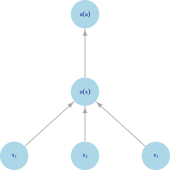
Figure 2 encapsulates the conceptual model that emerges from the principal–agent framework. At the bottom level, an individual is choosing between lotteries that influence the outcomes ${\bf x}_{\bf 1}\comma \;{\bf x}_{\bf 2}\comma \;\ldots$ . The outcomes of these lotteries contribute to utilities, u j, at the next level. These lotteries can be thought of either as motivational systems such as satiety, sexual gratification or happiness (akin to the classical notion of utility) or as proximate determinants of fitness such as infant survival or total fertility. What links these two different notions of ‘utility’ is that they work on a timescale where the organism can use feedback from outcomes to change its preferences and therefore decision making. These proximal utilities then contribute ultimately to fitness.
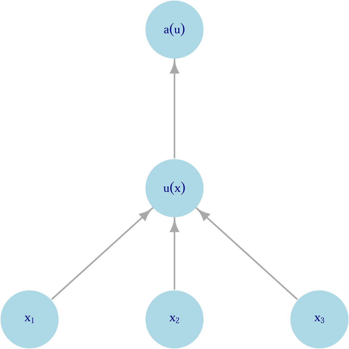
Figure 2. Hierarchical model of decision making as a principal–agent problem. Input variables (xi) contribute to intermediate utility (u(x)), which itself contributes to fitness (a(u)).
4. Model outline
The preceding section describes a conceptual framework for understanding the evolution of economic preferences. The main conclusion is that the evolutionary principal–agent problem implies the existence of proximate decision-making mechanisms within a hierarchical framework. In this section, we describe how to implement a formal model in accordance with this conceptual framework. In so doing, we provide a high-level summary of the actual model described below upon which our results and conclusions are based. Three elements are needed to apply the conceptual framework encapsulated by Figure 2: (1) an evolutionary model that defines how fitness depends on some determinants of fitness; (2) an economic model of decision making; and (3) a mechanism to link the evolutionary and economic models and thus provide novel predictions or insight into behaviour.
Evolutionary model
The evolutionary formalism we use is stochastic age-structured life history theory as described by Tuljapurkar (Reference Tuljapurkar1982). We assume a randomly mating, diploid population. Different phenotypes make different consumption decisions when faced with risk and environmental uncertainty. These differing consumption streams lead to different realizations of age-specific survival and fertility and thus to different growth profiles for the phenotypes. Tuljapurkar (Reference Tuljapurkar1982) shows that the rate of exponential growth (logarithm of the growth rate) of a phenotype, a, governs invade-ability (formalized below). In terms of Figure 2, the rate of exponential growth is the measure of fitness whereas age-specific survival and fertility – which change through time – are the determinants of fitness. The core result is equation (13), and readers already familiar with this result could skip the other material in the section.
Economic model
The economic formalism we use is RDEUT, which is summarized above in Section 2. The key result is Theorem 1.
Linking the models
To link the models, we assume that the determinants of fitness in the evolutionary model (age-specific survival and fertility) can be associated with the utility function in EUT. That is, at least to first order, an organism makes proximate decisions based on the expected values of the determinants of fitness. Other assumptions can be made to link the models, but we consider this an eminently sensible assumption to make given the limitations implied by the evolutionary principal–agent problem. It seems much easier for an organism to reason about the mean number of offspring a given strategy will yield (perhaps with a time discount factor applied on the timing of reproduction) than for an organism to reason about the ultimate fitness consequences of a given strategy.
However, we will show that averaging survival or fertility is systematically ‘wrong’ – i.e. leads to lower fitness – when stochastic uncertainty in achieved outcomes is accounted for. Specifically, the true fitness of a strategy that involves stochastic uncertainty is lower than that implied by the corresponding mean strategy that accounts for only mean survival and fertility. This is precisely the condition for pessimism in RDEUT and implies that an organism can ‘correct’ its expected utility bias by re-weighting the probabilities of a gamble as in RDEUT.
5. Stochastic, age-structured population matrices
To model the population dynamics and genetics, we utilize the formalism described by Tuljapurkar (Reference Tuljapurkar1982). We assume a diploid locus with alleles ${\cal A}^{\lpar m \rpar }$ (m = 1, 2, 3, …), random mating and a fixed sex-ratio, and ignore sex-differences. The genotypes ${\cal A}^{\lpar m \rpar }{\cal A}^{\lpar n \rpar }$
 code behavioural strategies that interact with the environment to determine an individual's life-history traits in each time period. Tuljapurkar (Reference Tuljapurkar1982) derives two essential results. First, he shows that the rate of exponential growth of ${\cal A}^{\lpar m \rpar }{\cal A}^{\lpar n \rpar }$
 governs invade-ability. That is, a population of homozygotes with allele ${\cal A}^{\lpar 1 \rpar }$
 is resistant to invasion by allele ${\cal A}^{\lpar 2 \rpar }$
 if a (11) > a (12), where a (mn) is the rate of exponential growth achieved by genotype ${\cal A}^{\lpar m \rpar }{\cal A}^{\lpar n \rpar }$
 . Second, Tuljapurkar provides an analytical formula for a when the variance in life history traits is small. The fundamental tool on which these results rely is the Leslie matrix; we introduce the Leslie matrix in the next section, then describe how stochastic uncertainty can be added.
Life history traits
Consider an age-structured population where each age class j accounts for individuals between y j = j Δy and y j+1 = (j + 1) Δy years of age. The key demographic traits that govern the population's dynamics are the age-specific fertility, F j, and the age-specific survival probabilities, P j. F j is the mean number of offspring that an individual in age class j contributes to the juvenile age class (j = 1) going from time t n to time t n+1 = t n + Δy, where n indexes time steps. P j is the probability that an individual will survive from age class j to age class j + 1. The Leslie matrix, ${\bf A}$ , has the age-specific fertilities on the first row and the age-specific survivals on the sub-diagonal,

where M is the number of age classes. The Leslie matrix projects the population vector ${\bf z}_n$ one time step into the future, ${\bf z}_{n + 1} = {\bf A}{\bf z}_n$
 . We assume that the Leslie matrix is irreducible and primitive (Caswell, Reference Caswell2001). Given these assumptions, there exists a unique dominant eigenvalue λ that is the per-period growth factor of the population. In the absence of stochastic fluctuations of the Leslie matrix elements, a = log λ (stochasticity is considered below). Hence, a population of homozygotes with genotypes ${\cal A}^{\lpar 1 \rpar }{\cal A}^{\lpar 1 \rpar }$
 is resistant to invasion by allele ${\cal A}^{\lpar 2 \rpar }$
 if λ (11) > λ (12). Associated with λ are the dominant left and right eigenvectors of ${\bf A}$
 , which we represent by v and ω, respectively. v is the vector of age-specific reproductive values and ω is the stable age distribution vector.
Stochastic uncertainty
We now account for stochastic uncertainty in the Leslie matrix elements. The crucial idea is that the Leslie matrix is not fixed from one time step to another, but instead depends on the changing state of the world. Following Tuljapurkar (Reference Tuljapurkar1982), consider an environmental sequence ${\cal E}$ with an associated sequence of Leslie matrices ${\bf A}_1\comma \;{\bf A}_2\comma \;\ldots \comma \;{\bf A}_n$
 . Let
. Let

represent the product matrix which governs population growth to time period n, and let λ n, ωn, and vn represent, respectively, the dominant eigenvalue, corresponding right eigenvector and corresponding left eigenvector of $^n {\bf Y}^1$ . Let $\tilde{\lambda }$
 , $\tilde{{\bi \omega }}$
 , and $\tilde{{\bi v}}$
 represent the corresponding quantities for the mean Leslie matrix. Without loss of generality, we assume that ωn and vn are normalized to 1. Weak ergodicity guarantees certain results. First, it guarantees that

Second, it guarantees the convergence of age structure to a stable age structure for any non-negative and non-zero starting vector ${\bf z}_0$ . To formalize this, let

be the normalized age structure at time period n, where the normalization is $\vert y \vert = \mathop {\mathop \sum \nolimits}\limits_k y_k$ . Then

An analogous result holds for ${\bi v}_n^{\prime}$ with left multiplication. The rate of exponential growth is

where ζ is an arbitrary initial age structure. Stochasticity lowers the rate of exponential growth compared with a non-stochastic reference Leslie matrix with the same mean life history traits. Effectively, this is because growth is a multiplicative process and the geometric mean is always less than the arithmetic mean (Lewontin & Cohen, Reference Lewontin and Cohen1969). Tuljapurkar (Reference Tuljapurkar1982) derives a useful ‘small noise approximation’ for a assuming small fluctuations of the Leslie matrix elements relative to the mean values,

where ${\bf C}$ is the covariance matrix of the mean covariance matrix $\tilde{{\bf A}}$
 , ⊗ is the Kronecker product, and the serial auto-correlation term in Tuljapurkar's approximation is not included. If only one Leslie matrix element is considered, equation (12) simplifies to

where $\sigma _{ij}^2$ is the stochastic variance associated with matrix element A ij. Equation (13) is the key evolutionary result. Caswell (Reference Caswell2010) provides a formula for the partial derivatives of λ with respect to the matrix elements,

Accommodating the hierarchical framework
The elements of the Leslie matrix, A ij, are the determinants of fitness at the intermediate level of Figure 2 (in this section, we do not explicitly show the time dependence of these matrix elements). We assume that they depend on a valuable but limited resource that can be traded off between fertility and survival across an individual's life cycle. More precisely, we assume that each Leslie matrix element A ij is an increasing function of the consumption x ij allocated to it with a negative second derivative (the latter condition ensures that weak pessimism is equivalent to the RDEUT sum being less than or equal to the EUT sum (Quiggin, Reference Quiggin1993, chapter 6). x ij is at the bottom level of Figure 2. For the reasons outlined in Section 3, we limit the role of proximate preferences in our model to accounting for the functional dependence of the A ij on the x ij, including how these mappings may depend on social or ecological context. This leaves a fitness mismatch that cannot be accommodated by proximate preferences since environmental stochasticity, which lowers the time-averaged rate of exponential growth, is unaccounted for. In the next section, we show that accounting for the effect of environmental stochasticity using probability weights implies pessimistic probability weighting.
6. Pessimism
In this section, we show that organisms that face uncertainty – arising, e.g. from the interaction of environmental fluctuations interacting with strategic choices – will act as pessimistic decision makers sensu RDEUT. Let s index strategies an agent can choose and let k index distinct outcomes (for example, achieved survival or fertility in a given time period). The agent faces uncertainty in choosing the strategy since the state of the world is not known when the strategy is chosen, but the agent does know the probability $p_k^{\lpar s \rpar }$ that each outcome will occur given strategy s. For notational convenience, we assume the outcome variable is age-specific fertility in some age class. For outcome k, the achieved fertility is f k; we use a lower case f to distinguish this fertility from the age-specific fertilities of the Leslie matrix in equation 6. The mean fertility for strategy s is

Table 1 illustrates this model for a simple case with three possible strategies and five possible outcomes. What makes these three strategies interesting is that they offer the same expected utility (i.e. fertility) but, as we show next, different evolutionary fitnesses. In particular, strategy s = 1 offers the highest fitness because it has the lowest variance and strategy s = 3 offers the lowest fitness because it has the highest variance. The gambles we discuss in this section all depend implicitly on underlying consumption levels that determine fertility. However, the details of the dependence do not impact the results so for simplicity we choose not to explicitly show them. Let ${\bf A}$ represent a Leslie matrix in which all elements are fixed except for one stochastic fertility term, $A_{1j}^{\lpar s \rpar }$
 , which equals f k with probability $p_k^{\lpar s \rpar }$
 as described above and summarized in Table 1. In equation (13), the second term is always negative. The effect of stochastic uncertainty, therefore, is to reduce a if the mean Leslie matrix is held constant. That is, $\sigma _{ij} \lt \sigma _{ij}^{\prime}$
 implies $a\left({\left\langle {\bf A} \right\rangle \comma \;\sigma_{ij}} \right)\lt a\left({\left\langle {\bf A} \right\rangle \comma \;\sigma_{ij}^{\prime} } \right)$
 , and vice versa. Strategy s = 1 in Table 1 is preferred to s = 2 and s = 2 is preferred to s = 3 since variance increases from s = 1 to s = 3.
Table 1. Three strategies with the same expected utility (fertility) but different evolutionary fitnesses; s = 1 is preferred to s = 2 is preferred to s = 3 since variance increases from s = 1 to s = 3. The first five rows summarize the outcomes for each achieved fertility level, with the first column giving the index k, the second column the fertility for each outcome, f k, and the remaining columns the probabilities of each outcome given the chosen strategy s. The last two rows summarize, for each strategy s, the mean and standard deviation for fertility

The stage is now set to incorporate the economic theory and show that stochastic uncertainty induces deviations from expected utility maximization consistent with pessimistic subjective probability weighting. An expectation maximizer will evaluate strategies solely by the mean fertility, f (s), which is equivalent to writing $a^{\lpar {s\comma {\rm EUT}} \rpar } = a\left({\left\langle {\bf A} \right\rangle \comma \;0} \right)$ , where a (s,EUT) is the expected utility valuation of the fitness. Symbolically, we can write

where ⇔ indicates that the left-hand side implies the right-hand side and the implication is in both directions. This result is pertinent to RDEUT since the definition of pessimism in RDEUT is that a re-weighted lottery is valued as less than its expected-utility value (Theorem 1). For a concave utility function, this is equivalent to assuming that w(p) ≤ p for all p (Theorem 1). Symbolically, we can write

If we assume that natural selection (the principal) has imparted subjective probability weighting to the agent in order to ‘fix’ the optimism of the EUT decision rule, we can posit, by comparing equation (15) with equation (16), that natural selection should instill its agents with pessimistic subjective probability weights. It is worth emphasizing that the example in Table 1 is merely for illustration. Equations (14)–(16) apply generally given equation (13).
7. Discussion
The key scientific finding of this article is the derivation of RDEUT-like pessimistic decision weighting from evolutionary first principles. An explanation for pessimistic probability weighting emerges naturally from coupling utility-maximizing decision making and fitness maximization. This pessimism arises from a profound intolerance for zeros in key evolutionary parameters which, in turn, arises from a fundamental difference between economic utility and fitness. As we have previously observed, cumulative expected utility is additive across time periods, whereas fitness and key components of fitness, such as survival, are multiplicative across time, a point made for models of the ‘survival’ of firms by Radner (Reference Radner1998). Consequently, additive decision metrics such as EUT do not necessarily lead to optimal behaviour from a fitness standpoint, and can even lead to catastrophic outcomes. This explains the apparent violations of EU optimization observed in subsistence populations such as the herders discussed in the introduction.
There is, in fact, a striking correspondence between the evolutionary intolerance for zeros and the theoretical foundations of RDEUT. John Quiggin, in describing the mentality with which he approached the derivation of RDEUT, writes, ‘The crucial idea was that the overweighting of small probabilities proposed by Handa and others should be applied only to low probability extreme outcomes, and not to low probability intermediate outcomes’ (Quiggin, Reference Quiggin1993, p. 56). Since low probability extreme outcomes are the key factor driving both the evolutionary intolerance for zeros and the development of RDEU, it may come as no surprise that our evolutionary model predicts the biasing of probability weights for survival and fertility (i.e. utility) in a manner consistent with RDEUT. Aversion to zeros has been used in population biology to explain a range of life-history phenomena which are not favoured under standard non-stochastic models such as the regular production of clutches smaller than the most productive clutch (Boyce & Perrins, Reference Boyce and Perrins1987), delayed reproduction (Tuljapurkar, Reference Tuljapurkar1990) and iteroparity (Orzack & Tuljapurkar, Reference Orzack and Tuljapurkar1989).
Our results suggest that evolution will strongly favour pessimistic probability weighting. At first glance, this seems to be at odds with the widely recognized form of nonlinear weighting associated with CPT, namely, the inverse-S shape indicated in the middle plot of Figure 1. Starting with Tversky and Kahneman (Reference Tversky and Kahneman1992), weights have been estimated from measures of the certainty-equivalent payoff in experiments (Wilcox, Reference Wilcox2017). However, these certainty-equivalents conflate risk attitudes resulting from, respectively, the probability weights, ρ i, and the curvature of the utility function, u(x i) (Diecidue & Wakker, Reference Diecidue and Wakker2001). While fitness may be a nonlinear function of fertility (Jones & Bliege Bird, Reference Jones and Bliege Bird2014) and fitness in turn depends on underlying consumption variables in a non-linear fashion, the decision maker in our model uses mean fertility as a first-order decision metric, and accounts for the (non-linear) influence of stochasticity via probably weighting. This approach is comparable with the dual model of Yaari (Reference Yaari1987), although unlike Yaari we do not assume a linear utility function; rather, we account for non-linearity in the utility function as a first-order effect, and account for stochasticity via probability weighting.
Our results suggest a new life to long-standing debates on the persistent risk-aversion of agricultural peasants (Lipton, Reference Lipton1968; Popkin, Reference Popkin1979; Henrich & McElreath, Reference Henrich and McElreath2002) and, more recently, the willingness of the poorest poor to adopt microfinance and other development schemes (Banerjee & Duflo, Reference Banerjee and Duflo2011). The general normative prediction stemming from EUT, and following the foundational paper of Friedman and Savage (Reference Friedman and Savage1948), is that the poorest poor should be willing to take substantial risks to remove themselves from poverty because of the convexity of the putative sigmoid utility function. This logic contributes to the notion that the poorest poor are natural entrepreneurs. However, an increasing body of evidence indicates that the poorest poor are entrepreneurial only to the extent that they lack alternatives such as reliable wage employment. As Banerjee and Duflo (Reference Banerjee and Duflo2011) write, ‘are there really a billion barefoot entrepreneurs, as the leaders of MFIs and the socially minded business gurus seem to believe? Or is this just an illusion, stemming from a confusion about what we call an “entrepreneur”?’
As the decisions of the chronically poor have a far more direct bearing on their survival than those of, e.g. American undergraduate students in a lab experiment, we expect greater enforcement of the evolutionarily favoured risk preferences. This raises important questions about the ontogeny of risk preference. While models typically treat preferences as fixed, there is experimental evidence that attitudes towards risk are mediated through HPA stress response, both acute (Cahlikova & Cingl, Reference Cahlikova and Cingl2017) and chronic (Kandasamy et al., Reference Kandasamy, Hardy, Page, Schaffner, Graggaber, Powlson and Coates2014; Kusev et al., Reference Kusev, Purser, Heilman, Cooke, Van Schaik, Baranova, Martin and Ayton2017), suggesting the possibility for a strong environmental-developmental component to risk preference.
The decision making of organisms has been shaped by natural selection to render outcomes that are favourable to fitness (Real, Reference Real1991). While the human brain is considerably more complex than, say, that of a bumblebee, the logic that its capabilities have been shaped by natural selection to execute fitness-enhancing behaviour is no less compelling (Cosmides & Tooby, Reference Cosmides and Tooby1994). Biological growth processes are inherently multiplicative, suggesting that decision-making processes shaped by fitness should be especially sensitive to the particulars of persisting when persistence is governed by multiplicative processes. Goats may yield a greater short-term profit, but the mixed herd of goats and camels allows households to persist in the long run (Mace & Houston, Reference Mace and Houston1989; Mace, Reference Mace1990, Reference Mace1993). This perspective is supported by evidence that non-human decision-makers, for whom the idea that decision-making algorithms have been shaped by selection is more straightforward, are subject to many of the same apparent biases that characterize human decision making (Santos & Rosati, Reference Santos and Rosati2015). By demonstrating that fitness maximization in our hierarchical principal–agent model leads directly to pessimistic probability weighting for risky economic decisions linked to fitness – thereby providing a link between evolutionary theory and the rank-dependent family of economic choice models (Quiggin, Reference Quiggin1982; Wakker, Reference Wakker2010) – we hope to stimulate more work on the possible evolutionary foundations of key results from behavioural economics.
Acknowledgements
This paper is a contribution to Imperial College's Grand Challenges in Ecosystems and the Environment initiative. We thank Tim Barraclough, Rebecca Bird, Matt Jackson, Hilly Kaplan, Michael Muthukrishna, Elly Power, Elpeth Ready, Alan Rogers, Hajime Shimao, Dustin Tracy, Ken Wachter and Nat Wilcox for insightful comments.
Author contributions
MHP and JHJ wrote the paper.
Conflict of interest
MHP and JHJ declare no conflicts of interest.
Research transparency and reproducibility
There are no data, materials, protocols or software associated with this article.


 Open access