


1. Introduction
Wars have consequences beyond the immediate short-term loss of lives and destruction of houses and infrastructures. They have been recognized as fundamental causes of change and the main driver of long-run growth [Voigtländer and Voth (Reference Voigtländer and Voth2013)]. Wars affect the total population stock, but also lead to imbalance in the sex ratio—the relative number of men and women—through differential mortality rates by gender. We study the consequences of such imbalance in sex ratios on marriage patterns using a newly assembled dataset for Italy after World War II (WWII henceforth).
The economic consequences of imbalanced sex ratios have received increased interest in the literature in the last decade. Sex ratios may be considered a measure of marriage market tightness, as changes in the ratios are often associated with shifts in the bargaining power between females and males in the market or within the household [Chiappori et al. (Reference Chiappori, Fortin and Lacroix2001), Angrist (Reference Angrist2002)]. According to Becker (Reference Becker1981), a rise in the relative number of males boosts the relative female bargaining power on the marriage market by increasing the demand for wives. This increase results in higher female marriage rates, higher female income, and lower female labor market participation rates induced by a standard income effect. The opposite is true if the number of males decreases relative to females. Many studies exploit, as we do, wars as a source of exogenous variation, which typically leads to a decrease in the number of males relative to females. Other studies look at societies with a surplus of males [e.g., Grosjean and Khattar (Reference Grosjean and Khattar2019), Baranov et al. (Reference Baranov, De Haas and Grosjean2020)].Footnote 1
Many of the existing studies that make use, directly or indirectly, of variations in sex ratios focus on the United States. For example, Angrist (Reference Angrist2002) exploits variation in the immigrant flow over time and across ethnic groups to estimate the consequences of changing sex ratios for the children of immigrants in the first half of the 20th century. His results point to large negative effects on female labor force participation and to positive effects on marriage rates of females. Acemoglu et al. (Reference Acemoglu, Autor and Lyle2004) use changes in sex ratios related to WWII to identify how women drawn into the labor force affected the wage structure. Fernandez et al. (Reference Fernandez, Fogli and Olivetti2004) focus on preference formation of men who were children during the war, as men whose mother worked during the war are more likely to have working wives.
For Europe, Bethmann and Kvasnicka (Reference Bethmann and Kvasnicka2013) use Bavarian county-level data right after WWII to show that low sex ratios (“missing men”) strongly increased the frequency of out-of-wedlock births. Brainerd (Reference Brainerd2017) studies the effects of unbalanced sex ratios in Russia after WWII on women's marital, fertility, and health outcomes. Her analysis shows that women facing lower sex ratios experienced lower marriage rates and an increase in out-of-wedlock births and abortions. She does not look into marital matches, though. Closest to our interest in war-related effects of imbalanced sex ratios on marriage patterns is Abramitzky et al. (Reference Abramitzky, Delavande and Vasconcelos2011). They look into the consequences of World War I on marriage patterns in France. They find that after the war and in regions with higher mortality rates, men were less likely to marry women of lower social classes and the age gap decreased.Footnote 2
Our study contributes to the literature in three dimensions. It is the first study of the effects of WWII on marriage patterns in Italy.Footnote 3 It is not clear a priori that a shock to sex ratios should lead to the same response across time and space. The war effects in Italy, a quite conservative country which is strongly influenced by the Catholic Church, might differ importantly from those in the United States or France. Second, we go beyond Abramitzky et al. (Reference Abramitzky, Delavande and Vasconcelos2011) and look at heterogeneous responses to the war shock across Italian provinces. Depending on the efficiency of the marriage market or varying cultural attitudes, the effects on marriage patterns might differ across regions. Italy is a unique case study because of stark regional differences in cultural attitudes and economic development [see Guiso et al. (Reference Guiso, Sapienza and Zingales2004), (Reference Guiso, Sapienza and Zingales2006), (Reference Guiso, Sapienza and Zingales2016)]. Third, we provide evidence using newly digitized province and municipality census data which had hitherto not been used.
We use individual-level data from the Italian Longitudinal Household Survey (Indagine Longitudinale sulle Famiglie Italiane, for short ILFI), which contains biographic information on all places of residence since birth and rich information about both marriage partners. We combine survey information with historical county-level data on the severity of the war in terms of mortality across genders. We find that, after WWII, men in areas with high-mortality rates were more likely to marry more educated women. The effect is stronger in rural areas with lower population density, suggesting that the stronger bargaining power of males in the marriage market, induced by the war shock, may provide higher returns in remote areas characterized by scarce infrastructures where larger, more efficient, marriage markets are typically inaccessible. We conclude that changes in marriage patterns are ubiquitous and may depend on marriage market characteristics. We provide descriptive evidence on the value of dowries across regions which is consistent with our main findings.
The remainder of this article is organized as follows. The next section gives the historical background of WWII in Italy. Section 3 discusses our identification strategy. Section 4 describes the data. Section 5 illustrates some descriptive and graphical evidence, section 6 presents our empirical findings, and section 7 concludes.
2. Historical background
WWII was the most widespread war in history, with a mobilization of more than 100 million military personnel all over the world. It was also the deadliest conflict with over 60 million victims among military and civilians over a time span of only 6 years.Footnote 4 Compared to other countries, the death toll in Italy was relatively mild. With 456,000 victims over a population of 44,394,000 in 1939, the victimization rate was around 1.02% of the pre-war population, compared to 14.21% in the Soviet Union and 8% in Germany [Clodfelter (Reference Clodfelter2002)]. Yet, there was considerable variability in WWII mortality across areas of the country. We document this using unique war statistics released by the Italian National Bureau of Statistics (1957).
Figure 1 presents the monthly dynamics in deaths for soldiers—panel A—and for male and female civilians—panels B and C. Italy entered the war in June 1940 by declaring war on Britain and France. It invaded Southern France and was later involved in campaigns in Africa and in Eastern Europe (e.g., in the Russian Campaign which included the battle of Stalingrad) and in South Eastern Europe. The military action started on Italian soil only after 1942. This explains why the civilian death toll was essentially zero before 1943 and only soldiers were killed. On July 10th, 1943, a combined force of British and American troops invaded Sicily. On July 19th, an Allied air raid on Rome destroyed both military and collateral civilian installations. The precipitating events led to the destitution and incarceration of Mussolini on July 25th and the signature of the Cassibile Armistice with the Allies on September 8th. This resulted in the disbandment of the Italian Army and the occupation of the country by the German Army from the Alps to Naples, with a dramatic increase in combats on national soil. The three panels of Figure 1 reflect these events. After 1943, male civilians were killed in roughly equal numbers as soldiers. However, the number of dead female civilians was consistently lower than that of male civilians. This fact possibly followed from the larger involvement of male civilians in combat and resistance activities against the German occupation, and from the escape of females and children from combat areas and cities, whose infrastructures were subject to frequent aerial bombing after the Armistice.

Figure 1. WWII monthly time series of deaths in Italy. Note. This figure shows the time series of deaths for Italian soldiers (panel A) and male (panel B) and female (panel C) civilians. Italy entered the war in June 1940, and military action started on Italian soil after 1942. The vertical line in the panels marks the Cassibile Armistice (September 1943). Source: ISTAT (1957).
The war-related death figures were characterized by large variability within and across macro regions. This can be seen from Figure 2, which displays the total wartime male casualties (soldiers and civilians) as fraction of the resident population in 1936, as measured by census data. The distribution by province of residence is considered in this figure. For instance, the fraction of males who died in war was 0.78% in the northern province of Bolzano compared to 5.7% in the southern province of Benevento. The province of Belluno, close to the Bolzano border, suffered a 3.2% loss whereas Palermo, in the South, lost only 1%.
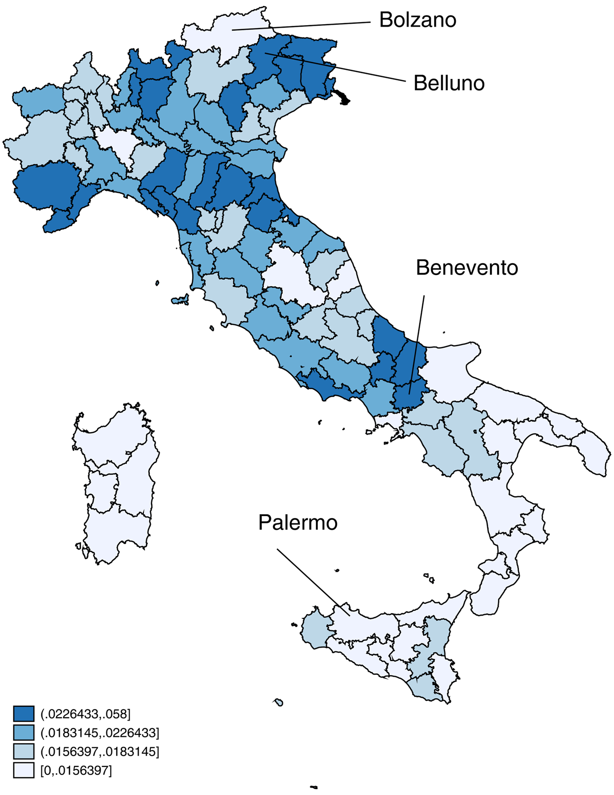
Figure 2. WWII male casualties (soldiers and civilians) as a fraction of resident population in 1936. Note. This figure shows the total wartime male casualties (soldiers and civilians) across Italian provinces as a fraction of the resident population in 1936. Source: ISTAT (1957).
War-related deaths do not follow an obvious geographical pattern, which is most likely the reflection of how drafting was carried out by the Italian Army. According to the 1935 “conscription” (reclutamento) entry of the Treccani Encyclopedia, the drafting was universal and was not based on criteria that may correlate ex-ante with life risk, especially considering that the unfolding of the war events was not predictable at the time of drafting.Footnote 5 One notable exception is between areas that were occupied by the Germans or affected by allied bombing (in Northern and Central Italy) and those areas that were not (all Southern regions excluding Molise and Northern Campania). Our empirical investigation exploits the local variation in the percentage of males who died or were lost during WWII as the driving force of changes in marriage patterns. We also explore heterogeneity in the treatment effect, depending on local conditions.
3. Regression analysis
Our primary units of analysis are marriages. Our primary outcome is a dummy for whether the wife is at least as educated as the husband. We can see from descriptive statistics in Table 1 that, on average, wives are about 1 year less educated than husbands, i.e., finding a wife that is at least as educated favorably compares to the average marriage outcome of husbands. The match behind husband and wife is the result of marriage market bargaining forces, with individuals competing for better partners given the available stock.
Table 1. Descriptive statistics

Note. This table uses data for a sample of individuals married between 1930 and 1955 (1997 ILFI wave). Specifically, we keep parents of ILFI respondents (1,095 marriages) and ILFI respondents (287 marriages) in this time window. Cohorts are indexed to the year of marriage. Before WWII in columns 1 and 2 refers to the sample of marriages between 1930 and 1940. After WWII in columns 3 and 4 refers to the sample of marriages between 1945 and 1955. Panel A reports ILFI demographics. Panel B reports characteristics of the province of marriage in 1931 and 1936, which are obtained from Italian censuses.
We consider the following regression (i is marriage, p is province, t is year of marriage):

where y ipt is the marriage outcome measured by a dummy for whether the wife is at least as educated as the husband, X ipt is a set of controls, i.e., dummies for husband's educational attainment and quadratic polynomials in husband's and wife's age at the time of marriage, μ p is a province effect, γ t is an effect for the year of marriage and, in our richest specification, td r(p) is a linear trend for the region of province p, r(p).Footnote 6
The parameter of interest is φ and measures whether provinces subject to a relatively higher number of wartime casualties experienced a larger improvement of the husband marriage market returns in terms of wife's education, comparing pre- and post-war marriages at the province level. This is identified by including an interaction between the treatment intensity measured by the war-related mortality m p in province p and an indicator for post WWII marriages, POST ipt. Standard errors are clustered at the province level, as this is the level of variation of the mortality variable.
The province-level war shock, m p, is the cumulative number of male deaths during WWII divided by the male resident population in 1936, and it is standardized to have zero mean and unit variance in the sample. We maintain the identifying assumption that assortative matching resulting in a marriage would have changed similarly across provinces from before to after WWII, net of compositional differences in the population at baseline, had all provinces experienced the same war shock (or had WWII not happened). The fact that the shock is as good as randomly assigned across provinces in the same region, as we will discuss below, corroborates the validity of this assumption. We also rely on the assumption that WWII did not affect educational attainment of males and females in a different fashion. This is confirmed by the inspection of the educational patterns' dynamics in Italy around the war years in Figure 3. Any difference in education within couples should then be imputed to changes in matching patterns rather than a direct selective effect of war on husbands' education.

Figure 3. Educational attainment of spouses before and after WWII. Note. This figure shows the educational level (years of schooling) of male and female spouses by year of marriage (from 1930 to 1955). Source: 1997 ILFI data.
4. Data
4.1 The Italian Household Longitudinal Survey
We used data from the Indagine Longitudinale sulle Famiglie Italiane (ILFI; the Italian Household Longitudinal Survey), a longitudinal survey started in 1997 by the University of Trento, the Istituto Trentino di Cultura, and the Italian National Bureau of Statistics (ISTAT).Footnote 7 This survey consists of a sample of 9,770 individuals, in 4,457 households, representative of the national population. We used only the 1997 wave, as this is the closest year to WWII. ILFI is a unique source of data for our research question and has been given scant attention by economists to date. For all interviewees, retrospective information is available about educational choices, employment, family, and residential history over their life. Importantly, information on the socio-economic background of the family of origin is also collected.
Since the first ILFI wave was carried out in 1997, i.e., 52 years after the end of WWII, only few respondents are old enough to have entered the marriage market around WWII. Luckily, we also have retrospective outcomes and demographics for parents of ILFI respondents. However, although information on the socio-economic background and the year of birth of parents is collected, the ILFI questionnaire does not elicit the wedding year of the parents. In what follows, we proxy this variable with the year of birth of the ILFI respondent or that of his/her first-born sibling. The implicit, but reasonable, assumption here is that the time lag between marriage and the birth of the first child was negligible in the years around WWII.
Our working sample consists of two groups of individuals married between 1930 and 1955. Specifically, we keep both parents of ILFI respondents (1,142 marriages) and older ILFI respondents (288 marriages) falling in this window. Cohorts in our analysis are indexed to the year of marriage, which varies in a time interval of plus/minus 12 years from 1943 (the mid-WWII year). This choice leaves us with a sample of 1,430 marriages for which summary statistics are presented in Table 1, separately for the pre- and post-WWII cohorts.
The original ILFI sample aligns well but not perfectly with other surveys collected by the Italian Statistical Office (ISTAT). For example, ILFI manuals show that participants were slightly younger and more educated than the average individual in the national population. In addition, our analysis relies mostly on fathers and mothers of ILFI respondents. Information on the parental generation is self-reported by ILFI respondents, and in principle this may add some additional imbalance. These facts may raise some concerns about the representativeness of our dataset. For example, our data may not be representative of all marriages in the relevant time window, because participation in the ILFI survey is conditional on having children that survived the post-war period.
To shed light on the possible implications of these issues, we compare the age distribution at marriage of parents of ILFI respondents to the age distribution at marriage in official ISTAT Census publications before and after WWII. This comparison can be seen in Appendix Figure A.1. Age distributions for males and females in this figure present some differences, with males being slightly older and females younger in our sample. A possible explanation is that these differences are somewhat the mechanical consequence of the ILFI sampling frame, as discussed above.
Differential mortality in ILFI respondents would likely yield changes in ILFI/ISTAT differences in pre- and post-WWII panels. However, ILFI/ISTAT differences in the age at marriage of the parental generation of ILFI respondents remain the same for ILFI respondents born before and after WWII.Footnote 8 We conclude that, aside from a number of limitations arising from the original sampling frame, we do not find any strong evidence that ILFI respondents were differentially selected depending on their year of birth.
4.2 Census and other administrative data
Survey information from ILFI was combined with data from four different population censuses: 1931, 1936, 1951, and 1961 [see ISTAT (1933), (1937), (1954), (1963)]. The different sources were merged using the province of marriage reported in ILFI. As a result of the loss of the Istrian territories, sanctioned by the Paris Peace Treaty in 1947, we consider 90 administrative provinces that can be matched before and after the war.
Key in our analysis is information on war casualties coming from ISTAT (1957), which contains detailed data at the national and provincial levels on war-related dead (both military and civilian) and missing from June 10th, 1940 to December 31st, 1945. The publication contains time series data at the national level accounting for places of death, causes of death, and other characteristics of the deceased. In addition, province-level statistics are provided by province of birth, province of residence, and province of death (for both soldiers and civilians).
We also analyze the association between the value of dowries and the WWII shock at the regional level using data from ISTAT (1955) on the economic value of dowries for the period 1940–1948 and for all Appellate Court Districts (Distretto di Corte di Appello), which largely coincide with either regional or provincial boundaries.
5. Descriptive and graphical evidence
The marriage market was largely frozen during WWII, especially for younger age groups, as shown in Figure 4. WWII marked a tremendous shock on the lives of young Italians at the time, not only because of the direct involvement in combat of young males but also because of the devastation and suffering that followed on Italian soil. This resulted in dramatic consequences with regard to marriage patterns. At the time males were used to marrying generally later than females, more frequently in their late 20s, compared to females who married more in their early 20s.

Figure 4. Number of marriages over time by age at marriage. Note. This figure shows the time series of the number of marriages (in logs) by age at marriage, for men (left-had side panel) and women (right-hand side panel), using all cohorts in the sample. Source: Italian censuses for 1936, 1951, and 1961.
During the war, both males and females chose to postpone their marriage choices to better times, as shown in Figure 5. The reduction in marriages from 1940 to 1945 was in part offset by the increase in post-war years. Indeed, in the years following 1945 both males and females married at older ages if compared to their peers in pre-1945 years. However, the conditions of the marriage market were then changed due to the consequences of the war. The loss of lives, mainly concentrated on young male soldiers and combatants, determined an imbalance in the gender composition of the marriage market's active population. The surviving single males actively searching for a spouse found themselves in a better bargaining position given the relative decrease in the supply of males with respect to females.
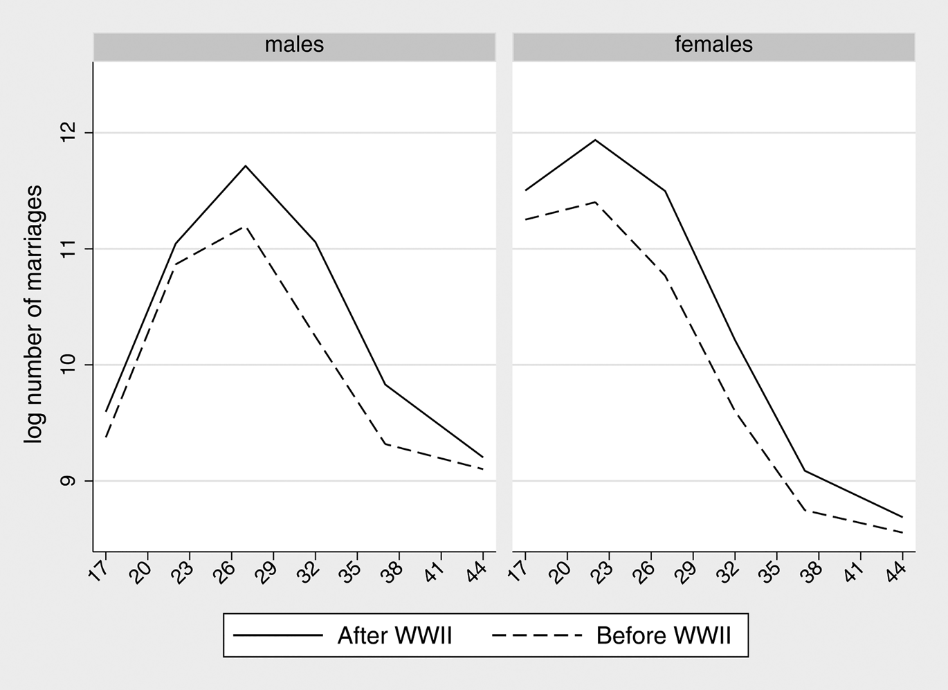
Figure 5. Age at marriage profiles. Note. This figure shows profiles for the number of marriages (in logs) by age at marriage, for men and women. The cohorts used in the empirical analysis are grouped before and after 1945. Source: Italian censuses for 1936, 1951, and 1961.
Figure 6 uses census data to show how the sex ratio changed across Italian provinces between 1936 and 1951. A negative trend emerges, with sizeable variation across provinces. As shown in Figure 2, the incidence of war-related male deaths did not follow a clear geographical pattern, if we exclude the fact that post-Armistice battles on national soil mainly took place in Central and Northern Italy. However, if we consider within regional variation, Figure 2 also shows great variation in the distribution of war casualties. This variation most likely reflects random events such as the composition of army battalions and their world areas of deployment (with Russia and the Balkans being the deadliest) as well as the development of war events across the peninsula and within each region.
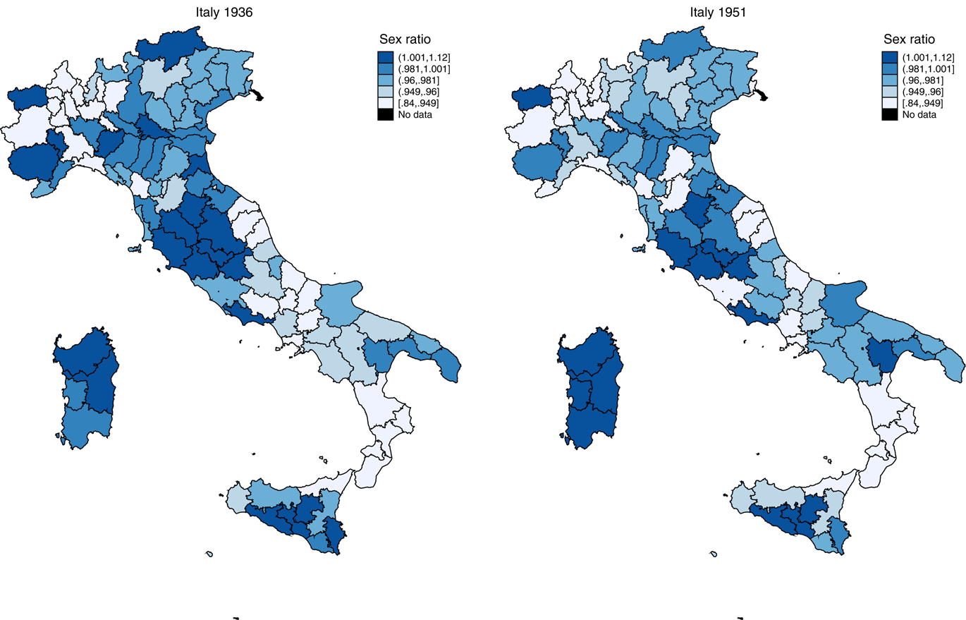
Figure 6. Sex ratio in 1936 and 1951 across Italian provinces. Note. This figure shows the sex ratio (the relative number of men and women) across Italian provinces in 1936 and 1951. Values of sex ratios are grouped using 1936 quintiles, with darker colors representing higher quintiles. Source: Italian Censuses 1936 and 1951.
Similar patterns hold at the municipality level. Figure 7 displays sex ratios for all Italian municipalities (about 7,300, administratively defined as “comune”) from 1936 and 1951 Census data.Footnote 9 Looking at the linear fit in the figure, a general reduction in the sex ratio is evident (the estimated slope being about 0.6). Figure 6 displays changes to sex ratios for the total population. However, these changes may be even larger if we consider only the population actively engaged in the marriage market. Although the dead and missing civilians were mostly concentrated among the very young (under 20) and the mature (above 50), dead and missing soldiers were mainly those between 20 and 30, i.e., those males who may better represent potential candidates for marriage [ISTAT (1957)].

Figure 7. Sex ratio in 1936 and 1951 across Italian towns. Note. This figure shows the sex ratio (the relative number of men and women) across Italian towns (comune) in 1936 and 1951. The linear fit is from a regression of sex ratio in 1951 on sex ratio in 1936. Source: Italian censuses for 1936 and 1951.
A well-known fact about Italy is its regional differences. Maps in Figure 8 provide a visual inspection of pre-war differences across Italian provinces along several dimensions using the 1936 census. Panel A shows that population was concentrated around the largest and most important towns, such as Genova and Milan in the Northwest, Venice and Trieste in the North-East, and Florence, Rome, and Naples in the Center-South. Vast areas characterized by very low density extend over the mostly Alpine region of Trentino-Alto Adige, in Eastern Piemonte, Southern Tuscany, Umbria, Northern Puglia, Basilicata, and Sardinia.

Figure 8. Pre-war province characteristics. Note. This figure shows population density (panel A), the share of employment in agriculture (panel B), the share of illiterate men (panel C) and women (panel D) and mean altitude (panel E) across Italian provinces. Source: Italian census for 1936 (panels A, B, and E); Italian census 1931 (panels C and D).
Variability in population density should not be confounded with a simple industrial vs. agricultural classification of provinces. Panel B of Figure 8 displays the employment share in agriculture that, despite being correlated with low levels of urbanization, presents some interesting variation. The largest employment shares in agriculture were mostly concentrated along the Apennines, with clusters scattered along all latitudes and in the Northern regions, especially Piemonte, Emilia Romagna, Veneto, Trentino, and Friuli.
The most important social divide between Northern and Southern regions in the early 1930s was illiteracy. Panels C and D of Figure 8 shows the illiteracy rate for men and women in 1931, picturing a vastly illiterate South compared to a much more literate North. The difference is huge and striking in some Southern provinces the illiteracy rate could reach almost 60% for women and 50% for men. In the North, provincial illiteracy rates could be as low as 2% for both genders.
To capture a key aspect of Italy's diverse geography that may influence marriage market efficiency, panel E of Figure 8 displays average provincial altitude. Arguably, in more mountainous areas, interaction across villages and towns is less pronounced than in the plains where transport is easier all year round.
Provincial characteristics do not predict the change in sex ratios from before to after WWII, as shown in Table 2. Column 1 here reports results from a regression of the ratio between the sex ratios in 1951 and 1936, computed by province, on region dummies (to capture differential severity of the war across different broad areas of Italy) and province-level variables capturing the degree of development measured before WWII. More precisely, these variables consist of population density in 1936, employment shares in agriculture and industry in 1936, illiteracy rate in 1931, and province altitude, latitude, and longitude. There are regional patterns in the changes in sex ratios, as can be seen from the p-value of the joint significance of the coefficients on region dummies. This finding reflects the fact that the war was overall more severe in the North and Center of the country, as we saw in Figure 2. However, provincial characteristics are not significant in the regression conditional on region-fixed effects. In column 2, we use the male casualty rate as an outcome and ask the same question: can we predict variation in war casualties across provinces within regions by provincial characteristics? The answer is again negative: provincial characteristics do not predict war casualties. We take this as evidence supporting our use of the male casualty rate as our war shock variable. In other words, we consider the within-region male casualty rate as an exogenous shock.
Table 2. WWII casualties and pre-war census demographics
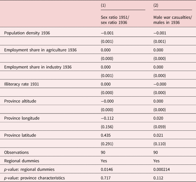
Note. Province-level data are used to run regressions of outcomes on population density in 1936, employment shares in agriculture and industry in 1936, illiteracy rate in 1931, and province altitude, latitude, and longitude. Column 1 shows results when the ratio between the sex ratios in 1951 and 1936 is considered on the left-hand side. Column 2 shows results when the WWII male casualty rate is considered on the left-hand side. All regressions control for a full set of 20 regional dummies, and standard errors in parentheses are robust to heteroskedasticity. ***p < 0.01, **p < 0.05, *p < 0.1.
Finally, our data weigh against any gendered effect of WWII on the educational attainment at marriage. This can be seen from Figure 3, which presents the average education of male and female spouses in the sample by year of marriage (from 1930 to 1955). The educational levels of spouses follow a very similar pattern, with a general positive trend. This evidence supports the idea that WWII had indeed an impact on the sex ratio but not on educational attainment of married males with respect to married females. This in turn suggests that any empirical finding pointing to an effect of the war shock on the difference in educational attainment between husbands and wives should be imputed to the change in the relative bargaining power of males with respect to females, rather than to any direct effect of the shock on educational patterns.
6. Results
6.1 The war shock and marrying up
Table 3 reports our first set of estimates. The first three columns use as outcome the wife's years of education, whereas in the last three columns the outcome is a dummy for whether the wife is at least as educated as the husband. As seen from the descriptive statistics, on average, wives are about 1 year less educated than husbands, therefore finding a wife that is at least as educated favorably compares to the average marriage outcome of husbands.
Table 3. WWII intensity and marriage market
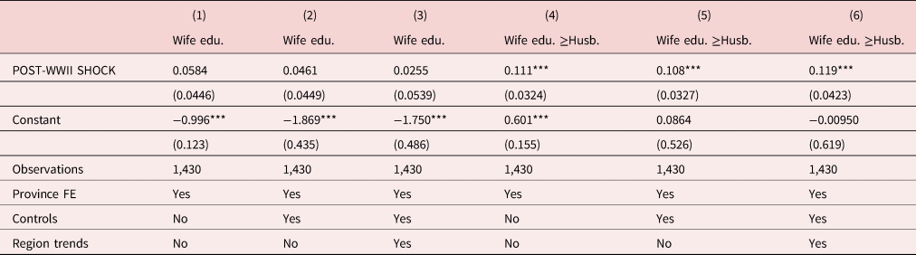
Note. This table shows results from baseline regressions. The outcome is wife's years of education in columns 1–3 and a dummy for whether the wife is at least as educated as the husband in columns 4–6. The variable POST-WWII SHOCK is an interaction between WWII intensity, which is measured by mortality in each province, and post-war dummy POST. The province-level war shock is the cumulative number of male deaths during WWII over male resident population in 1936, and it is standardized to have zero mean and unit variance in the sample. The set of controls at the marriage level include dummies for husband's educational attainment and quadratic polynomials in husband's and wife's age at the time of marriage. In addition, a set of province-fixed effects, marriage dummies and, in our richest specification, regional level linear trends, are included. Robust standard errors, reported in parentheses, are clustered at the province level, as this is the level of variation of the mortality variable. ***p < 0.01, **p < 0.05, *p < 0.1.
Our baseline specification, in columns 1 and 4 of Table 3, includes on the right-hand side of equations a full set of province-fixed effects, a full set of indicators for educational attainment of the husband, and a dummy for observations referring to ILFI respondents as opposed to parents of ILFI respondents, as we explained in Section 4.1. Columns 2 and 5 of the table add quadratic polynomials in husband's and wife's age. Our preferred specifications are the ones in columns 3 and 6, where in addition to the variables above we include region-specific linear trends for the twenty administrative regions of the country. As the WWII shock variable in the regressions is standardized to have mean zero and unit variance, all coefficients in Table 3 should be interpreted as the causal effect of a one standard deviation (σ for short) increase in the province-level mortality rate on the outcome of interest, which we standardize as well.
After WWII, in provinces with more male war casualties, husbands were more likely to marry more educated women. For example, a one σ increase in the WWII shock in column 1 increased by about 6% σ women's education at the time of their wedding. In column 4, the effect on the probability of wives being at least as educated as their husband is about 11% σ. The WWII shock intensity pushed both our outcomes up, although the effect was statistically significant only for the latter “marrying up” outcome, as is evident from the last three columns of Table 3. These are our preferred columns in the table because they directly relate a wife's and husband's education. The general conclusion remains valid across specifications, although differences in effect size across outcomes become slightly stronger when regional trends are controlled for in the analysis.
6.2 Heterogeneous effects across provinces
Results in Table 3 assume that a WWII shock of similar size affected all provinces in a similar fashion, i.e., that irrespective of the structural and institutional characteristics of each province and its local marriage market, an increase in the bargaining power of males accounted for identical gains in terms of the resulting matches.
We investigate the possible heterogeneity arising from market density and other factors along the urban/rural dimension. A number of mechanisms may be at play here. A first source of heterogeneity may stem from the fact that while in rural areas individuals were constrained to meet fewer potential marriage partners, urban areas were characterized by more dynamic inter-personal relationships and may in principle offer more scope to take advantage of fewer males on the marriage market. In this case, the increased bargaining power of single males may have yielded greater gains in more flexible markets, those where demand and supply met more efficiently because of more potential partners. In addition, in urban areas there should be more room to increase the educational content of the match. For example, a single male may have found it harder to use his increased bargaining power in rural areas, where fewer females were available and average educational attainment was more compressed. In principle this should result in a higher probability of marrying up.
The argument may be reversed. Despite being less efficient than urban markets, since males could meet fewer potential partners, more segmented rural markets were also characterized by lower information asymmetry about potential matches. Yet, the degree of competition in denser urban markets may have been too fierce to exploit the advantage. It may therefore be the case that the males' bargaining power advantage induced by WWII casualties was larger in less urbanized markets as a result.
A further potential source of heterogeneity comes from cultural factors. In more traditional areas there may be no scope for marrying up because of cultural resistance. In these areas, education may have not been such a desirable feature for a woman: husbands may prefer not to marry a more educated wife because of local cultural and social norms that would view that not as an achievement but rather as an inconvenience. For example, this may be particularly relevant in provinces characterized by a strong male chauvinistic sentiment, where the ideal wife would be rather submissive to her husband. In this respect, more education may get in the way of submission. An increased bargaining power for males should then translate in different match features and we might not observe an increase in relative education of wives with respect to husbands.
However, more backward areas may also be characterized by a stronger desire to escape socio-economic disadvantage and increasing the average educational attainment in the family may be one way of improving its economic prospects. This desire may dominate any cultural motive to perpetuate traditional subjugation of females and a more educated wife may be welcomed in rural contexts.
We investigate whether the effect of the war shock was heterogeneous across provinces according to measures of population (and hence marriage market) density or, alternatively, to some cultural and socio-economic factors by areas. Specifically, panels in Table 4 investigate the heterogeneity of WWII effects using four province-level variables measured from the 1936 census: the employment share in agriculture (panel A); the share of residents in the province living in municipalities with more than 10,000 inhabitants (panel B); population density (panel C); average altitude of municipalities in the province (panel D). Table 4 presents results from the same regression specifications considered in Table 3, estimated from mutually exclusive samples defined from the 1936 census variables. The first three columns of each panel show results using provinces with values of the census variable below the sample median; the three remaining columns are for provinces above the sample median. For example, the first three columns of Table 4 consider provinces which in 1936 were relatively less agricultural (panel A), with a lower population share in large urban centers—above 10,000 inhabitants (panel B); less densely populated (panel C), less mountainous (panel D).
Table 4. Heterogeneous effects of WWII intensity across provinces

Note. This table presents regressions for heterogeneous effects along the following provincial characteristics: employment share in the traditional agricultural sector (panel A), population share in province living in towns with over 10,000 inhabitants (panel B), population density (panel C), and altitude (panel D). Results in columns 1–3 are from regressions for observations with provincial characteristics below the sample median. Columns 4–6 are for values of the provincial variable above the sample median. The outcome is a dummy for whether the wife is at least as educated as the husband. See Table 3 footnote for a definition of the remaining variables. Robust standard errors, reported in parentheses, are clustered at the province level, as this is the level of variation of the mortality variable. ***p < 0.01, **p < 0.05, *p < 0.1.
What is the reason for studying WWII heterogeneity along these dimensions? Population density is a possible proxy for market density. Denser areas are characterized by more intense exchanges between supply and demand on the marriage market, and therefore outcomes may more easily reflect the bargaining power structure of each player due to this agglomeration effect [Glaeser (Reference Glaeser2011)]. Such a simple density measure may however hide the specific characteristics of demographic distribution across the province, for example due to the fact that areas outside large towns may be characterized by low population densities, despite being part of a province where the overall population density is high. As our main measure of urban–rural divide, we therefore use the proportion of the population in the province living in towns of more than 10,000 inhabitants, which corresponds to ISTAT's definition of large municipalities.
One relevant dimension that reflects possible cultural and socio-economic factors affecting marriages is the extent of substitution of the traditional agricultural economy with more modern industrial or tertiary activities. Traditionally, the Italian rural society was characterized by a rigid patriarchal structure, with few exceptions [Corti (Reference Corti1992)]. The secular structural transformation of the Italian economy embodies fundamental changes in the way social and interpersonal relationships are conceived, with likely consequences on the relation between male and females, and more generally on the role of women in society. The population living in urban centers was also typically richer and more educated than the one living in rural and more mountainous areas, and therefore a marginal increase in education in the family may have a different impact in those contexts [Felice and Vasta (Reference Felice and Vasta2015), Vecchi (Reference Vecchi2017)]. Figure 8 shows that population density and the employment share in the traditional agricultural sector, despite being correlated, do not coincide.
The share of men marrying up because of WWII was higher in provinces with an above-median employment share in agriculture. This can be seen from Table 4, where the effects in columns 4–6 of panel A are between 15% σ and 16% σ and twice as large as the effects in columns 1–3 (effects in these columns are also not statistically different from zero). Consistent with this finding, the effects in columns 1–3 for panel B are generally much larger for provinces with below-median population share in towns over 10,000 inhabitants (the large coefficient in column 6 of panel B is the only exception to this pattern). The effects by population density in the province overall (i.e., averaging across urban and rural areas), in panel C, are—not surprisingly—less clear-cut. Ignoring statistical significance, point estimates in columns 1–3 of this panel are very similar to estimates in columns 4–6. We show these results for transparency, but we consider the measure in panel B to be the one better capturing the urban–rural divide. Finally, in provinces with above-median altitude, effects are between 14% σ and 17% σ—see panel D—and almost three times as large as in the remaining provinces.
Taking stock of our analysis on effect heterogeneity, we conclude that WWII affected marriage patterns more strongly in more agriculturally dominated provinces, in provinces with a larger share of population living outside large towns, and in more mountainous provinces. In these areas, males were better able to exploit their increased bargaining power than in urbanized and more developed areas. A possible caveat here is that we are underpowered for assessing statistical differences between the first block (1–3) and the second block (4–6) of columns of each panel in Table 4. Formal tests for differences between blocks of each panel—not presented here for brevity—fail to reject the null hypothesis in almost all cases, suggesting that our limited sample is not suited to reach a definite conclusion on effect heterogeneity.
6.3 Dowry patterns across regions
We further investigate the consequences of the WWII shock-induced reduction in the relative supply of males by looking at the regional patterns in post-war dowries. Abolished only in 1975, the institution of dowry was common in Italy around the time of WWII, as it is typical of a patrilineal culture. Dowries consisted of money, properties or other economic valuables that the bride's family used to bring to the groom as a contribution to the economic burden of starting a new family [Fazio (Reference Fazio, De Giorgio and Klapisch-Zuber1996)].Footnote 10 As a result of this custom, the attractiveness of a bride used to be influenced by the economic value of her dowry.
In the context of an increase in the relative scarcity of males generated by the WWII shock, a more valuable dowry would increase a bride's bargaining power in a tight marriage market where potential spouses are scarcer, especially in areas characterized by a more intense shock. This hypothesis can be investigated by looking at the empirical association between the average dowry value and the intensity of the WWII shock, at the regional level.
The data on dowries are provided by ISTAT (1955) for the years 1940–1948 at the Appellate Court District (Distretto di Corte di Appello) level, which is a geographic definition that roughly corresponds to either regional or provincial areas. The data report the occurrence of dowries in each area across four classes of value corresponding to less than 50,000 Liras, between 50,000 and 100,000 Liras, between 100,000 and 500,000 Liras, and above 500,000 Liras. The huge inflation rate that characterized the Italian economy during and after WWII (the consumption price index in 1948 was around 40 times the one in 1940) makes it impossible to compare the frequency of dowries within the same nominal value bracket before and after the war. We therefore present some simple evidence on the cross-sectional association between the WWII shock and the proportion of dowries above 50,000 Liras in 1947 (the year following the 1946 proclamation of the Italian Republic) for 16 regions for which a match between Appellate Court District dowry data and WWII shock data was possible.
Selected descriptive statistics are presented in Table 5, where we see that the number of dowries per 10,000 inhabitants in 1940 and 1947 is typically larger in Southern regions (at the bottom of the table), suggesting that the institution of the dowry used to have a strong cultural connotation. Figure 9 displays a clear positive association between the WWII shock and the proportion of dowries above 50,000 Liras, as one would expect if the brides' families would react to a stronger war shock by increasing the value of dowries in order to boost their daughters' probability to get married when males become scarcer. The evidence is consistent with our findings on marriages, i.e., with males appropriating an economic advantage as a result of their increased bargaining power.
Table 5. Occurrence and economic value of dowries across Italian regions

Note. In columns 1 and 2, the number of dowries is normalized using regional population in 1936.

Figure 9. Average dowry value across regions in 1947 and WWII shock. Note. The data on the proportion of dowries above 50,000 Liras are calculated using 1947 data from ISTAT Statistiche Notarili.
The figure is based on a nominal monetary threshold of 50,000 Liras that is common to all regions despite the presence of different price levels across regions. However, as documented by Amendola et al. (Reference Amendola, Vecchi and Al Kiswani2009), in post-war Italy prices were typically lower in Southern Italy than those in the rest of the country. Nevertheless, the positive association is robust to the exclusion of Southern Italian regions, highlighted in red in the figure. A positive and statistically significant association is also displayed in Table 6, where the proportion of dowries above 50,000 Liras is regressed on the WWII shock, the share of population employed in agriculture and the number of dowries per 10,000 inhabitants which is much higher in the South than the rest of the country.
Table 6. Economic value of dowries and WWII shock

Note. Dep. Var: share of dowries above 50k Liras. Standard errors in parentheses. ***p < 0.01, **p < 0.05, *p < 0.1.
7. Conclusions
We have investigated how the exogenous shock induced by WWII on the sex ratio, i.e., the ratio of males to females, affected marriage patterns across Italian provinces. The number of marriages decreased during the war years, since most marriages were postponed to the post-war years. However, as a result of the war losses sex ratios generally decreased in most provinces. The deaths of young males affected the pre-war equilibrium in the marriage market by reducing the number of available males with respect to females, thereby increasing the bargaining power of surviving single males on the market because fewer males were available as potential partners with respect to females. Within this framework, an increase in the relative scarcity of males, induced by the war shock, should have increased a male's ability to marry a more desirable partner in post-war years.
We have found that after WWII, surviving males in provinces with more male war casualties married relatively more educated women. We have considered potential sources of regional heterogeneity in the way the shock to the marriage market affected marriage patterns. We tested whether the increased bargaining power of single males may allow greater gains in urban markets where, being easier to meet more potential marriage partners, demand and supply meet more efficiently, or in sparser rural markets, where the returns to the shock may be larger due to less information asymmetries, competition, and saturation. In addition, in urban areas there should be more room to increase the educational content of the match, whereas in more traditional areas there may be no scope for marrying up because of cultural resistance. On the contrary, a more educated wife may be welcomed in rural areas, typically characterized by a stronger desire to escape socio-economic disadvantage. We have found that the effect of the WWII shock was more pronounced in sparsely populated, agricultural, and mountainous areas where a larger reduction in the relative supply of males induced by the war imply higher gains for the surviving males with respect to more industrial and urban areas in the plains. We also report a positive association between the WWII shock and the post-war value of dowries across regions, which is consistent with brides' families strategically adjusting the economic attractiveness of their daughters' marriage in order to respond to an increase in the relative scarcity of potential male partners.
These findings contribute to our understanding of marriage patterns and how those are influenced both by the supply of men and women, as well as by marriage market efficiency and cultural factors.
Acknowledgments
We thank the editor and two anonymous referees for constructive suggestions. Our thanks to seminar participants at the University of Padua and FBK-IRVAPP for helpful comments, and to Giovanni Vecchi and Stefano Chianese for helping us locate data on dowries. Andreas Weber, Marco Bertoni, Costanza Bruno, Stefano Fiorin, Martina Miotto, and Veronica Toffolutti provided invaluable research assistance to access World War II and census data from the Italian National Bureau of Statistics (ISTAT). This research was supported by the University of Padua “Progetti di Ateneo.”
Appendix
See Figure A.1.

Figure A.1. Age distribution at marriage in ILFI sample versus census data.
Note: This figure compares the age distribution at marriage of males and females before and after WWII, in our ILFI estimation sample, and in census data collected by ISTAT.


 Open access