The return to risky corporate debt plays an important role in many controversies about the macroeconomic history of the war and interwar years. It is discussed, to list some prominent examples, by Milton Friedman and Anna Schwartz (Reference Friedman and Schwartz1963, pp. 245–48, 312), Peter Temin (Reference Temin1976, pp. 96–103, Reference Basile1989, p. 54), Ben Bernanke (Reference Bernanke1983), Frederic Mishkin (Reference Mishkin and Glenn Hubbard1991), Charles Calomiris (Reference Calomiris1993), Peter Ferderer and David Zalewski (Reference Ferderer and Zalewski1994), Elmus Wicker (Reference Wicker1996, p. 40), and Allan Meltzer (Reference Meltzer2003, pp. 519–20). The issues discussed range from a possible decline in lending standards in the 1920s, to the effects of monetary policy in the 1930s, and to the effects of the world wars on the civilian economy. Students of this period, however, have been forced to rely on an index of the yields of Baa corporate bonds to measure risk because this is the lowest quality bond for which an index has been constructed that covers most of the twentieth century.Footnote 1 As shown in Table 1, however, Baa bonds were relatively high on Moody's scale: during the interwar years Moody's described Baa bonds as “good quality.” Conceivably, the Baa yield is sufficient to tell us all we need to know: The yields on higher risk securities could be simple multiples of the Baa yield. But to be certain that we have a full picture of the risk structure of the bond market we need information on lower rated bonds.Footnote 2
Table 1 BOND RATINGS
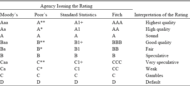
Notes: Junk bonds are often defined as those rated Ba or below. Our index is confined to bonds rated B or below. Defaulted bonds are excluded. The verbal descriptions are those used by Moody's during the period 1910–1955.
Source: Hickman (Reference Hickman1958, p. 142).
Here we present a new monthly index of junk bond (high risk) yields for the period 1910–1955 and describe how it was constructed.Footnote 3 We then show that there is important information in the junk bond index which is not present in the Baa index and argue that re-examining the received macroeconomic wisdom in the light of this index is likely to pay dividends.
CONSTRUCTION OF THE JUNK BOND INDEX
Junk bonds (or high yield bonds to use a term more likely to encourage someone to buy one!) are corporate bonds that have high yields to maturity because of high risks of delayed or reduced payments, or outright defaults. An operational definition makes use of the ratings assigned by one of the rating agencies. Today, typically, junk bonds are defined as those that are rated Ba or below by Moody's and Bb or below by Standard & Poor's. Here, however, we restrict ourselves to bonds that were rated B or lower by Moody's in order to focus on bonds that were clearly risky investments.
Richard Sylla (Reference Sylla, Levich, Majnoni and Reinhart2002) has described the history of the rating agencies. The U.S. bond market was around 100 years old when John Moody published the first ratings (essentially letter grades for bonds) in 1909, a date that determines the beginning of our series. Investors, of course, had access to information before formal ratings were issued. Credit reporting agencies (that published information about the credit worthiness of businesses), the financial press, and investment bankers who provided implicit guarantees as they distributed securities, all supplied valuable information to potential investors. But at the turn of the century the widening market for securities, and perhaps growing skepticism about the advice provided by investment bankers in the wake of the Panic of 1907, expanded the market for the easy-to-use and apparently arms-length ratings that Moody provided. Poor's Publishing Company, a publisher of information about railroad bonds, began issuing ratings of railroad bonds in 1916. Standard Statistics began issuing ratings of non-railroad bonds in 1922. The two merged in 1941 to form Standard & Poor's. Fitch Publishing Company, the smallest of the rating agencies, began issuing ratings in 1924. Fitch rated a smaller number of bonds than the other firms. For consistency, and to start at the earliest possible date, we have used Moody's ratings.
In constructing the index, we have followed the methodology developed by Frederick Macaulay (Reference Macaulay1938) in his classic study of interest rates in the nineteenth and early twentieth centuries. Although Macaulay's methods were developed long ago, there are several advantages in using his work as a model. Many of the problems that Macaulay faced as he pushed his index back into the nineteenth century—a limited number of securities, missing prices, thin markets, and so on—are similar to the problems one encounters in computing an index of junk bond yields. Macaulay used his methodology to compute rates of return on railroad bonds, the most important security in U.S. bond markets, from 1857 to 1936.
Macaulay's series are still used by economic historians, especially when exploring rates in the second half of the nineteenth century through WWI: for example, Friedman and Schwartz (Reference Friedman and Schwartz1982, p. 110), Maurice Obstfeld and Alan M. Taylor (Reference Obstfeld and Taylor2003), and Scott Mixon (Reference Mixon2008). However, all of the bonds that Macaulay used were relatively high quality. To examine the effects of quality on his yields Macaulay (Reference Macaulay1938, pp. A110–12) computed three indexes of the yields of the five highest quality (lowest yielding) bonds and three indexes of the five lowest quality (highest yielding) bonds in his sample. It might be possible, therefore, to use Macaulay's indexes of low quality railroad bonds as a proxy for junk bonds. Unfortunately, however, this does not work. All three indexes of Macaulay's lowest quality bonds were lower (indicating higher quality) than Moody's Baa index in every year from 1919 to1936 when all are available. On average over 1919–1936 Aaa bonds yielded 4.80 percent and Baa bonds yielded 6.77 percent, while the average of Macaulay's indexes of his lowest quality bonds were 5.61, 4.28, and 4.79 percent, respectively. Evidently, despite Macaulay's path breaking work, we still need an index of risky bond yields.
In general, we chose bonds with characteristics that were similar to those in the workhorse Aaa and Baa indexes except for rating. The goal was to be able to interpret differences in yields between junk bonds and higher rated bonds as differences in the market's evaluation of risk. More specifically we chose bonds with the following characteristics.
First, the bonds were rated B or lower by Moody's. As noted, this assures us that all the bonds in our index were regarded as risky, speculative investments. Second, they had maintained their rating for three or more years. By using this criterion we avoid volatility being imparted by bonds that were moving rapidly up or down the rating scale. A similar criterion was used in choosing bonds for the workhorse Baa indexes. The term for these bonds was “seasoned.” Third, they were ten or more years from maturity. When the term to maturity fell to less than ten years, they were replaced by bonds with longer maturities. This ensures that the duration of the bonds in the junk bond index was as similar as possible to the bonds in the Baa indexes and, therefore, that changes in the shape of the yield curve would not influence the gap between junk and Baa bonds. Fourth, the bonds we used had call, convertible, or sinking fund provisions. This was typical of most junk bonds and many higher rated bonds at the time. When rates declined in the 1930s many corporations took advantage of the call provisions and refinanced. W. Braddock Hickman (Reference Hickman1958, p. 7) found that 37 percent of his sample of corporate bonds issued between 1900 and 1943 had been called. The presence of these provisions were known to buyers and reflected in the prices they paid for the bonds. A corporation's decision to exercise a call provision was a risk for the buyer of a bond that was similar to the risk of default: when the bond was called, the bondholder would be paid the face value of the bond, but would have to reinvest, most likely at a lower rate. In principle, one could estimate the effects of these provisions and isolate the default risk, but we have not tried to do so, and no estimates of this sort are available for the higher rated bonds for comparative purposes. Fifth, to maintain comparability with the workhorse Aaa and Baa yields, we chose bonds from the same sectors of the economy. This meant using railroad bonds for the period 1910–1918, and railroad, industrial, and public utility bonds in the following years.
Prior to 1928 the price of a bond was the asking price from the General Quotation section of the Commercial and Financial Chronicle (Chronicle). From 1928 on, actual sales prices from the Chronicle were used because they had become available. The Chronicle (for example, 5 January 1929, vol. 128, p. 44) claimed that its tables were “all compiled from actual sales.” And there are many blanks in the tables suggesting that when the Chronicle did not have a sale it did not report a price. But to be on the safe side we excluded bonds that had more than two consecutive quarterly price quotations that were the same. These repetitions might have reflected the actual transaction history, but repetition also might have reflected an attempt to guess at a price when transaction information was incomplete, or possibly that a simple recording error had been made.
We used Macaulay's system for chaining yields when it was necessary to change securities because (1) the term to maturity grew too short, (2) the bond went into default, (3) price quotations were not available, or (4) one of the other criteria could not be met. New bonds were added in January, and the average yield for each subsequent observation during the year was multiplied by the ratio of the average yield on the old sample of bonds in January to the yield on the new sample in January.
In the period 1910–1920 the number of bonds that fulfilled all of the criteria and were included in the index varied between 6 and 13, averaging 9. In 1921–1930 the number varied between 5 and 13, averaging 8; in 1931–1940 the number varied between 9 and 24, averaging 14; and in 1941–1955 the number varied between 14 and 31, averaging 20. The number of bonds used in each month is reported in the Online Appendix.
Perhaps the most important concern for someone using the index is whether the sample of junk bonds had to be changed so frequently because of defaults that the resulting index is qualitatively different from the Aaa and Baa indexes. The indexes of the yields of safer assets also change as securities are added or removed, but it could be that the substitutions were more frequent and more disruptive for the junk bond index. Defaults on junk bonds, however, were surprisingly rare during the period covered by our index. This was one of Hickman's (1958) basic findings. It is interesting to note, by the way, that Michael Milken, the “Junk Bond King,” relied on Hickman's finding to make his case for investing in junk bonds. Nevertheless, we addressed this concern by computing a simple average of all junk bond yields available each month. The resulting “unchained” series, which is available in an Online Appendix, appears nearly congruent with the chained index when the two are plotted. There are only a few small visible differences at the height of the Great Depression. We also computed an unchained geometric average. The potential benefit of the geometric average is that it is less likely to be distorted by outliers (e.g., bonds on the verge of default) than an arithmetic average. However, the unchained geometric average was also nearly congruent with our chained index. It is also available in the Online Appendix.
Junk bonds represented only a fraction of the total capitalization of the bond market during our period, but it was by no means a trivial fraction. In the years from 1912 to 1944 examined by Hickman (Reference Hickman1958, p. 150), bonds rated Ba or below on average made up about 22.6 percent of the book value of outstanding rated bonds.Footnote 4 The peak was 1940 when bonds rated Ba or below accounted for 41.5 percent of the book value of outstanding rated bonds. Some of the bonds rated Ba or below were “fallen angels,” bonds that had started out as highly rated bonds and been downgraded. But the notion that junk bonds are mostly “fallen angels” is based on the modern junk bond market. In the 1910s and 1920s many bonds were issued with low ratings. Lea V. Carty (Reference Carty2000, p. 73) found that in the 1920s bonds frequently received B ratings when issued, and to judge from Carty's Figure 1, over a thousand were first rated B, “speculative.” The firms that issued junk bonds, moreover, were closer on the risk spectrum to the mass of firms that were too small to issue bonds at all, and that relied on banks or the informal capital market for funds (Wilhelm Reference Wilhelm1945, pp. 222–34). So the information provided by the junk bond index may describe the experience of more firms than just those that were explicitly rated.

Figure 1 BOND YIELDS, MONTHLY, 1910–1955
Our index of junk bond yields, we should add, is not designed to reflect investor experience. It does not tell us, for example, how an investor who bought a particular portfolio would have fared if the investor had held those bonds to maturity. Rather, the index is constructed to measure the cost of capital for risky firms at a point in time. It is most useful for understanding the channels through which economic policies affect investment spending and related variables.
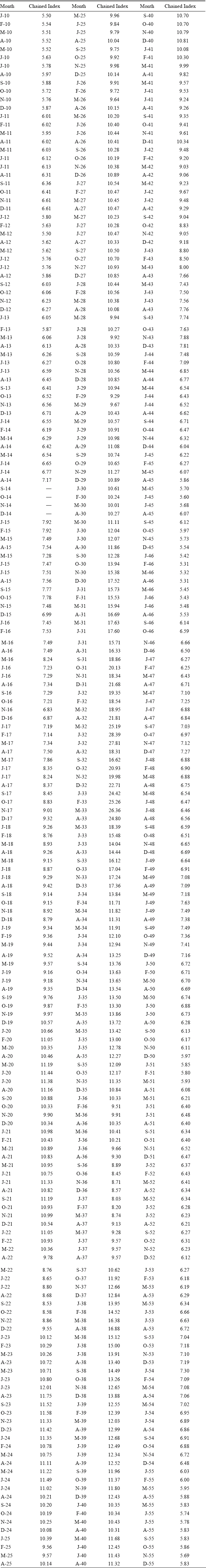
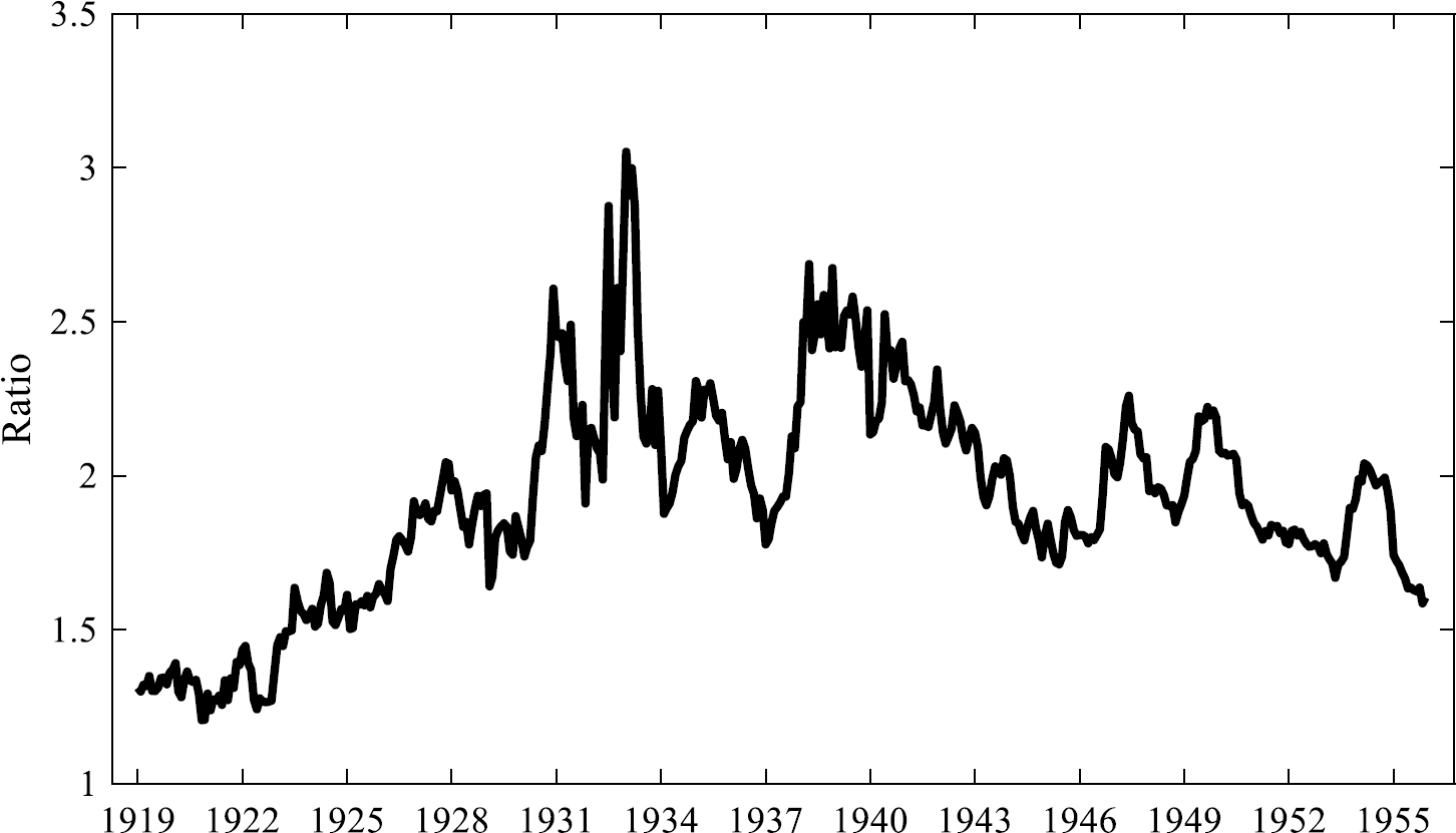
Our index of junk bond yields is plotted in Figure 1, along with the yields of long-term government, Aaa, and Baa bonds.Footnote 5 The underlying index values are reported in Appendix Table 1. Clearly the Baa index contains much of the information in the junk index. However, the junk bond rate is not a mere simulacrum of the Baa rate. Consider the following example. The Baa-Aaa gap peaked during the 1920–1921 contraction at about 351 basis points. This level was not surpassed until April 1931. The Junk Bond-Aaa spread, on the other hand, surpassed its February 1922 peak of 643 basis points a year earlier. Over the period when both Moody's Baa and the Junk indexes are available, January 1919 to December 1955, the correlation between the levels in the two series is 0.79 and the correlation of the month to month percentage changes is 0.64.
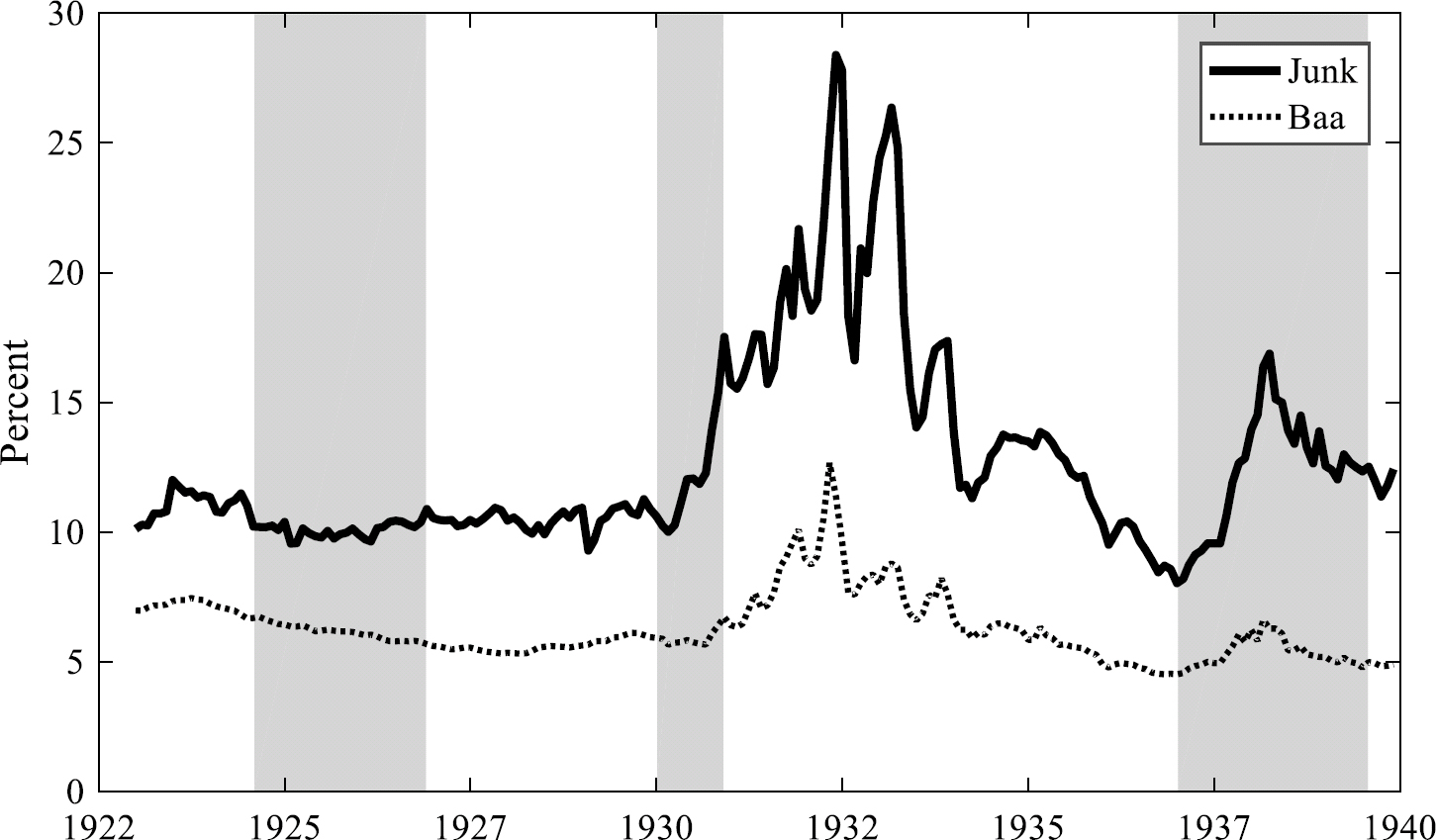
To facilitate a comparison of the Junk and Baa rates we have plotted the ratio of the two in Figure 2. Several segments of the years covered in the figures deserve special attention because they have been explored by economic historians who were forced to rely on the Baa rate, and which therefore might be worth reexamining using our junk bond rate. We cannot, of course, pursue full investigations here, but we can suggest some avenues for future research that we think would be highly productive. Three segments in particular are highlighted in Figure 3, which omits the Aaa and government series and limits the time frame to make it easier to focus on these periods.

The first period of interest is the mid-to-late 1920s when the junk bond rate remained high and stable in contrast to the Baa rate which declined. An exploration of this divergence may throw additional light on the controversy over whether lending standards declined in the late 1920s because the junk bond index provides systematic evidence on how market participants priced risks separately identified by the rating agencies. Geoffrey Moore (Reference Moore1956) surveyed the literature. Friedman and Schwartz (Reference Friedman and Schwartz1963, pp. 245–48) re-examined the issue and suggested that looking at yields by rating may be the best way of addressing the issue. This can be done with our junk bond series.
A second period of special interest is the infamous year 1930. Several economic historians have examined the Baa rate, which began a slow rise in October 1930, to understand the nature of the crisis that was unfolding. Friedman and Schwartz (Reference Friedman and Schwartz1963, p. 312) argued that the increase in Baa rates reflected the effects of the first banking crisis: banks were probably disposing of risky bonds to strengthen their liquidity position. Temin (Reference Temin1976, pp. 103–21), dissatisfied with the Baa index, constructed a biannual index for 1929–1931, and argued on the basis of it that yields began to rise before the banking crisis. Wicker (Reference Wicker1996, p. 40), also examined the Baa rates, and concluded that although there was a small increase in late 1930 the bond market remained “calm and orderly.” As seen in Figure 3 junk bond yields began to rise sharply in April 1930, before Baa yields, suggesting that investors had already become aware that an unusually severe economic contraction was taking hold.

The extraordinary increase in junk bond yields during the period 1931–1933 reinforces what we know: the Great Contraction was uniquely severe. But a third puzzling segment is the recession of 1937–1938 and the months following up to the outbreak of the war in Europe. Considerable interest has attached to this period because of Bernanke's (Reference Bernanke1983) contention that the Depression persisted because the cost of capital for bank borrowers remained high rather than returning to pre-crisis levels. Examination of this thesis, however, has been hampered by the lack of an adequate measure of the cost of capital for smaller firms. Measured bank lending rates do not show much of an effect from the banking crisis (Smiley Reference Smiley1981; Bodenhorn Reference Bodenhorn, Bordo and Sylla1995), perhaps because banks turned sharply away from financing high risk borrowers. And the Baa rate, which rises modestly during the 1937–1938 recession and then quickly subsides to levels similar to those of the late 1920s, also does not show much of a continuing effect from the crisis. But as Bernanke pointed out, it is not convincing as a proxy for the cost of bank credit intermediation because it applies to large companies with relatively high credit ratings. On the other hand, we can see in Figure 3 that our junk bond rate, which as we noted is a better proxy for the cost of credit to smaller firms than the Baa rate, rises sharply during the recession and remains elevated compared with the late-1920s level until the outbreak of WWII, providing additional evidence for Bernanke's argument.Footnote 6
CONCLUSION
Financial historians have long been interested in the returns on risky bonds, but they have hoped that looking at the second rung on the corporate risk ladder, the Baa rate, would provide them with sufficient information. Here we presented a new index of the yields of junk bonds during the tumultuous years from 1910 to 1955. As it turns out, the junk bond yield contains information independent of the information contained in the Baa and higher rated yield series. The junk bond series, we believe, will be useful to economic historians exploring a number of macroeconomic issues in the twentieth century that have been of interest, such as the impact of the world wars and the Korean War on security markets, the evolution of lending standards in the late 1920s, the impact of the onset of the Great Depression on security markets, and the reasons for the persistence of the Depression.
Our examination of the junk bond index has also convinced us that it would be worthwhile extending the index forward and backward in time. By extending it forward we will be able to put the effects of institutional changes—for example, the Milken revolution—into a longer-term perspective. Extending the index backward in time, it must be admitted, will be a somewhat artificial exercise because it will mean extending the index into a period before formal rating systems existed. But we believe that an increased understanding of the price of capital for high-risk enterprises during a period of rapid technological change and economic growth in the nineteenth century would justify the effort.
APPENDIX
Appendix Table 1 JUNK BOND YIELDS, MONTHLY, 1910–1955