


The development of wages has been central to the debate on the impact of economic growth on worker welfare. Much of the discussion has been informed by the surplus-labor and dual-economy models of Lewis (Reference Lewis1954) and Kuznets (Reference Kuznets1955), predicting that unskilled wages remain stagnant or grow at a slower rate than average incomes as surplus labor in rural agriculture holds down incomes of laborers in the expanding urban and industrial sector. Historical evidence also indicates that economic development can lead to a divergence between living standards for the working class and gross domestic product (GDP) per capita (Lindert and Williamson Reference Lindert and Williamson2016; Allen Reference Allen2019). This debate has mostly been informed by the experience of Britain and the United States, making consensus on general conclusions difficult. In this study, we look at Sweden, which is interesting in this context as it has been highlighted as a case where workers benefited from industrialization, but there is a debate on the degree to which this was actually the case.
The study uses a new data set on Swedish construction-worker wages for four groups of workers—helpers, carpenters, masons, and teamsters—during the period of 1831–1900. The data consist of reports on wage rates collected by local fiscal authorities, used by the state to assess the cost of construction projects. The data have a uniquely detailed geographical coverage, including a broad set of places in the countryside as well as a large proportion of towns. The period was a time of significant economic change in Sweden, putting the country on the path to becoming one of the leading industrial economies by WWI. Our new detailed data series allows us to track how the significant shifts in society during the period affected workers’ living standards and to examine several important mechanisms that led to economic change materializing in real wage growth.
We find that real wages were stable prior to the 1850s but grew significantly thereafter. Between 1855 and 1900, real wages for helpers increased by 2 percent per year, outstripping income growth for semiskilled and skilled carpenters and masons, as well as the growth of GDP per capita. Workers, and especially the unskilled, were thus among the primary beneficiaries of Swedish industrialization. To explore whether the Swedish experience was unique, we compare real wages of unskilled workers in Sweden to those of comparable workers in the leading cities of Northern Europe, using the data collected by Allen (Reference Allen2001). We find that by the late nineteenth century, only London had higher unskilled worker wages, with wages in Sweden outperforming those in Amsterdam, Antwerp, and Paris. We then compare levels of real wages to GDP per capita to examine if faster economic growth can explain the Swedish position. We find, to the contrary, that Swedish workers had higher living standards for every level of GDP per capita and that wages in Sweden grew at a much faster rate during the transition to modern economic growth than in the other countries. Even areas with the lowest real wages in Sweden held up well in international comparison.
We find that favorable external factors, such as forces of globalization and mass migration to the United States, combined with well-integrated and flexible labor markets, allowed the working class to reap the benefits of economic growth. This was signified by a lack of surging skill differentials, small urban-rural wage gaps, and a strong convergence of real wages across regions.
In continuing the examination, we organize the paper as follows. The next section discusses previous research into the link between economic growth and inequality. After a brief review of the theories of Lewis and Kuznets, we address the historical experience of Britain and the United States, which has informed much of the debate. This leads to a discussion of studies of inequality, wages, and economic growth, followed by a more detailed look at the Swedish case. In the third section, we present the new database, explain the hedonic wage regression we use to adjust the sample, and describe how we calculate welfare ratios. We proceed using the new database to analyze how economic development affected wages in Sweden. We begin the fourth section by tracking the growth of real wages for the four categories of workers and examine the development of unskilled wages in relation to the evolution of GDP per capita and wages for more skilled groups of workers. We continue by comparing the pattern of real wages for unskilled workers in Sweden to those of the leading cities in Northern Europe. In the fifth section, we look at four possible causes for the robust growth of Swedish wages: the development of nominal wages and prices, the urban-rural wage gap, the convergence of wages across regions, and the effect of overseas migration. We offer conclusions in the final section.
THE LINK BETWEEN ECONOMIC DEVELOPMENT AND INEQUALITY IN THEORY AND HISTORY
Economic Growth and Wage Development
The relationship between growth of GDP per capita and the incomes of the working class has been the theme of several theories in development economics. Two of the most famous are the models developed by Lewis (Reference Lewis1954) and Kuznets (Reference Kuznets1955), who both analyzed the economy in terms of a split between a traditional sector, consisting primarily of rural agriculture, and a modern capitalist sector, dominated by urban manufacturing. In these models, economic development takes off as employment expands and productivity grows in modern industries, while labor shifts away from traditional agriculture. In Lewis’s model, the traditional sector constitutes a source of unlimited supply of unskilled labor, keeping wages down in the modern sector. Inequality increases as capitalists and skilled workers reap the benefits of growing productivity. In Kuznets’s model, traditional sector workers earn a subsistence wage, while incomes for workers in the modern sector grow with increasing productivity. According to Kuznets, inequality is higher in the capitalist sector. Together with growing income differentials between the traditional and modern sectors, the shift of employment toward urban manufacturing leads to rising disparities.
Inspired by the work of Lewis and Kuznets, the impact of growth on wages has been intensely debated in the case of Britain and the United States. In both cases, there is evidence of increasing inequality during the early phases of industrialization. In Britain, the wage share of national income declined after economic growth took off sometime in the middle of the eighteenth century, a phenomenon dubbed by Robert Allen as the “Engels pause” (Allen Reference Allen2009). It was not until at least the 1830s that the working class saw significant improvement in their living standards (Williamson Reference Williamson1985). In the first half of the nineteenth century, the middle class and farmers registered the greatest income gains, while the average real income of workers was stagnant (Allen Reference Allen2019).
The existence of a similar stagnation in wages of common laborers before the Civil War in the United States has been discussed extensively in different attempts to chart the evolution of real wages (Lebergott Reference Lebergott1960; David and Solar 1977). Margo (Reference Margo2000) shows a slower rise than most previous studies, demonstrating that labor wage growth was not as strong as average income growth. Lindert and Williamson (Reference Lindert and Williamson2016) argue that the United States started out with a more egalitarian economy but that inequality grew from the Revolution to the Civil War. Increasing skill premiums and surging urban-rural gaps were major factors.
More generally, the literature on human height as a measurement of living standards has also stressed the importance of going beyond GDP per capita. The early literature on the subject saw human stature as a complement for periods where no estimates of GDP per capita were available, but data showed that height would sometimes fall even in times of rapid economic growth. It was revealed that inequality was an important factor, as height was more strongly associated with wages than with GDP per capita (Baten Reference Baten2000).
In this paper, we use the case of Sweden during its early economic development to illustrate the importance of distinguishing between wages and GDP per capita when comparing prosperity across place and time. We are well positioned to do so, since our data set allows us to look at several different dimensions of the distribution of the benefits from economic growth. Swedish economic history also provides a useful example of significant structural and social change over the course of its early economic development.
The Swedish Economy in the Nineteenth Century
In the nineteenth century, Sweden experienced a classic takeoff in economic growth that resulted in a shift from agriculture to manufacturing and services. An agrarian revolution, which led to radical changes in the social structure in the countryside, predated the process. The number of people without ownership of land—and, as a consequence, the share of people who were dependent on wage work for their upkeep—grew (Myrdal and Morell Reference Myrdal and Morell2011).
From the 1860s, economic growth took off in a major way, originating in raw-material processing activities such as sawmills and ironmaking. Once this transformation began, change was rapid and economic growth soon shifted to higher value-added activities such as metal manufacturing and pulp and paper production. The change away from the primary sector was rapid: Between 1860 and 1900, agriculture as a share of employment dropped from 70 to 50 percent (Lobell, Schön, and Krantz Reference Lobell, Schön and Krantz2008). Early industrialization had a distinctly rural character, but toward the later part of the century, rural to urban migration grew and urbanization increased as economic development became increasingly oriented toward cities (Nilsson Reference Nilsson1989; Lundh Reference Lundh2006; Eriksson Reference Eriksson2015).
The literature on Swedish wages and inequality has been quite narrow in emphasis, focusing mostly on the period from the economic takeoff in the 1860s. Williamson (Reference Williamson1997) found that wage growth outpaced average income growth in Sweden over the 1870–1913 period. He attributes this to open economy forces, where migration to the New World and capital import served to push up unskilled wages. Using differentials in average incomes across sectors, Söderberg (Reference Söderberg, Brenner, Kaelble and Thomas1991), on the other hand, identified a tendency toward increased inequality over the same period. Lundh and Prado (Reference Lundh and Prado2015) used the difference between wages of unskilled engineering workers and agricultural laborers to proxy the urban-rural gap and found a small increase in the period before WW1. Enflo, Henning, and Schön (Reference Enflo, Henning and Schön2014) and Collin (Reference Collin2016) both show that regional inequalities declined in the late nineteenth century, while they were increasing in other countries where comparable information is available (see Figure 3 in Enflo and Rosés Reference Enflo and Rosés2015). The same is true for interindustry differentials for male workers in manufacturing, as presented by Prado (Reference Prado, Edvinsson, Jacobson and Waldenström2010).
The current historiography has focused on the period when Swedish economic growth took off. However, if we are interested in the relationship between economic transformation and wage growth, it is crucial to include the preceding period. Research on the origins of industrialization in Sweden has long stressed the importance of structural change and the fortunes of different social strata in the period prior to industrialization (Fridholm, Magnusson, and Isacson Reference Fridholm, Magnusson and Isacson1976; Schön Reference Schön1979; Sandberg Reference Sandberg1979). For example, Schön (Reference Schön1979) shows how the changing consumption patterns of textiles between the 1820s and the 1850s indicate growing incomes for the poorer segments of the population. Similarly, Gadd (Reference Gadd2000) argues that Sweden had broken away from the Malthusian trap by 1800 and that the growth in the share of landless workers reflected improved possibilities to earn sufficient income without access to land. Sandberg and Steckel (Reference Sandberg and Steckel1997), in turn, highlight how health improved in the decades prior to industrialization, something that is reflected in the height of male conscripts, which rose continuously over the nineteenth century (Öberg Reference Öberg2014). Important institutional changes also took place around the same time, including universal and mandatory schooling, gradual liberalization of labor laws, and increased investment in infrastructure (Lundh Reference Lundh2010; Oredsson Reference Oredsson1969; Sandberg Reference Sandberg1979). The question remains as to what implication this had for wages.
In what follows, we present new, detailed data series on construction workers’ wages in Sweden to examine the living standards of the Swedish working class in a comparative perspective over a longer period of time and how it relates to the economic transformation that took place over the same period.
NEW SOURCE FOR CONSTRUCTION WORKERS’ WAGES, 1831–1900
We present a new database on wages for different kinds of construction workers, which we use to calculate welfare ratios.Footnote 1 The data and approach have several advantages compared to earlier research on Swedish wages for this period.
First, the wages are more consistent and provide more information than earlier data that cover the entire period. The wage series from Jörberg (Reference Jörberg1972), which is the standard reference for the pre-1870 period, has wages only for unskilled farmhands, while our data have information for different levels of skill. Furthermore, our wage data set includes cities, allowing us to calculate urban-rural wage gaps. Earlier research either does not include wages for cities (Jörberg Reference Jörberg1972) or does not have wages for similar types of workers but, rather, compares farm workers with workers from other sectors (Lundh and Prado Reference Lundh and Prado2015), whereas we can compare workers of different skill levels in the countryside with their counterparts in the cities. Our data set also has better geographical coverage than earlier wage series, with wages reported from between 53 and 168 different administrative units around the country, compared to a maximum of 32 for Jörberg.Footnote 2
Some earlier studies have compared Swedish wage levels to those of other countries. Söderberg (Reference Söderberg1987) compares Stockholm to a number of European cities, but stops in 1850; Gary (Reference Gary2018) extends Reference SöderbergSöderberg’s comparison to include the Swedish cities of Malmö and Kalmar. Williamson (Reference Williamson1995) presents wages starting in 1830, but without using them to examine the Swedish case. The analysis of Sweden in O’Rourke and Williamson (Reference O’Rourke and Williamson1995) focuses only on the second half of the century. Furthermore, Reference SöderbergSöderberg uses rye prices to calculate real wages, whereas O’Rourke and Williamson use different baskets for different countries. We are the first to use welfare ratios in the vein of Allen (Reference Allen2001) to compare Swedish wages to other countries during the nineteenth century, which has advantages over earlier methods of calculating real wages. We can also offer new insights by using wage series that include both the period of industrialization and the decades preceding it.
Our data consist of wages collected in price currents for building materials and labor services sent in from the County Administrative Boards (Länsstyrelsen) to the Board of Public Works and Buildings (Överintendentsämbetet, henceforth the Board). The Board was responsible for reviewing all drawings and cost estimates for buildings and bridges built on behalf of the crown (Mellander Reference Mellander2008). Since costs varied throughout the country, the Board needed accurate price information for different locations to assess the cost estimates. To this end, County Administrative Boards collected going rates on construction materials and wages for all bailiwicks (fögderi) and towns and sent the information to the Board each year.Footnote 3 Either because the instructions were not always followed or because forms have gone missing (or both), not all bailiwicks and towns are represented. Furthermore, not all units are represented each year. The instructions for the County Administrative Boards were clarified in 1845, and to simplify and rationalize the process, preprinted forms were taken into use. This means that the data quality is considerably better after 1845, both in geographical coverage and in terms of consistency in the wages reported. Before 1845, it was not unusual for different bailiwicks to report wages for different kinds of occupations, which means that for certain locales, we only have data on helpers for some years, whereas others reported additional types of wages, such as for smiths. This notwithstanding, the detail of the material is still a great improvement on previously available data.
Bailiwicks also sent copies of the price currents to both the Board and to the Fire Insurance Board (Brandförsäkringsverket), who used the price estimates to assess the value of fire insurance objects. According to one account, valuations were carried out in towns by two men from the magistrate (magistrat) appointed by the county governor, together with “sworn” master builders/bricklayers, and in the countryside by the bailiff (häradshövding), together with two public officials (Bylund Reference Bylund1934, p. 123).
We have hand coded the wage information from the forms into a database. The data are organized at the bailiwick-year or town-year level and refer to four occupations throughout the entire period: helper, carpenter, mason, and teamster. The wages are given for a full day’s work. Starting in 1865, the forms specify that a day’s work consists of 10 hours. Before that, no information about working hours is provided. The question of how many hours a day’s work consisted of before working hours were explicitly stated is not possible to answer with certainty. Because there is no information about working hours before 1865, we have decided to report day rates rather than hourly rates.
What type of areas does our data cover? The average bailiwick in the countryside encompassed around three to four parishes, and the number of bailiwicks (including town magistrates) in the country was 216 in 1850 and 198 in 1900. Since our data include bailiwicks in the countryside as well as in towns, the coverage is very broad in terms of geography, economic development, and social structure. The data cover both larger and smaller towns, including Gothenburg and Malmö, but do not include Stockholm. However, there are independent estimates for Stockholm—provided by Söderberg (Reference Söderberg, Edvinsson, Jacobson and Waldenström2010) for the period prior to 1865 and by Bagge, Lundberg, and Svennilson (Reference Bagge, Lundberg and Svennilson1935) from that year onward—which have been included in the data set.
Table 1 details the distribution of bailiwicks included by year and urban/rural status. The total number of bailiwicks varies but is stable after 1845 at around 150. Before that year, there is an increase from about 50 bailiwicks in the 1830s to 80 in 1840, and it increases again to 161 in 1845. For the earlier years, there is a high degree of volatility in the number of reporting areas, however. In 1830, there are only four price currents preserved, which is why we start the series in 1831. The lowest number of bailiwicks after 1845 is for 1860, when 135 places report wages, while the maximum is for 1890, when 168 places provide data.
Table 1 NUMBER OF REPORTING AREAS IN THE DATA SET BY YEAR AND URBAN/RURAL STATUS

Source: The present database.
Within the sample, the proportion of towns is very stable after 1845 at around 40 percent. Before that year, there is a higher proportion of towns: 75 percent in 1831 and 66 percent in 1835. In what follows, we take great care to make sure that our findings are not confounded by such changes in the distributions of the sample over time.
To give a better idea of the geographical distribution of the sample, the map in Figure 1 shows the geographical coverage in 1850 and 1900, respectively. As can be gauged from the map, the geographical coverage increases over time and contains more places in the north and south in 1900 compared to 1850. The Mälardalen region around Stockholm is well covered at both times. While the number of bailiwicks in our data set remains stable from 1850, as can be seen in Table 1, the total number of bailiwicks decreased (and average size increased) so that, in 1900, the share of bailiwicks covered in our data is higher than in 1850. Importantly, apart from the most remote parts of Northern Sweden, there does not seem to be any bias in coverage toward more densely populated areas, which might otherwise have led to an overrepresentation of more developed regions.
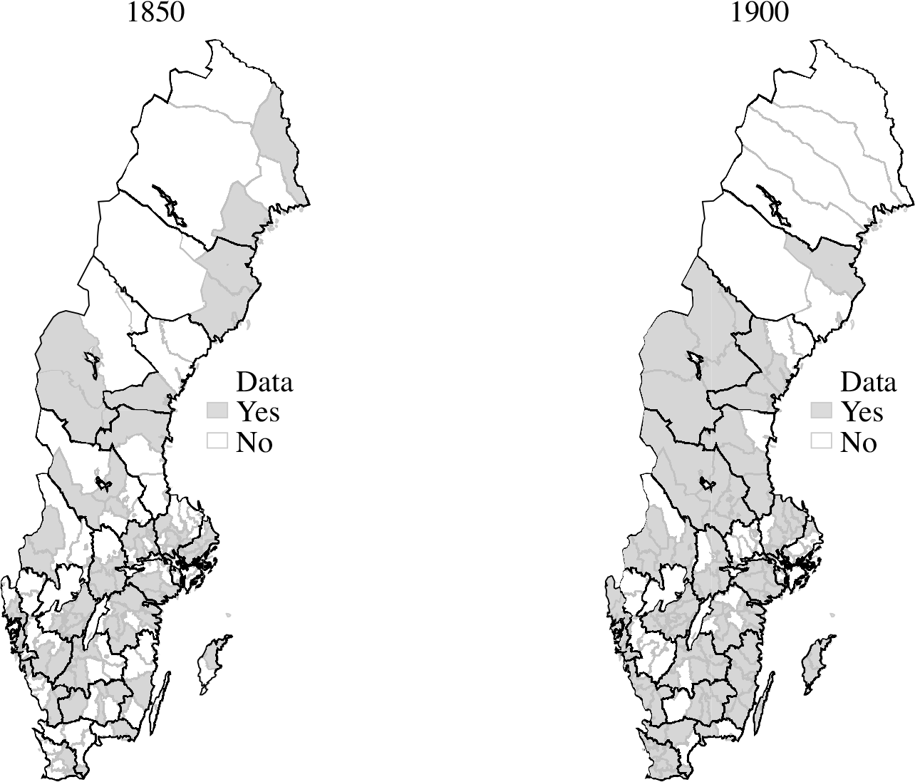
Figure 1 MAP WITH GEOGRAPHICAL DISTRIBUTION OF OBSERVATIONS IN 1850 AND 1900
One possible concern is that wages reported by the bailiwicks and towns might not reflect the going market wages. To check the reliability of our series, we can compare them to existing estimates of wages drawn from other sources. The closest comparison is the series on wages for construction workers hired by municipalities presented by Bagge, Lundberg, and Svennilson (Reference Bagge, Lundberg and Svennilson1935). They collected information from wage rolls in nine Swedish towns between 1875 and 1930.Footnote 4 We have access to data for the same towns for most years over the period up until 1900, allowing us to compare the rates found in our data to those described by Bagge, Lundberg, and Svennilson, which are produced using a different source from ours. A close correspondence would suggest that our wages can be taken as an indicator of the actual going wages rates. In Appendix A, we relate their data to our new series for towns in years when they overlap. It is reassuring that the two series give a very similar picture.
An alternative source of wages is those of day laborers in agriculture collected by Jörberg (Reference Jörberg1972), starting in the eighteenth century. While there could be sectoral wage differences that introduce a wedge between wages of unskilled workers in construction and those in agriculture, a close correspondence of the two series would mean that our wage data can be taken as an indicator of wage rates for groups larger than only construction workers. In Appendix A, we present an additional comparison relating our wages for helpers to those of day workers in agriculture from Jörberg. Our series for rural areas matches the day wages of casual labor in agriculture very closely until the 1880s. After this time, helper wages grow slightly faster, even though the overall pattern of change is very similar.
Hedonic Wage Regression
The problem of incomplete, partial, and changing samples is a challenge to almost all historical wage studies. In our case, the problem results from the fact that the bailiwicks and towns reporting wages are not fixed over time. In addition, some areas did not report wages for all occupations in a certain year (although most did report wages). To confront the challenge of a changing sample, we apply the technique pioneered by Margo (Reference Margo2000) to estimate region- and occupation-specific wages for the antebellum United States. A similar approach was used by Clark (Reference Clark2005) and, more recently, by Gary (Reference Gary2018) and Ridolfi (Reference Ridolfi2019).
The wage regression we estimate is of the following form:
 $$Wag{e_{i,j,t}} = {\beta _1}\;Bailiwic{k_i} + \;{\beta _2}\;Oc{c_j} + {\beta _3}\;Yea{r_t} + {\beta _4}\;\left( {Oc{c_j} \times Yea{r_t}} \right) \\ + {\beta _5}\;\left( {Urban \times Yea{r_t}} \right) + \;{\beta _6}\left( {Oc{c_j} \times Urban} \right) + \;{\varepsilon_{i,j,t}},$$
where Wagei,j,t is the wage in bailiwick i, for occupation j at time t. Bailiwici, Occj, and Yeart are dummies representing each individual bailiwick, the four occupational categories (helper, carpenter, mason, and teamster), and the 15 benchmark years from 1831 to 1900, respectively. The ensuing two terms, Occj × Yeart and Urban × Yeart, are interactions capturing change over time. The first term estimates how the relative wage for the four occupational categories evolves, while the second term captures changes in the relative wage of urban areas. The final term, Occ × Urban, is an interaction between the dummies indicating occupation and urban/rural status, allowing the return to occupation to vary across rural and urban contexts. εi,j,t is the error term.
This regression specification allows us to account for the fact that bailiwicks come in and out of the sample, making our estimate of wages by occupational group and by urban/rural status independent of the bailiwicks reporting wages in a particular year. The graphs presented below show the applied hedonic wage regression, estimating wages while keeping the distribution of bailiwicks constant over the entire period from 1831 through 1900.Footnote 5
Establishing Welfare Ratios
To establish changes in the standard of living of the workers covered in our sample, we follow Allen (Reference Allen2001) in calculating welfare ratios. The method compares wages of workers to the cost of purchasing a basket of goods and allows for a comparison across countries in the number of baskets that a worker was able to afford. Allen provides two baskets: one that represents the level of consumption needed for subsistence and one that reflects the consumption patterns needed to reach a “respectability level” of upkeep.
There is now a lively debate about the assumptions underlying Allen’s calculations. Especially contested are his assumptions about the number of days worked per year, as well as the contribution of different family members to household income (Stephenson Reference Stephenson2018a, Reference Stephenson2018b; Humphries Reference Humphries2013; Humphries and Weisdorf Reference Humphries and Weisdorf2019; Gary Reference Gary2018). While these criticisms are highly relevant for the interpretation of absolute living standards, it is not yet clear what implications they have for comparisons of wage levels, since hitherto these assumptions have been the same across countries. In the absence of comparative work on how to correct these assumptions for individual countries, we use Allen’s data to chart real wages of unskilled workers in European capitals and we apply the same method to our calculation of welfare ratios for Sweden.
To calculate welfare ratios, we have constructed a respectability basket for each of the 24 Swedish counties in each of our benchmark years over the 1831–1900 period. We follow the work of Gary (Reference Gary2018), who has calculated respectability baskets for the three Swedish cities of Stockholm, Malmö, and Kalmar over the 1500–1914 period. We use the same composition of the basket and source for the information on prices as Gary. With one exception, the basket includes the same goods as the respectability baskets for Northern Europe, as calculated by Allen. Gary makes an adjustment for the higher consumption of fish in Scandinavia by assuming a 13 kg consumption of meat and 13 kg of salted fish, instead of the 26 kg of meat assumed by Allen. We follow Gary in this change, but we have also checked the sensitivity to the inclusion of fish instead of meat, and it turns out that it does not affect our results to any significant extent.Footnote 6
The price notations are from Jörberg (Reference Jörberg1972), who collected market price scales for a range of goods over the period from 1732 to 1914. Prices are presented for each county, and for the nineteenth century, the price material is significantly more complete than for earlier periods, both in the coverage of different regions and the type of goods represented. Appendix B details the products used for the different basket items. Information on the regional price of a respectability basket allows us to calculate local welfare ratios. Our regional estimates of the price of a respectability basket follow very closely the pattern over time observed in Gary’s series.
Using our new set of price estimates, we calculate welfare ratios for each bailiwick and town in our sample by deflating the nominal wage with the price of the respectability basket in the county that year. We present mean wages calculated using the hedonic wage regression. We also plot the 25th–75th and the 10th–90th percentile ranges of real wages across bailiwicks and towns. Plotting the distribution allows for a comparison of how the general level of wages developed while also showing how the levels developed at the top and the bottom. This approach also makes it possible to see how the range of local Swedish wages compared to wages in other places.
DID WORKERS BENEFIT FROM ECONOMIC CHANGE? REAL WAGES BY OCCUPATION
In this section, we track the evolution of real wages for our four categories of workers—helpers, carpenters, masons, and teamsters—between 1831 and 1900. During these years, the Swedish economy witnessed radical changes. At the start of the period, the transformation of agriculture produced an increasing number of landless workers. This was followed by early industrialization, taking off in the 1860s. These changes resulted in a growth of real GDP per capita by 120 percent over the period. How was this reflected in the wages of the working class?
Figure 2 shows the development of real wages, measured as the number of respectability baskets that a worker could afford, for each of the four groups of workers. The underlying series are available in Table OA1 of the Online Appendix. In addition to plotting the typical wage, the figure also shows the 25th–75th percentile (dark gray) and the 10th–90th percentile (light gray) ranges of local real wages. It is evident from the figure that real wages were stable or increased slowly for all four groups of workers prior to the mid-1850s, and there is little indication of declining rates. For carpenters, wages grew by 25 percent, while the other groups saw an increase of about 15 percent over the 1831–1855 period. Except for the drop in the mid-1850s, which coincided with an agricultural crisis and rising consumer prices, wages remained stable, with only small variations on a year-to-year basis.
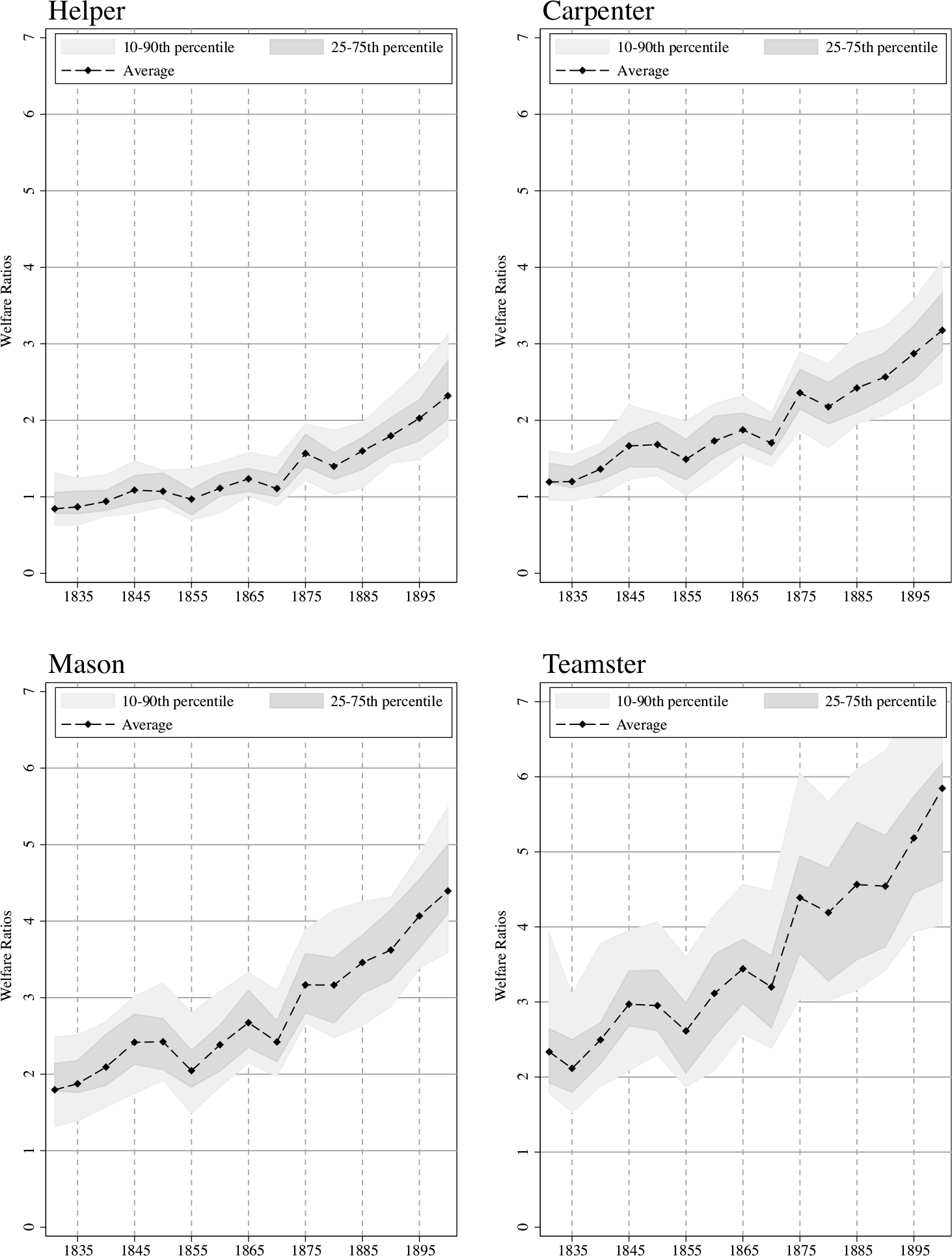
Figure 2 WELFARE RATIOS FOR HELPERS, CARPENTERS, MASONS, AND TEAMSTERS, 1831–1900
What the new series also highlights is the timing of the transition to continuous real wage growth. For the group of workers tracked in these data, this shift appears to have taken place from the mid-1850s onward. Between 1855 and 1900, real wages grew at roughly 2 percent per year, leading to a growth by 140 percent over these 45 years.
The fact that real wages did not deteriorate in the period prior to the 1850s speaks against a pessimistic interpretation of the consequence of the agrarian revolution for the working class. It appears as if increased specialization in agriculture and the growth of the landless did not push down the living standards of unskilled workers. Even in the places with the lowest wages, there is no indication of a tendency for welfare ratios to fall. Our new data also highlight how the evolution of real wages entered a new phase beginning in the mid-1850s. From this point, real wages grew continuously for all four groups of workers. The radical economic shifts that characterized the nineteenth-century Swedish economy appear to have lifted the working class overall. But what were the distributional consequences of these changes?
A straightforward indicator of the relative standard of unskilled workers is the gap in wages relative to more skilled groups such as carpenters and masons. If the labor market position of unskilled workers worsened as the proletariat expanded, we should expect the wage of helpers to decline relative to these more skilled workers. The evidence presented in Figure 2 tells a different story, however. Before the 1850s, unskilled helpers earned just below the amount needed to afford one respectability basket. The corresponding figure was roughly 1.3 for carpenters and two for masons. Between 1855 and 1900, wage premiums decreased from 54 to 37 percent for carpenters and from 110 to 89 percent for masons.Footnote 7 Growing real incomes were accompanied by an increase in the standing of unskilled helpers relative to more skilled workers.
While relative wages for helpers were not negatively affected, the working class as a whole could have lost out, as gains from increased agricultural productivity fell disproportionally into the hands of landowners or as economic growth benefited capitalists and the middle class. This is the mechanism of increased inequality discussed by Lewis. To examine how economic growth was distributed between workers, on the one hand, and the groups of higher social standing, on the other, Figure 3 plots the development of nominal wages for helpers compared to GDP per capita over the same 1831–1900 period. This measure is sometimes called the Williamson index.
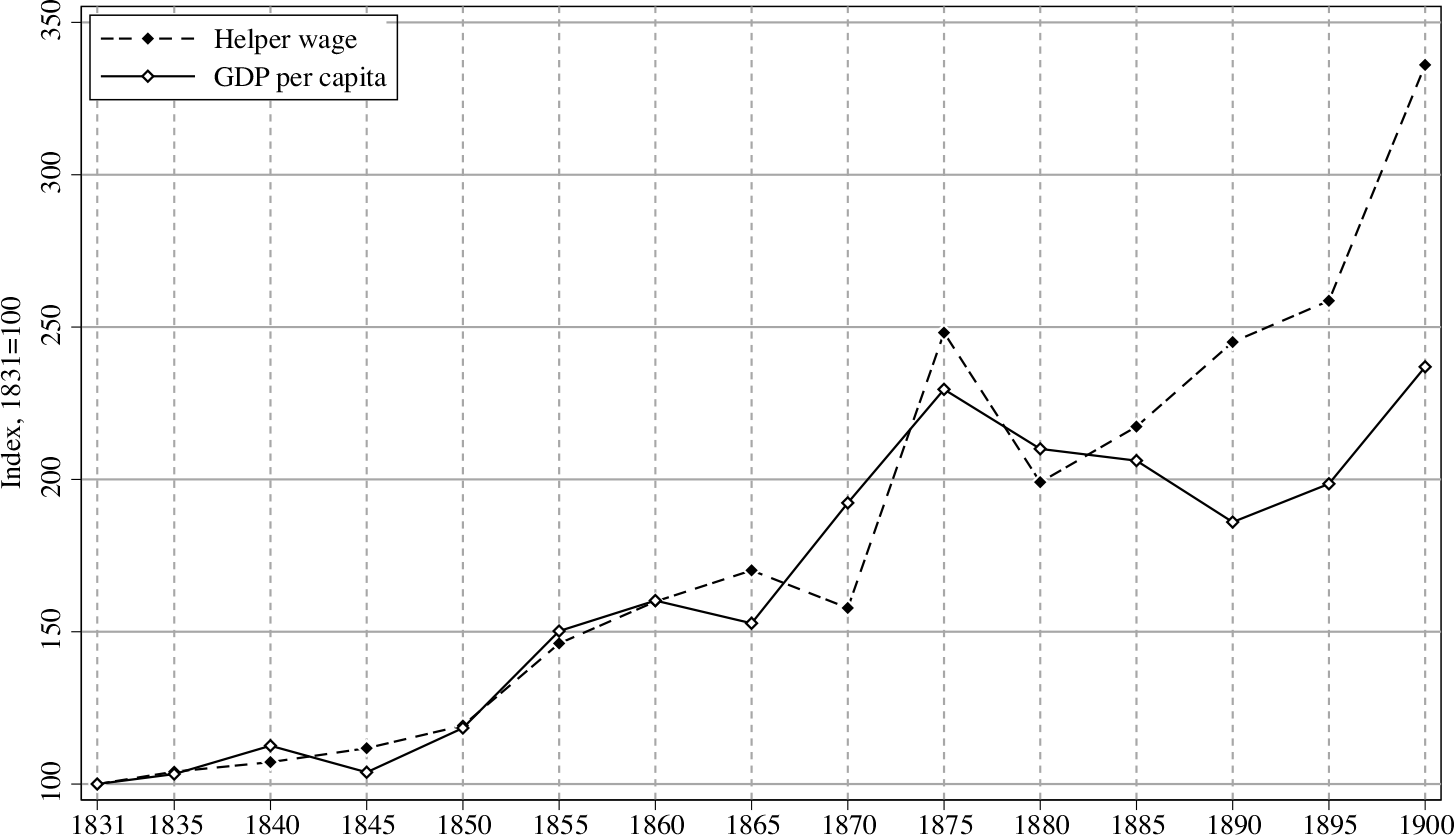
Figure 3 INDEX OF NOMINAL WAGES FOR HELPERS AND NOMINAL GDP PER CAPITA, 1831–1900, WITH 1831 = 100
Focusing first on the period before 1855, it appears that changes in unskilled workers’ wages closely followed the evolution of the economy’s productive capacity. Between 1831 and 1855, nominal wages and GDP per capita both grew by about 50 percent. This suggests that yeoman farmers were not the sole beneficiaries of increasing agricultural productivity during the agrarian transformation and that the growing group of landless wage workers were able to lay claim to a proportionate share of growing incomes.
While real wages were on an upward trend, the transition to continuous wage growth from the 1850s began with large swings in wages and GDP, as seen in Figure 2. The comparison of nominal wages to average income in Figure 3 highlights this even more clearly. The economic crisis of the late 1870s ended the economic boom that had been building in the 1860s and 1870s. Wages of unskilled workers grew in excess of GDP per capita during the economic peak in the mid-1870s, but declined more than the economy after the crisis descended in the late 1870s. This was followed by a catch-up in the middle of the ensuing decade, followed by slightly slower growth during the crisis that followed. From the 1880s, there is a pronounced shift in the behavior of wages. From this time, nominal wages grew much more rapidly than the economy, so much so that, by 1900, nominal wages were more than 225 percent of their 1831 level, while nominal GDP per capita at the same time had grown less than 150 percent. Since the growth of GDP per capita reflects the increase in incomes of all groups, including yeoman farmers, capital owners, white-collar workers, as well as skilled and unskilled workers, the fact that wages for unskilled workers grew faster than incomes for the average person suggests that the income gap between those dependent on wage labor for their living and those of higher social class declined over the course of Swedish industrialization.Footnote 8
These patterns stand in stark contrast to the process described by Lewis. In his model, surplus labor pushes down wages of unskilled workers so that the benefits of economic growth accrue to capital owners and the middle class. In Sweden’s economic transition, we see the opposite. Unskilled wages tracked the growth in nominal GDP per capita before the 1880s and forged ahead after that. This clearly contrasts the experience of Britain and the United States, where real wages of laborers grew more slowly than average incomes, or even stagnated. In the next section, we take a closer look at this process through a comparison of the real wages of unskilled laborers to comparative GDP per capita levels in Sweden and Northwestern Europe.
A Comparison with Northwestern Europe
The collection of real wages for construction workers by Allen (Reference Allen2001) makes it possible to compare our wage series with a number of other locations. We focus the comparison on London, Amsterdam, Antwerp, and Paris. These cities had the highest wages of those in Allen’s database during the nineteenth century, substantially higher than in Southern and Eastern Europe (e.g., Federico, Nuvolari, and Vasta Reference Federico, Nuvolari and Vasta2019). We begin by using respectability baskets to plot welfare ratios of unskilled helpers in Sweden and compare them with the corresponding rates in London and Amsterdam using data from Allen (Reference Allen2001). The results are shown in the left-hand graph in Figure 4. For Sweden, the graph gives the average welfare ratio alongside the 10th–90th percentile of real wages (shown in light gray).
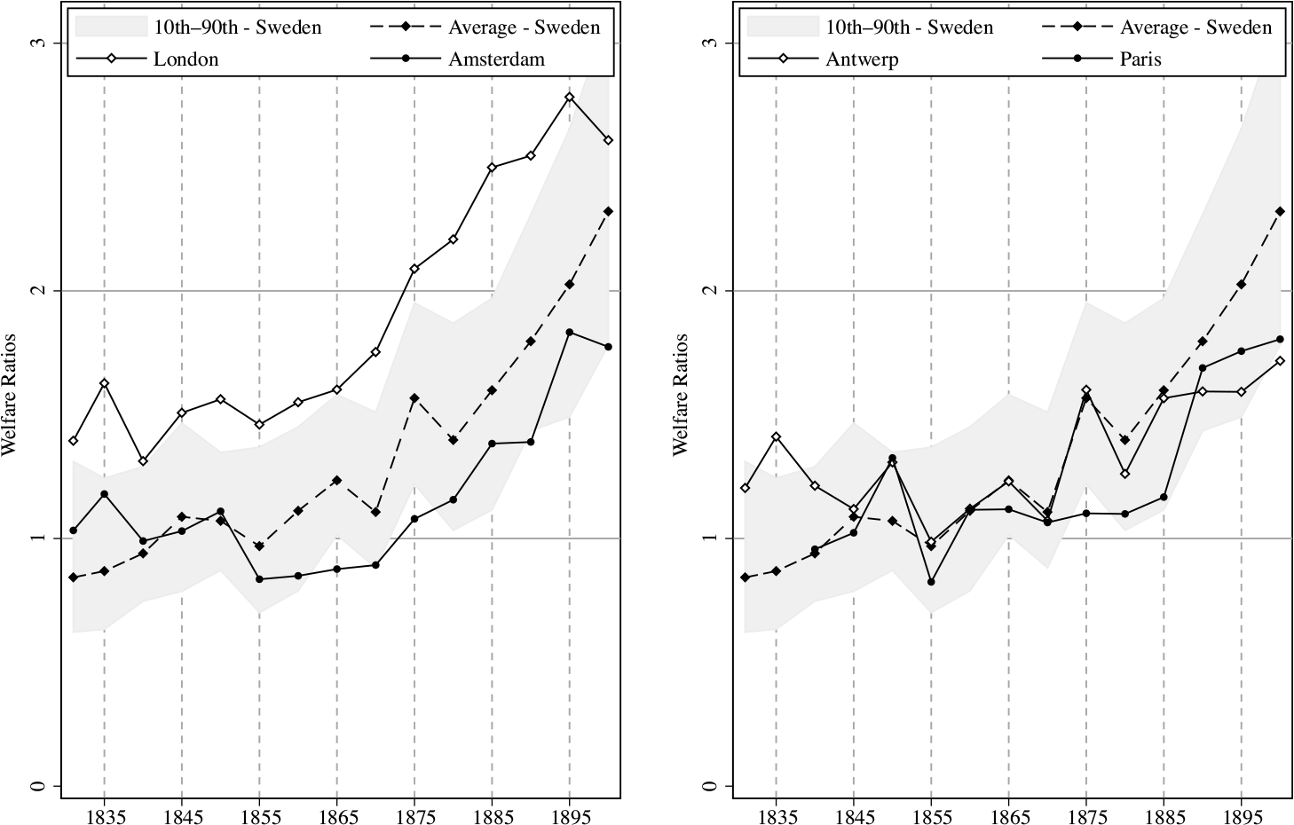
Figure 4 COMPARISON OF REAL WAGES FOR UNSKILLED LABORERS IN SWEDEN, LONDON, AMSTERDAM, ANTWERP, AND PARIS
The graph shows Sweden lagging the two capitals at the start of the period, with average wages below those in London and Amsterdam. Most Swedish laborers earned around 90 percent of the amount needed to purchase a respectability basket for a family in the 1830s and 1840s. The corresponding rate in Amsterdam was around 1, while London was ahead with 1.5. However, the 10th–90th percentile range of wages shows that some places in Sweden already had higher wages than those in Amsterdam in the 1830s and 1840s. Mean Swedish wages overtook those of Amsterdam from the 1860s onward. Except for the period during which there was a sharp fall in wages in the early 1880s, Swedish wages were about 20 percent higher than wages in the Dutch capital throughout the late nineteenth century. Wages of unskilled workers in Sweden were also catching up with those in London as the British advantage fell from around 80 percent in the 1850s to about 40 percent by the 1890s. The range also shows how even the 10th percentile of Swedish real wages was on par with the wages in Amsterdam in 1900, and wages at the 90th percentile of our Swedish sample were above those in London at the same point in time.
The right-hand graph in Figure 4 extends the comparison to Antwerp and Paris. The figure shows Swedish wages outgrowing those in Paris around the same time as those in Amsterdam and remaining higher than in the French capital throughout the rest of the nineteenth century. For Antwerp, the largest city in one of the leading industrial economies at the time, wages were growing at a faster pace than in Amsterdam and Paris. In this case, Swedish wages followed the level in Antwerp from about 1860 and eventually outgrew them from 1885 onward. By 1900, real wages at the 10th percentile of the Swedish sample were on par with those in Antwerp and Paris, suggesting a substantial Swedish overall advantage.
The growth of Swedish wages is impressive seen in this comparative light. Only London had higher levels by the end of the nineteenth century. The lowest wages in Sweden were at the level of those in Amsterdam, Antwerp, and Paris, and the highest were higher than wages in London. This implies that unskilled workers in Sweden were among those with the highest comparative living standard in the nineteenth century; wage rates in the capitals of Southern and Eastern Europe, as well as in other parts of the world, were substantially lower than those in the cities compared in Figure 4.
One possible explanation for the high Swedish wages could be the fast growth of the Swedish economy in the latter half of the nineteenth century. To examine the role economic progression played in expanding real wages, it is necessary to put the welfare ratios presented previously into the context of levels of GDP per capita. In Figure 5, we plot welfare ratios on the Y-axis, just as in Figure 4, and on the X-axis, we show the comparative level of GDP per capita in Sweden, Britain, and the Netherlands, respectively, taken from the latest release from the Maddison Project (Bolt and Van Zanden Reference Bolt and van Zanden2014). Just as in the previous figure, the light-gray area shows the range of the 10th–90th percentile of real wages in the Swedish data.
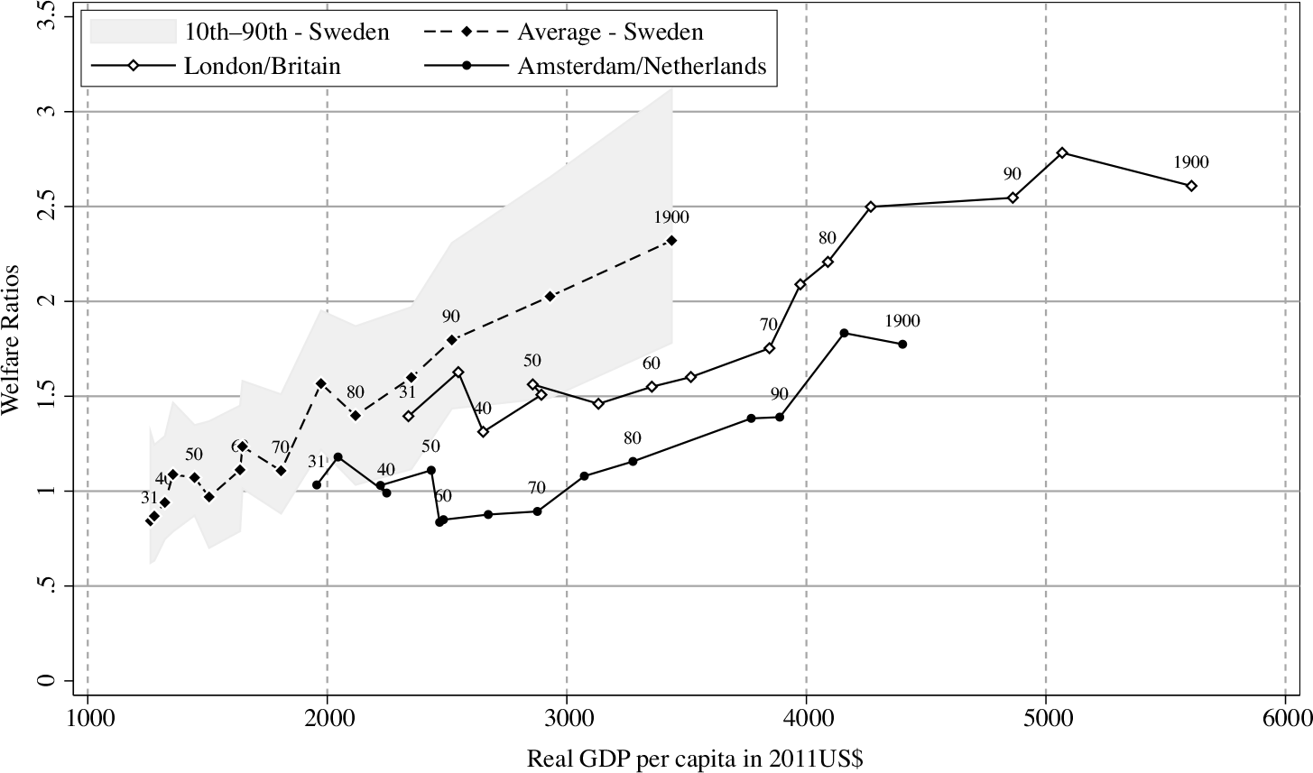
Figure 5 PLOT OF REAL WAGES FOR UNSKILLED LABORERS AND GDP PER CAPITA IN SWEDEN, LONDON/BRITAIN, AND AMSTERDAM/NETHERLANDS
The figure shows that the spurt in Swedish wages was not simply the result of a rapidly growing economy. In 1880, when Swedish per capita income levels were at the level that the Netherlands had attained by 1840, wages were higher in the Swedish case. The same is true in comparison to Britain. While Britain had the same level of GDP per capita in 1831 as Sweden in 1885, the welfare ratios of unskilled workers were higher in Sweden than in London at the same level of per capita income. The range of Swedish wages also shows that the areas with the lowest wages did comparatively well.
The patterns of real wages over the path of development are very revealing. Consider the period when the three countries grew from GDP per capita levels of 2,000 USD (in 2011 levels) to about 3,500. In Sweden, this happened between 1880 and 1900, whereas in Britain, this occurred before 1865 and in the Netherlands, between 1831 and 1880. Over the course of this transition, Swedish welfare ratios grew from around 1.5 to just below 2.5. In Britain and in the Netherlands, by contrast, ratios remained mostly stable at 1.5 in the case of Britain and at around one in the Dutch case.
Figure 6 extends the comparison to Antwerp and Paris. The same pattern that appeared in the comparison with London and Amsterdam also appears here. At a given level of GDP per capita, Swedish wages were higher than those in Antwerp and Paris. Between GDP per capita levels of 2,000 and 3,000 USD, wages remained mostly stagnant in Paris and Antwerp, while for Swedish workers, they almost doubled.
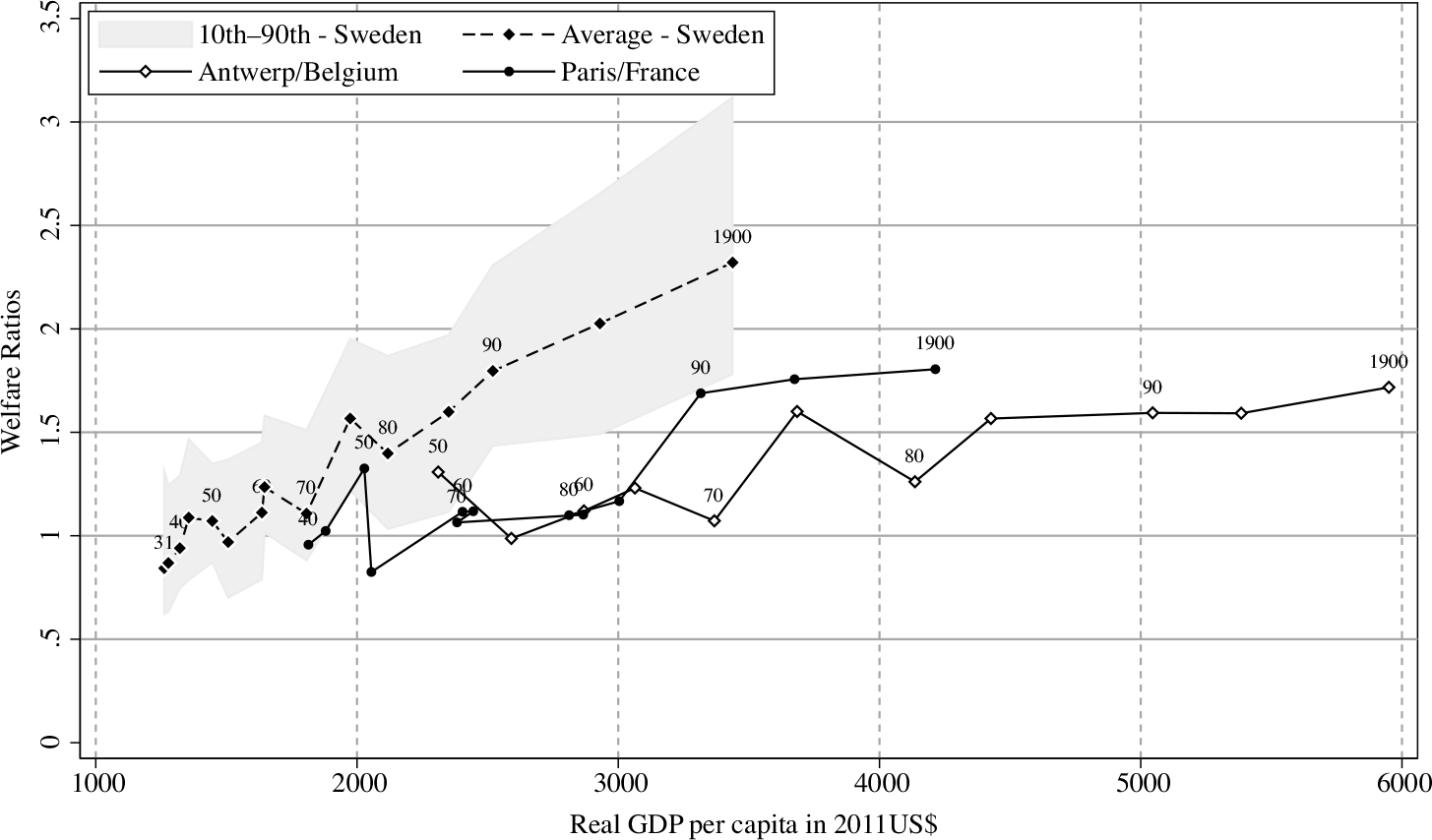
Figure 6 PLOT OF REAL WAGES FOR UNSKILLED LABORERS AND GDP PER CAPITA IN SWEDEN, ANTWERP/BELGIUM, AND PARIS/FRANCE
It appears that stagnating real wages were indeed a feature of economic growth in the leading countries in Europe at the time of their industrialization. However, Sweden clearly breaks away from this pattern. Here, wages of unskilled workers continued to grow throughout the process of early industrialization. The absolute level of wages was also higher. For a given level of GDP per capita, Swedish workers could afford about a basket more of respectability goods than workers in the major capitals of Europe. The range of wages also reveals that even in the places at the 10th percentile of the Swedish distribution, wages were comparatively high.
Our results conform with findings from the literature on human heights. Sweden had the tallest population in Western Europe throughout the nineteenth century, and height increased continuously throughout the century (Baten and Blum Reference Baten and Blum2014; Öberg Reference Öberg2014), which is in line with Baten’s (Reference Baten2000) finding that height is more closely related to wages than to GDP per capita.
It should also be noted that our results are not driven by the fact that we compare Sweden as a whole to capital cities. If we compared instead to welfare ratios in Stockholm, the Swedish advantage would appear even starker. Throughout the period, real wages in Stockholm were about 50 percent higher than those in the rest of the country and the growth in wages was faster: about 190 percent compared to 175 percent for the country as a whole.Footnote 9
Another worry could be that our wages are not representative of the experience of unskilled workers more broadly. Arguing against this is the fact that our series for rural helpers closely follows the existing evidence for day rates in agriculture and wages for unskilled workers in manufacturing were even higher than the rates we use (Lundh and Prado Reference Lundh and Prado2015). In the following section, we explore some of the causes of this impressive development of real wages.
WHY DID SWEDISH WORKERS BENEFIT SO MUCH FROM ECONOMIC GROWTH?
The evidence presented in the previous section shows that Swedish workers benefited to a much greater extent from economic growth than did workers in other places. In this section, we investigate some of the factors that could explain why Swedish laborers were able to reap the benefits of the economic transformation to such a great extent. We do this in four steps. We start by looking at the role played by price changes. The nineteenth century was a period of rapid globalization, and falling prices for foodstuffs could be a cause of rising wages. Next, we look at the size of the urban-rural wage gap. If economic development took place without forcing a wage gap between urban and rural places, this could be one reason average wages grew so quickly. Third, we analyze regional wage convergence. High rates of convergence would suggest that workers were willing and able to move to places with higher real wages. Strong convergence would then push up wages in areas with lower wages and contribute to growing wages. Fourth, we consider the impact of overseas migration. By reducing the supply of labor, mass migration to the New World could have had a positive effect on wages.
The Role of Price Changes versus Nominal Wage Increases
We follow Federico, Nuvolari, and Vasta (Reference Federico, Nuvolari and Vasta2019) in considering the relative contribution of wage and price changes to the resulting change in welfare ratios. During the nineteenth century, rapid globalization led to a convergence in prices across the world. The most dramatic impact came from the “Grain Invasion,” when grain produced on the agricultural plains of the American Midwest began to flood Europe and put a downward pressure on the price of foodstuffs. This development benefited the working class (O’Rourke Reference O’Rourke1997), and some of the growth in real wages, therefore, could be the result of price changes rather than increases in nominal wages.
To examine the role of price changes and nominal wage increases, we compare the trajectory of the actual real wage compared to two counterfactuals. In the first counterfactual, we hold nominal wages fixed at their level in 1831 and allow the price of the basket of goods to vary over time as it did. In the second counterfactual, we instead hold the price of the basket fixed at the level it was in 1831 but let nominal wages grow as they did. The resulting series are shown in Figure 7.
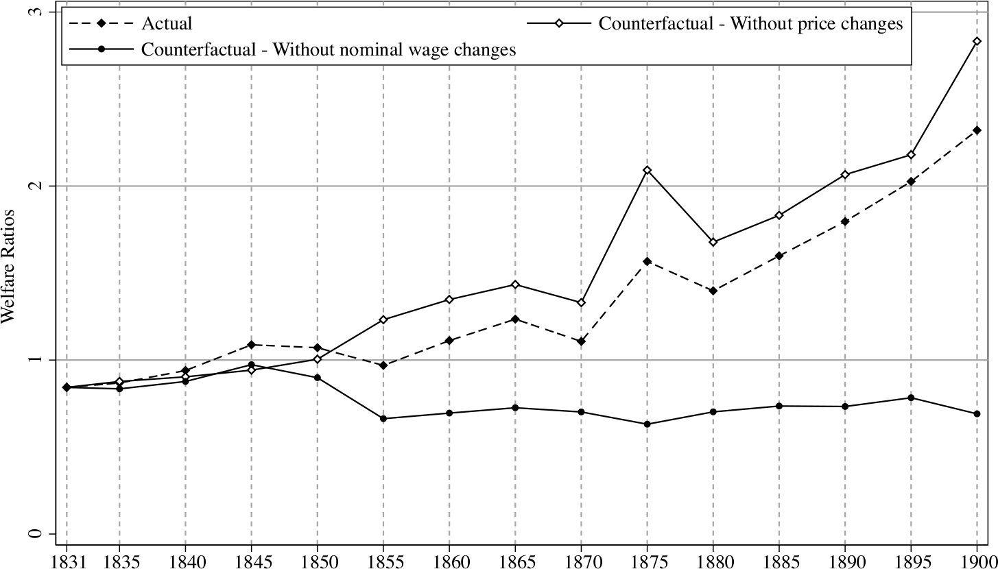
Figure 7 ACTUAL AND COUNTERFACTUAL REAL WAGES FOR HELPERS, 1831–1900
This figure shows that most of the growth in real wages over the 1831–1900 period was the result of nominal wage increases rather than price changes. Prices fell slightly in the 1830s and 1840s and then rose sharply in the early 1850s. From that point onward, living costs remained stable, showing only a brief uptick in the early 1870s and then a declining tendency throughout the 1880s and 1890s, resulting in a slight increase in the price of a respectability basket over the full period. As shown in Figure 7, in the absence of nominal wage increases, the welfare ratio would have declined from about 0.8 to just under 0.7. As a corollary, if living costs had remained at their 1831 level, real wages would have increased even more than they did. The welfare ratio would have grown from 0.8 to just above 2.8 instead of to around 2.3, which was actually the case.
This counterfactual calculation suggests that while external factors such as globalization and the grain invasion put a check on the increase in the prices of foodstuffs, they were not decisive factors for the trajectory of real wages.
Urban-Rural Differentials
In this section, we compare the wages of workers in urban and rural areas. Our new data set allows us to look at similar workers in different localities. This is a substantial improvement over previous studies on the Swedish urban wage premium, as these have relied on comparisons of manufacturing workers to day workers in agriculture. Our data also covers a much larger set of towns than any previous data set. If economic development took place without forcing a wage gap between urban and rural places, then that could possibly explain why average wages grew so quickly. This is most relevant for the later part of the nineteenth century, when urban areas began to play a more prominent role in the process of industrialization (Lundmark and Malmberg Reference Lundmark and Malmberg1988).
In Figure 8, we plot the evolution of nominal wages for helpers in urban and rural areas. The resulting series, given in the figure, suggests a small gap throughout the period from 1831 to 1900; the differential never rose above 10 percent after the 1830s. While there was a slight increase in the gap with the onset of real wage growth from 1855, it is clear that both urban and rural areas followed in the transition to growth. Toward the end of the period, rural areas caught up and, in 1900, even superseded their urban counterparts.Footnote 10

Figure 8 NOMINAL WAGES FOR HELPERS IN RURAL AND URBAN PLACES, 1831–1900
If we look at the urban-rural gap for the other occupations, we find a pattern very similar to the one for helpers: The gap was smaller for carpenters, while it was slightly larger for masons and teamsters. For no occupation did the gap exceed 20 percent at any point after the 1830s.Footnote 11
Figure 8 refers to nominal wages. Unfortunately, there are no existing data series of rural and urban costs of living in Sweden over this period.Footnote 12 Allen (Reference Allen1955) provides estimates for 1870 and 1900. His results suggest that the increase in monetary income needed for an agricultural worker to transfer to the industrial sector with maintained real income was about 7 percent in 1870 and 6.5 percent in 1900. The results are dependent on assumptions about consumption patterns and some backward extrapolation of prices and, therefore, should be interpreted with care. What evidence there is, thus, suggests that even though the difference in the cost of living was not very large, if we account for the disparity in prices between rural and urban areas, the real gap in wages largely disappears.
Other factors are likely to have affected the compensating wage differential between rural and urban areas, as well. Mortality was higher in cities, even though the difference declined over time: from 1.61 in the 1871–1880 period to 1.24 by the 1891–1900 period (Lundh and Prado Reference Lundh and Prado2015). Selective migration to cities is also likely a factor that caused higher wages there. While it is difficult to assess whether urban migrants were positively selected on unobservable characteristics, such as innate ability, available evidence indicates that migrants to cities came disproportionally from higher-status households (Eriksson Reference Eriksson2015).
Given the small or nonexistent urban real wage premium, the evidence for mortality and selection alone would suggest that urban real living standards were lower than in the countryside. However, there were other factors that held up daily wages in rural relative to urban areas that need to be taken into account. Employment was more stable over the year in towns, and jobs were also more readily available, meaning that search and matching costs were lower. For individuals working for day wages, this would translate into higher yearly incomes, and workers in rural areas would have to have been compensated for this by higher daily wages. In 1913, the first year for which we can compare both daily and yearly wages of manufacturing and tertiary workers to those in agriculture using the official statistics, the ratio between the two sectors was much lower in terms of daily wages than in terms of yearly enumeration, suggesting that urban workers were better able to translate their daily wages into yearly income.Footnote 13
One concern could be that our definition of cities is based on administrative boundaries rather than population size. Since many cities were, in fact, not very large, our results could possibly reflect our choice of definition rather than a small urban-rural wage gap. To account for this, we compare the eight largest cities with their surrounding counties. These series are presented in Figure OA1 in the Online Appendix. The results show that in almost all cases, wages in the neighboring countryside followed closely those in the city.
It is not so surprising that wages in cities did not greatly exceed those in rural areas during the early part of Sweden’s industrialization. Before the late nineteenth century, most expanding industries were located in the countryside, in proximity to natural resources and water power (Gårdlund Reference Gårdlund1942; Berger, Enflo, and Henning Reference Berger, Enflo and Henning2012). It is more extraordinary that differentials remained small even as urbanization began to play a more prominent role from the late nineteenth century onward. From this point forward, expanding employment opportunities in urban areas meant that they were able to attract a large number of internal migrants from rural areas and employment was able to expand in urban areas without a large differential in wages (for migration rates, see Table 3 in Lundh and Prado Reference Lundh and Prado2015).
Regional Convergence
While industries sprung up predominantly in the countryside, the process of industrialization spread unevenly across the country. Without well-integrated labor markets, this process would have resulted in increasing differences in wages across regions. Convergence in real wages across different parts of the country would also mean faster growth in average wages than would have been the case otherwise and could help explain why Swedish wages grew so fast.
To keep the regional units fixed over time for the analysis of convergence, we create a panel for each occupation with one wage observation per county, per year. To arrive at occupation-specific county wages, we take the median of the wage observations from the county in that observation year. We start the panel in 1840, when we have a larger sample that allows us to calculate county medians. We do not have data for Gotland county (an island in the Baltic sea) in 1840 and 1860 or for the Northern counties of Jämtland and Västerbotten in 1865 and 1845, respectively. Apart from those gaps, we have a full panel of 24 counties over the 1840–1900 period. We divide the resulting estimate of nominal wages in each county by the cost of a respectability basket in the same county to arrive at regional welfare ratios.
To consider convergence formally, we estimate the unconditional rate of convergence using the following model:
 $$
{1 \over T}\ln {{{W_{i,t + 1}}} \over {{W_{i,t}}}} = x + \gamma \;{\rm{ln}}\left( {{W_{i,t}}} \right) + {\varepsilon _{i,t}},$$
$$
{1 \over T}\ln {{{W_{i,t + 1}}} \over {{W_{i,t}}}} = x + \gamma \;{\rm{ln}}\left( {{W_{i,t}}} \right) + {\varepsilon _{i,t}},$$
where T is the number of years and W is the welfare ratio in year t for county i. We estimate the equation using regular ordinary least squares regression. In addition to unconditional convergence, we also estimate the level of conditional convergence using county-fixed effects. Following Rosés and Sánchez-Alonso (Reference Rosés and Sánchez-Alonso2004), the implied yearly rate of convergence can be derived from the above equation using the following formula:  $\beta = - \left( {1/T} \right){\rm{ln}}\left( {\gamma T + 1} \right)$. The results for all groups are shown graphically in Figure 10. The full table of regression results for all occupations pooled together, as well as for each worker category individually, is available in Table OA3 in the Online Appendix.

Figure 9 UNCONDITIONAL AND CONDITIONAL CONVERGENCE OF REAL WAGES
The results indicate that there was substantial convergence in real wages for all four occupations and all point estimates are statistically significant at the 1 percent level. Estimated convergence rates differ somewhat across occupations, but they all suggest a strong tendency for the lowest wages to grow more rapidly than the average over the subsequent period. For the regression with the four occupations pooled together, which is also shown graphically in Figure 9, the implied rate of unconditional convergence is 8.5 percent and the corresponding rate for conditional convergence is 11.8 percent. For comparison, O’Rourke and Williamson (1997) estimate an unconditional convergence rate of 3.3 percent for a set of Old and New World countries between 1870 and 1913.
We also examine whether convergence rates differed across time periods. This allows us to inspect whether the pulling together of labor markets was something that appeared because of industrialization or if convergence was already well underway prior to this. We do this by comparing convergence coefficients for each five-year period over the 1840–1900 period. The full table of regression results is provided in Table AO4 in the Online Appendix. Interestingly, the estimated rates of convergence are very similar across time. The fact that convergence was present so early suggests that labor markets were also integrating before the economic takeoff in the 1860s.
Our results line up with previous research on Swedish spatial development. Collin (Reference Collin2016) finds an implied unconditional convergence rate of 4.4 percent for real wages in manufacturing over the 1860/64–1912 period, while it was 3.1 percent for agricultural workers over the 1872–1913 period (see also Collin, Lundh, and Prado Reference Collin, Lundh and Prado2018). Our higher rate could be explained by the difference in period and the occupations covered, but as a whole, these results suggest a strong rate of regional convergence of real wages across the nineteenth century, regardless of economic sectors and data sets.
The results for wages also conform to the pattern for regional GDP per capita estimated by Enflo, Henning, and Schön (Reference Enflo, Henning and Schön2014), indicating strong convergence between the 1860s and WWI. Enflo and Rosés (Reference Enflo and Rosés2015) compare the dispersion of regional GDP per capita and show that Swedish convergence was so strong that, by the 1910s, the country had the lowest dispersion of all countries with comparable data.
What could account for this level of labor market integration? Enflo, Lundh, and Prado (Reference Enflo, Lundh and Prado2014) show that internal migration was very responsive to wage differentials and shifted supply away from low wage regions, acting as a catalyst for wage growth in those places.Footnote 14 In a similar vein, Söderberg (Reference Söderberg1985) examined the responsiveness of internal migration to regional dispersion in wages and showed—in a comparison with France, Britain, and Prussia—that Sweden displayed the highest receptiveness. These results indicate that responsiveness to changed market conditions could help explain the pattern of rapid wage growth.
Overseas Migration
An additional factor that could assist in explaining the fast growth of Swedish real wages is overseas migration, as it likely reduced the supply of labor and strengthened the position of unskilled workers. Between 1851 and 1900, more than 840,000 Swedes migrated to the United States, and Sweden had one of the highest emigration rates of any country in the late nineteenth century (O’Rourke and Williamson Reference O’Rourke and Williamson1999). Enflo, Lundh, and Prado (Reference Enflo, Lundh and Prado2014) and Karadja and Prawitz (Reference Karadja and Prawitz2019) argue convincingly that places within Sweden with more emigration to the New World also experienced more rapid growth of unskilled workers’ wages (see also Ljungberg Reference Ljungberg1997; O’Rourke and Williamson Reference O’Rourke and Williamson1995). Their respective analyses underline the endogeneity of migration with respect to real wage growth. This results from the fact that places with faster wage growth were also likely to experience less emigration (see the results in the work of Bohlin and Eurenius Reference Bohlin and Eurenius2010), and these authors take great care to avoid these endogeneity problems by instrumenting for migration.
Keeping this important caveat in mind, Figure 10 shows the correlation between ten-year net-overseas migration rates and real wage growth, as well as the growth of wages for helpers relative to carpenters, masons, and teamsters over the same span of time, using our data on wages.Footnote 15 We are the first to analyze relative wage growth for unskilled workers. The figure suggests a correlation both for real wage growth and relative wage growth that is statistically significant at the 1 percent level. The estimate for real wage growth suggests that a county experiencing a net-overseas migration rate at the median of the sample (−2.5 per thousand people) would see an extra 22 percent growth in real wages over the period from 1831 to 1900. This effect was even more pronounced in the counties of Jönköping, Kronoberg, Halland, and Värmland, which had the highest emigration rates and where net-overseas migration averaged about −4.5 per thousand people. In these counties, the effect on real wage growth would have accumulated to about 40 percent over the period. The right-hand panel also shows how overseas migration was correlated with stronger growth in the wages of helpers relative to the more skilled groups of carpenters, masons, and teamsters. A county with median overseas migration rates experienced a 14-percentage-point growth in unskilled wages over the wage growth for more skilled groups, as compared to a county without a net outflow.

Figure 10 CORRELATION BETWEEN OVERSEAS EMIGRATION AND REAL WAGE GROWTH AND RELATIVE WAGE GROWTH FOR HELPERS
While these are only correlations, and because of possible endogeneity, these results should be interpreted with care. Together with the more detailed analyses conducted by Enflo, Lundh, and Prado (Reference Enflo, Lundh and Prado2014) and Karadja and Prawitz (Reference Karadja and Prawitz2019), however, they clearly point to emigration as a key factor for Swedish real wage growth in the period. Our results for relative wage growth of unskilled workers also help to explain why industrialization in Sweden coincided with falling skill differentials.Footnote 16
The indicators of labor market flexibility and integration that we have tracked suggest that the Swedish labor market functioned very well in the nineteenth century. Rapid regional convergence and small urban-rural wage gaps indicate that the labor market was quick to adjust to new opportunities that appeared as a result of the economic transformation. This was likely facilitated by the homogeneity of the population in terms of ethnicity and language. On top of this, Sweden experienced a positive influence from emigration to the New World that pushed up wages for workers and helps to explain why industrialization coincided with falling skill differentials. Together, these factors produced rapidly growing real wages and high comparative living standards for the Swedish working class.
CONCLUSIONS
In this paper, we have shown how Swedish workers’ wages grew strongly during the early phases of industrialization, in stark contrast to influential theories as well as the experience of other countries. We used a newly compiled data set that includes wages for helpers, carpenters, masons, and teamsters and has a uniquely detailed geographical coverage, as it encompasses a broad set of places in the countryside as well as a large proportion of towns—the vast majority of which have never been covered before.
We found that real wages were stable or increased slowly prior to the mid-1850s, but grew rapidly thereafter. Examining distributional impacts, we established that workers’ wages tracked the evolution of GDP per capita until the 1880s and outgrew the economy from that point. Our comparison of unskilled wages in Sweden to those of the leading cities of Northern Europe additionally showed that standards of living were higher in Sweden at a given level of GDP per capita. In the Swedish case, economic growth was concurrent with increasing real wages, while for the countries in the comparison, wages were stagnant or grew more slowly.
Swedish laborers benefited from favorable external factors, such as globalization forces and the prospect of mass migration to the United States, combined with well-integrated and flexible labor markets that allowed the working class to reap the benefits of economic growth. This was signified by the lack of surging skill differentials, small urban-rural wage gaps, and strong convergence of real wages across regions.
Other explanations, such as inclusive institutions and strong labor movements, which are sometimes invoked to explain the distribution of economic growth, are less likely (Acemoglu and Robinson Reference Acemoglu and Robinson2000, Reference Acemoglu and Robinson2015; Bengtsson Reference Bengtsson2019). Sweden’s political institutions were very unequal at the time, and since labor unions had not yet evolved, they can hardly be the reason for the development in this case. Neither is it likely that the fertility rate was an important factor, since Sweden’s demographic transition followed the general European trend and experienced declining fertility rates starting only in the late nineteenth century (Bengtsson and Dribe Reference Bengtsson and Dribe2014).
The Swedish case shows how the development of real wages for laborers can deviate significantly from the trajectory of GDP per capita, and we have explored possible reasons why this was the case. The implication is that future studies of comparative living standards should consider both wages and GDP per capita, and when there is a divergence between the two, researchers should take care to analyze possible reasons for the disconnect.
Appendix A: Comparison with Existing Wage Series
In this appendix, we compare existing series of unskilled wages to those in the new data set. We begin with a comparison to the series of wages for unskilled workers in municipal construction presented by Bagge, Lundberg, and Svenilsson (Reference Bagge, Lundberg and Svennilson1935), followed by the data on day wages in agriculture from Jörberg (Reference Jörberg1972).
Comparison to the Bagge, Lundberg, and Svenilsson Series
Bagge, Lundberg, and Svennilson (Reference Bagge, Lundberg and Svennilson1935) have produced wage data series for municipal construction workers in some towns between 1865 and 1930. For the 1875–1890 period, in addition to Stockholm, they present wages for four towns: Helsingborg, Västerås, Visby, and Karlskrona. Our data also cover these four towns during this period. For the 1890–1900 period, the Bagge sample expands and consists of nine towns: Gothenburg, Malmö, Norrköping, Helsingborg, Gävle, Västerås, Sundsvall, Borås, and Karlskrona. Norrköping enters the sample from 1896. Our data cover these towns as well, except for Västerås after 1890.
Figure A1 presents a comparison between our data for helpers and the Bagge data for unskilled workers in the towns that are covered in both data sets. The overall takeaway from the comparison is that the two series follow each other closely. Special attention should be given to the series for Helsingborg, Västerås, and Karlskrona, where there are many years with data from both sources. In those cases, the fit between the series is very close. Overall, the correlation between the two series is 0.92, with an adjusted R-squared of 0.65.

Figure A1 COMPARISON WITH THE BAGGE DATA FOR NINE TOWNS, HOURLY WAGES FROM 1875 TO 1900
Comparison to Jörberg’s Series for Agriculture
Jörberg (Reference Jörberg1972) presents an unweighted average of county day wages in agriculture between 1732 and 1914. The data are drawn from market price scales negotiated in each county and used as administrative prices when assessing the cash value of dues in kind. While this leads to a concern that these are not market prices, Lundh and Prado (Reference Lundh and Prado2015) present a series of wages for unskilled agricultural workers after 1865 based on official statistics, which closely follow the series from Jörberg.
Figure A2 presents a comparison of the Jörberg series to our data for helpers in rural areas. While the two series both refer to rural workers, they relate to different sectors, so there could be industry-specific premiums that create a wedge between wages in the two economic activities. The sources are also different, with our data having a larger quantitative basis and a wider geographical coverage. However, from Figure A2, it appears that the two wage series move very closely together. After 1885, there is some deviation, as wages in agriculture grow more slowly than wages for helpers. However, the overall pattern is very similar. We have also double-checked that our comparisons of wages in Sweden to those in Northern European cities are not significantly affected if we use the series for agricultural workers instead.

Figure A2 COMPARISON WITH JÖRBERG’S SERIES FOR DAY WORKERS IN AGRICULTURE
Appendix B: Regional Cost of Living
In this appendix, we explain the construction of the regional cost-of-living indices we use to calculate welfare ratios. We use the cost of a respectability basket as set out by Allen (Reference Allen2001) and the same basket content and source for the information on prices as Gary (Reference Gary2018), who has calculated the cost of a respectability basket for the three cities of Stockholm, Malmö, and Kalmar over the 1500–1914 period. The prices are drawn from the work of Jörberg (Reference Jörberg1972), who collected market price scales for a range of goods over the period from 1732 to 1914. Prices are presented for each county, and for the nineteenth century, the price material is considerably more complete both in the coverage of different regions and the types of goods represented.
We calculate the cost of a respectability basket for each of the 24 Swedish counties each year. In cases where there is no local price available for a specific good, we have used the price in the closest region with data. After 1875, there is no information in Jörberg’s data on the price of Baltic herring. To extend the series up to 1900, we use the evolution of rye prices, which are strongly correlated with herring prices in the preceding period. We similarly lack data on the price of tallow candles after 1875. We use the evolution of the price for tallow to bring the series for tallow candles up to 1900. Table B1 details the products from Jörberg (Reference Jörberg1972) that we use for each of the components in Allen’s basket, with Gary’s adjustments for the consumption of fish in Sweden.
Table B1 GOODS INCLUDED IN THE CONSTRUCTION OF REGIONAL RESPECTABILITY BASKETS
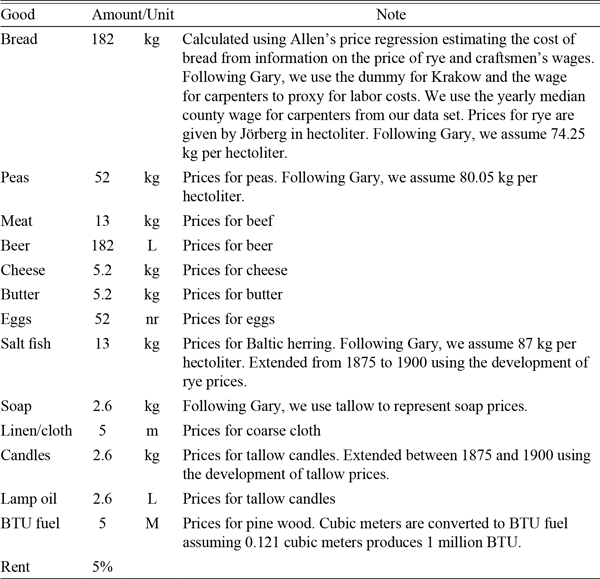
Note: Data on prices are from Jörberg (Reference Jörberg1972). The construction of the basket and the goods and prices included build on the work of Gary (Reference Gary2018).
The resulting series of regional costs of respectability baskets very closely follow the pattern over time in Gary’s series. We have also experimented with replacing fish with meat, as in the original Allen basket, to make sure our results are not driven by this change, and the cost of the basket does not change notably.


 Open access