… many a landlord is deciding that it is better to sell at the inflated market price than to rent at a fixed ceiling price. The ceiling on rents, therefore, means that an increasing fraction of all housing is being put on the market for owner-occupancy, and that rentals are becoming almost impossible to find, at least at the legal rents.
— Milton Friedman and George J. Stigler,
Roofs or Ceilings? (1946)
The mid-twentieth century increase in home ownership in the United States is often framed as a post-World War II change, associated with surging construction of new housing in suburban areas (for example, Jackson Reference Jackson1985). The years from 1945 to 1960 indeed saw home ownership rise rapidly. Yet intercensal survey estimates suggest that the home ownership rate increased by 10 percentage points between 1940 and 1945, slightly more than the postwar rise from 1945 to 1960. The timing of this increase is seemingly incongruous with differences in housing supply between the wartime and postwar periods: in contrast to the high elasticity of postwar construction, residential construction was severely restricted during the war. This article investigates one of the largest government interventions in housing markets during the 1940s—wartime and postwar rent control—and illuminates its role in this “wartime” rise in home ownership.
World War II saw the most widespread imposition of rent control in the history of the United States. Roughly 80 percent of the 1940 rental housing stock lay in areas that the federal government put under rent control between 1941 and 1946. At the same time, sales prices were not controlled. Many observers at the time, including Milton Friedman and George Stigler (Reference Friedman and Stigler1946), argued that rent control led to higher rates of home ownership as landlords chose to sell at uncontrolled prices rather than continuing to rent out their properties at the controlled price. Consistent with this story, a large share of the wartime increase in home ownership came from the same dwellings shifting from renter- to owner-occupancy.Footnote 1 But most contemporary arguments on the importance of rent control were based solely on aggregate national trends, even though many other factors—such as rising income and savings or increasing marginal tax rates—could have played a role in the observed shift in housing tenure.
An empirical test of the hypothesis that wartime rent control increased home ownership is complicated by the fact that nearly all urban areas were placed under rent control during the war. To overcome this challenge, I leverage local-level variation in the severity of rent control at the time it was imposed, generated by the central authority's method of determining rent reductions. The empirical test compares cities with similar increases in rents prior to control, but different reductions in rent when control was imposed. The key idea is illustrated in Figure 1. On the date when rent control was imposed in each city (the right vertical line), the maximum legal rent for each dwelling was set at its level on the city's “base” date (the left vertical line). The spirit of the test is to draw comparisons like that between Baltimore and Buffalo and to avoid comparisons like that between Baltimore and Boston, since Boston's low severity of control was most likely due to lesser growth of housing demand. Conditioning on the degree of rent appreciation before control, I use the implied reduction in rents from their pre-control levels to their base date levels as variation in the initial severity of rent control, and test whether cities in which rent control was more severe at imposition saw greater increases in home ownership over the first half of the 1940s.

Figure 1 RENT INDEX IN THREE CITIES BEFORE AND UNDER RENT CONTROL
To implement this test, I compile a dataset of 51 cities for which the National Industrial Conference Board (NICB) had begun publishing a monthly rent index by March 1940, and link the data on rents to newly digitized records from intercensal housing surveys carried out by the Census Bureau and the Bureau of Labor Statistics (BLS) between 1944 and 1946. The results provide evidence that rent control did increase home ownership. A 2.5 percentage point greater reduction in rents relative to their maximum pre-control levels at the time control was imposed—roughly a standard deviation in the sample cities—was associated with roughly a 1 percentage point greater increase in home ownership between 1940 and the city's survey date.
Spillover of excess demand from the rental to the sales market also raises the possibility that rent control had significant effects on house price appreciation over the war. Because of the scarcity of data, house prices over this period have been seldom studied, especially in a sample of more than a few cities. To shed light on how rent control may have influenced them, I use new data on home asking price appreciation between April 1940 and September 1945, obtained from records at the National Archives. Specifications similar to those used for the main results suggest that greater initial severity of rent control also led to greater house price appreciation: a standard deviation greater reduction in rents was associated with a 10 percentage point greater rise in home asking prices.
The identifying assumption in the main specification is that conditional on pre-control rent appreciation, the rent reduction at the time of control was unrelated to unobserved city trends also driving differential changes in home ownership. Three complementary approaches support the validity of this assumption. The first approach isolates more transparent variation in how rent reductions were determined. Conditional on the degree of rent appreciation prior to control, the implied rent reduction for a city depended on the combination of the central authority's choice of base date and the timing of rent increases in that city. Base dates in the initial wave of rent control imposition were typically city-specific, and meant to pre-date rent increases that the administering agency judged to have been caused by defense activities. Most areas controlled in the second wave, however, were set to a common “default” base date, thus generating variation in severity associated only with the precise timing of rent increases. I show that the severity result holds in the subsample of second-wave cities as well, and further show using “placebo” base dates that conditional on rent appreciation prior to control, the timing of rent increases is unlikely to have been related to underlying trends driving home ownership. The second approach is to introduce additional controls related to trends in other factors that may have increased home ownership. I show that the main results cannot be explained by cities with initially more severe rent control having greater increases in income or savings, greater increases in benefits from the tax treatment of owner-occupied housing, different expectations of future city growth, or greater declines in home ownership over the 1930s. The final approach supports the argument by using an entirely different source of variation—the timing of imposition of control across cities—to assess whether it also offers evidence consistent with rent control encouraging home ownership. In a new dataset on newspaper advertisements, I show suggestive evidence that the imposition of control led to a differential increase in the number of ads for home sales, with little evidence of differential pre-control trends.
The results imply that if maximum rents in all cities had been set at their peak pre-control levels when control was imposed, rather than actually reduced in some cities, the increase in home ownership in the sample cities over the first half of the 1940s would have been 10 percent smaller. The rapid house price appreciation observed in the years after control was imposed suggests that rent control still would have created disincentives for renting out properties even if maximum rents had been set at their peak pre-control levels, however, since in the absence of control, growing demand would have continued to push up rents. For this reason, this thought experiment is likely to underestimate the overall importance of rent control, suggesting that 10 percent is a reasonable lower-bound estimate of the share of the increase in urban home ownership that rent control can explain.
A first contribution of this article is to our understanding of the rise of home ownership in the United States in the mid-twentieth century. Most work on this shift has focused on forces that increased home ownership in the postwar era, when the metropolitan population increasingly suburbanized and new housing was supplied elastically (Fetter Reference Fetter, Fishback, Snowden and White2014). The recent economics literature has not generally noted the increase in home ownership before the end of World War II. Unlike the postwar increase, the wartime increase in home ownership requires an explanation that takes into account the inelastic supply of structures during the war, and hence accounts for the decisions of the erstwhile landlords (or other property owners) who chose to supply housing for owner-occupancy. Framing the increase in home ownership as a loss of rental housing, in turn, raises important and under-studied questions about the rise of home ownership in the mid-twentieth century: Who supplied rental housing prior to the mid-century increase, and how did the many forces that drove rising home ownership affect them?
It bears emphasis that the focus of this article is on understanding the role of rent control in the wartime shift, rather than on understanding what kept home ownership rates high after the war. Several factors, such as the postwar expansion of mortgage credit, likely kept home ownership rates increasing even as some of the forces driving them in wartime faded. It is plausible that rent control influenced postwar development as well, through the sudden creation of a large group of home owners during the war and the corresponding disinvestment in rental housing, or simply through the continuation of rent controls in many areas in the postwar decade. Unfortunately, since the empirical strategy of this article uses a measure of rent control severity that directly captures variation only in the initial reduction in rents, it is not well suited to testing for effects over a longer time horizon, when the relationship between the contemporaneous and the initial severity of rent control is likely to have been weaker. Hence, testing for the longer-run role of World War II-era rent control is beyond the scope of this article, but in the conclusion I offer some speculation on its possible influences.
Secondly, this article contributes to the economic history literature on the U.S. economy during World War II. There has been much work on labor markets during the war, the macroeconomic effects of war spending, and other dimensions of the wartime economy—Claudia Goldin (Reference Goldin1991), Goldin and Robert Margo (Reference Goldin and Margo1992), Robert Higgs (Reference Higgs1992), Casey Mulligan (Reference Mulligan1998), William Collins (Reference Collins2001), Daron Acemoglu, David Autor, and David Lyle (Reference Acemoglu, Autor and Lyle2004), Alexander Field (Reference Field2008), Hugh Rockoff (Reference Rockoff2012), and Price Fishback and Joseph Cullen (Reference Fishback and Cullen2013) are but a few examples from the last two decades. But the modern economics literature has thus far said comparatively little about the operation of wartime housing markets, which is an important gap to fill given how prominently the housing shortage figured at the time.
Finally, despite the fact that the effect of rent control on housing supply is a classic economic question, and the recognition that World War II was an important period of rent control, to the best of my knowledge there has been no work using modern empirical methods to examine it. An empirical demonstration of the behavioral response to wartime rent control is important in part because one might presume that behavioral distortions would be small when there is little privately initiated construction anyway, an idea noted in Richard Arnott (Reference Arnott1995). Further, although wartime is obviously an unusual setting, for a general understanding of price controls it is critical to understand their effects in wartime given that historically, war has been one of the major reasons for their implementation (Rockoff Reference Rockoff1984). Another fresh contribution of this article to the rent control literature is that a large share of the rent control literature has focused on single-market case studies, and on cases in which local jurisdictions themselves impose rent control.Footnote 2 Centralized administration of wartime rent control generates more transparent variation in rent control regulations, and its wide geographic extent allows the construction of market-level rather than unit-level counterfactuals. Finally, while textbook models predict that rent control will reduce the supply of rental housing, in their review of the vast empirical literature on rent control Bengt Turner and Stephen Malpezzi (Reference Turner and Malpezzi2003) note that there are remarkably few direct empirical tests of this prediction; David Sims (Reference Sims2007) is a more recent exception. Isolating a supply relationship for rental housing is not the goal of this article, but the results are consistent with the prediction that rent control reduces rental housing supply.
RENT CONTROL AND WARTIME HOUSING MARKETS
Federal Rent Control
The expansion of military production in the early 1940s brought large population inflows to many urban areas, with the civilian population more than doubling between 1940 and 1943 in some cities. As early as 1940, rising rents in the areas undergoing industrial expansion drew the attention of the federal government, which feared that rising rents would put upward pressure on wages and reduce labor supply in war production centers. In response to rising prices in many sectors, the Emergency Price Control Act of 1942 established the Office of Price Administration (OPA) as an independent agency, and gave it broad powers to ration goods and to control prices and rents. The discussion that follows, except where noted otherwise, is summarized from Harvey C. Mansfield and Associates (1948).
Rent control was imposed at the level of “defense rental areas,” which were designated by the OPA. After a period of 60 days following this designation, the OPA could impose a ceiling on rents. In most cases, defense rental areas were made up of whole counties or groups of counties because in the urgency of wartime the OPA found more precise delineation of areas undergoing rent increases to be too time-consuming. Initially, the OPA requested surveys of rents from the BLS and Work Projects Administration (WPA) to determine areas in which rising rents threatened the defense program, and designated these areas first. In October 1942, however, the entirety of the rest of the country was designated into defense rental areas and was subject to the imposition of control, although in the end not all areas were actually put under control.
The method of rent control was to set a “maximum rent date” as a base date for freezing rents in each area. The Emergency Price Control Act required that rents in a defense rental area be stabilized at a level prevailing prior to the impact of defense activities. Recognizing that war production affected different areas at different times, the OPA chose a maximum rent date for each defense rental area according to its assessment of when defense production led to rent increases in that area (Porter Reference Porter1943). Once a base date was chosen, the OPA required every rental unit in the area to be registered. Forms were sent to the landlord for every rental unit to record the rent and services provided on the base date, with a copy sent to the tenant to verify the landlord's report. The maximum legal rent for each dwelling was then set at its level on the base date.Footnote 3
Choice of the base date was flexible except that it had to be the first of a month. In some cases, rents were rolled back by as much as a year and a half, but in general such long rollbacks were found to be problematic. In the first group of cities put under control, in the summer of 1942, a variety of different base dates were used. But by the fall of 1942, a common base date was used for nearly all newly controlled areas. This “default” base date was 1 March 1942, chosen because it was the base date used for other goods under the General Maximum Price Regulation.
The OPA rapidly put an extraordinarily large share of rental housing under control. As shown in Table 1, the counties that had been placed under federal rent control by 1946 had held more than three quarters of the 1940 total population, and 87 percent of the 1940 nonfarm population.Footnote 4 In almost all areas, rent control was imposed and administered by the OPA, rather than local authorities: the few exceptions included Washington, DC, which was covered by its own rent control law passed in December 1941, and Flint, Michigan, which passed an ordinance in 1942.
Table 1 COUNTIES UNDER RENT CONTROL, 1942–1946

Sources:
Rent control information is from the Federal Register; county data are from Haines (Reference Haines2010).
Several considerations suggest that property owners would not have expected rent control to be a short-term intervention. Although it was initially an emergency measure, rent control was only rarely relaxed until well after the war, and in fact continued to be imposed in new areas even in 1946. Decontrol did not begin in earnest until the late 1940s, and many areas saw control continue (albeit with some modifications) into the 1950s.Footnote 5 During the war, moreover, landlords may well have believed that widespread rent control would continue indefinitely, at least in some form. Newspaper articles from the time quote representatives of property owners' groups and real estate boards asserting a real possibility that rent control would be kept indefinitely, citing the emergency rent regulations imposed in France in 1914 that continued through the then-present day, as well as the presence of a large group in government seeking to make rent control permanent.
Despite widespread federal price and rent control, the OPA did not have the authority to control real estate sales prices or commercial rents. From the beginning the OPA recognized this lack of authority would be a weak point in its rent control program, but decided not to seek the power to control sales prices or commercial rents out of fear that doing so would make the imposition of rent controls politically infeasible.Footnote 6 House prices rose dramatically during the war, giving landlords an incentive to withdraw units from the rental market in order to sell them on the uncontrolled market for owner-occupancy. The OPA recognized this incentive and initially attempted to counteract it by imposing restrictions on eviction. A reportedly more common evasive device was for the landlord to sell the dwelling to the present occupant with a low down-payment, but with regular payments above the maximum rent. In response to this type of evasion, the OPA imposed a restriction in October 1942 that down-payments had to be at least one-third of the purchase price (later relaxed to one-fifth) and had to be paid in cash. Nevertheless, conversion of units to owner-occupancy was recognized as a problem throughout the operation of federal rent control.
Consistent with OPA's recognition of this problem, many observers in the postwar decade argued that rent control led to a shift towards higher rates of home ownership. Friedman and Stigler (Reference Friedman and Stigler1946), quoted previously, is one example. Helen Humes and Bruno Schiro (Reference Humes and Schiro1946) documented the wartime withdrawal of units from the sample of rental dwellings the BLS used for its cost-of-living index, and claimed that “forced purchases probably constituted a substantial part of these transactions.” The history of the OPA in Harvey C. Mansfield and Associates (1948) agreed, noting that “the rent control program undoubtedly contributed to the movement of properties from the rental to the sale market.” The Census Bureau's summary of the rapid rise in home ownership over the 1940s (U.S. Bureau of the Census 1953) also attributed the increase partly to federal rent control. Leo Grebler (Reference Grebler1952) emphasized that the movement from renter- to owner-occupancy was particularly important for single-family dwellings, although Harvey C. Mansfield and Associates (1948) noted that there was also some conversion of multifamily dwellings into “cooperatives” during the war. Little evidence has thus far been advanced to support these contemporaneous claims other than aggregate national trends.
Although these observers typically emphasized actual withdrawals from the rental stock, withdrawals need not have been the only channel through which rent control affected home ownership. The difference in relative returns between renting and selling a property would also have been relevant to the decision of any property owner, whether she had begun as a landlord or not. It is also possible that rent control reduced construction of multifamily dwellings, although with new construction very strictly regulated during the war, this channel was most likely quantitatively less important. Given the possibility of multiple supply channels through which rent control may have influenced housing tenure, as well as the lack of data on specific units, the analysis will focus on the relationship between rent control and the home ownership rate rather than solely on withdrawals.
The Wartime Rise in Home Ownership
The potential importance of rent control to the rate of home ownership is suggested by Figure 2, which combines owner-occupancy rates from the Decennial Censuses with estimates for 1944, 1945, and 1947 from the Monthly Report on the Labor Force. The increase in home ownership between 1940 and 1945 is remarkable not only for its size—about half that of the overall net change over the twentieth century—but also for the fact that it occurred at a time when very little housing was built. If supply of housing for owner-occupancy came only from new construction, the 1940s would present something of a paradox: due to wartime restrictions on residential construction, the years from 1942 to 1945 saw levels of housing starts that were nearly as low as they had been in the depths of the Great Depression. In contrast, increases in home ownership from 1945 to 1950 (and from 1947 to 1950 in particular) were comparatively modest, despite record levels of single-family housing construction.

Figure 2 RATE OF OWNER-OCCUPANCY OVER THE TWENTIETH CENTURY
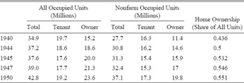
As these comparisons suggest, a key characteristic of increasing home ownership over the early 1940s was that a large part of its supply side involved conversion of the same dwellings from renter- to owner-occupancy. The BLS recorded 2.3 million nonfarm housing starts in the years from 1940 to 1945, most of them in 1940 and 1941. Yet the number of owner-occupied units increased by 4.8 million from April 1940 to November 1945, and the number of nonfarm owner-occupied units increased by 4.5 million, as documented in Table 2. At the same time, the number of renter-occupied units showed an absolute decline of two million units, from 19.7 to 17.6 million; the number of nonfarm renter-occupied units fell by about 0.9 million. Notably, Census data indicate that the 1940s were the only decade of the twentieth century over which the number of renter-occupied units declined, and this decline appears to have occurred only between 1940 and 1945. Supporting the interpretation that these changes reflected conversion of renter-occupied units to owner-occupancy rather than abandonment of deteriorating rental housing, the Census Bureau used cross-tabulations of tenure and year built in the 1950 Census of Housing to estimate that at least 3 million units that were owner-occupied in 1950 had been renter-occupied in 1940 (U.S. Bureau of the Census 1953). The fact that much of the rise in home ownership involved conversions of the same units is consistent with—although certainly not proof of—the hypothesis that rent control induced landlords to sell their properties for owner-occupancy rather than continuing to rent them out.
Table 2 CHANGES IN TENURE, 1940–1950
In part, the size of the increase in home ownership from 1940 to 1945 was associated with the particularly low level of home ownership in 1940 that followed the foreclosures of the Great Depression. Richard Ratcliff (Reference Ratcliff1944) estimated that there were about 600,000 to 700,000 dwelling units that had been owner-occupied in 1930 but were renter-occupied in 1940 due to foreclosure. A substantial share of these were likely in the hands of financial institutions that may have been unwilling landlords, and hence eager to sell them once prices recovered (Fishback, Rose, and Snowden Reference Fishback and Cullen2013; Rose Reference Rose, Fishback, Snowden and White2014). Yet a “rebound” associated with declines in home ownership over the 1930s does not suffice on its own as an explanation for the rapid increase over the early 1940s, at least from the perspective of understanding the supply of dwellings for owner-occupancy. Illustrating this point, Figure 3 plots the city-level change in home ownership over the first half of the 1940s against the city's change in home ownership between 1930 and 1940, for the sample used in the analysis. Surveys were carried out at different times between 1944 and 1946, so the figure plots the residuals from regressions of the city-level changes on survey year fixed effects and within-survey-year time trends. There is a slight (and statistically insignificant) negative relationship between the two, but the change in home ownership over the 1930s does little to explain where home ownership increased over the early 1940s: the partial correlation in the sample, after conditioning on survey timing, is –0.067. Similarly, the city-level 1920–1930 change in home ownership is, if anything, negatively correlated with the change over the early 1940s, with a partial correlation of –0.227. Hence, a “return to trend” is also unlikely to serve as an explanation on its own.

Figure 3 CHANGE IN HOME OWNERSHIP IN THE 1930S AND THE EARLY 1940S
Although the focus on rent control in this analysis puts most of the emphasis on the supply side of the market, it may be helpful to note how these home purchases might have been financed. With incomes rising during the war and little to spend them on, rising personal savings would have helped finance home purchase over the early 1940s. Mortgage lending for home purchase was also active during the war, as aggregate data on home mortgages from the annual reports of the Federal Home Loan Bank Administration from 1941 through 1945 suggest (Federal Home Loan Bank Administration, various years). While overall lending by savings and loans (S&L's), banks, and trust companies decreased in fiscal years 1942 and 1943, individual mortgagees were a substantial share of lending over this period (in fiscal year 1941, they represented 24 percent of the number of mortgage loans and 16 percent of their dollar volume) and mortgage lending by individuals increased with each fiscal year from 1941 through 1945, except for a slight decline in fiscal year 1943. Moreover, the dollar volume of loans given by S&L's for home purchase increased in absolute terms in each fiscal year from 1941 through 1945, despite a decrease in the total volume of S&L lending driven by declines in loans for construction, refinancing, and reconditioning.
THE EFFECT OF RENT CONTROL ON WARTIME HOUSING MARKETS
The results are based on a sample of 51 cities in which the NICB had begun monthly rental surveys by March 1940, for construction of the rent component of its cost-of-living index.Footnote 7 The NICB's choice of sample cities based on characteristics determined prior to 1940 alleviates concerns that the sample would be skewed towards cities experiencing unusual housing conditions during the war. Most of the cities in the NICB sample were relatively large, with all but three having a 1940 population of 100,000 or more. I obtained the values of the NICB rental indices for these cities from National Industrial Conference Board (1941) and from various issues of the Conference Board Economic Record and Management Record. In 1943 the NICB published revisions to its indices for many of the sample cities; in these cases, I use the revised values. Throughout the article, the index is scaled to measure changes in rents relative to their March 1940 level.
City-level data on housing tenure in the mid-1940s come from a set of newly digitized housing surveys carried out by the Census Bureau and the BLS between 1944 and early 1947 (Humes and Schiro Reference Humes and Schiro1946; U.S. Bureau of the Census 1947a, 1948). Surveys were carried out in most large cities, as well as smaller cities that were thought to be experiencing serious housing shortages (Humes and Schiro Reference Humes and Schiro1946). Cities were surveyed at different times; most of the cities in my sample were surveyed in 1945 or 1946, and a few in 1944. The measure of home ownership used is the estimated share of occupied, privately-financed dwelling units that were owner-occupied as of the survey date.Footnote 8 The dependent variable used is the difference between this mid-1940s measure of home ownership and the level of home ownership for the same geographic area in 1940, based on information from the 1940 Census.Footnote 9
For the main results and the robustness checks, I link information on rents and changes in tenure to various characteristics of cities before and during the 1940s. The additional data includes information on the characteristics of war housing built, reported in the September 1945 Consolidated Directory of the Disposition of War Housing (National Housing Agency 1945a) and the growth in county bank deposits from 1941–1944, from the Distribution of Bank Deposits by Counties (U.S. Department of the Treasury 1943, 1945). An additional variable of particular interest, which I have for 35 of the 51 NICB cities, is a measure of the degree of house price appreciation between April 1940 and September 1945. This measure comes from unpublished results of a study carried out by the National Housing Agency (NHA) in the late 1940s (National Housing Agency 1947), which I obtained from the National Archives. This study is the source of the monthly house price series covering Washington, DC from 1918 to 1947 that was reproduced in Ernest Fisher (Reference Fisher1951) and used in the 5-city median house price index of Robert Shiller (Reference Shiller2005). In addition to the monthly series for Washington, DC, the NHA calculated median asking prices for single-family houses that were not newly built and had no commercial features in approximately 80 cities in April 1940, September 1945, and several months in late 1946. Most of the other data come from Michael R. Haines (Reference Haines2010); when possible I use variables reported at the city level, but when necessary I use variables reported for the corresponding county or counties.
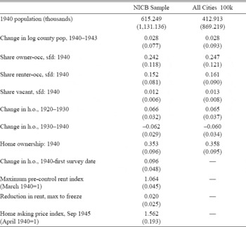
Table 3 reports summary statistics on the 51 cities in the NICB sample. To assess the comparability of the NICB sample with other large cities, I also show statistics for the set of all 92 cities that had a 1940 population of at least 100,000. The cities of the NICB sample tended to have greater population in 1940 than those in the larger set of cities and had slightly less rented single-family housing, but they were quite similar in other respects, suggesting that it is reasonable to expect that the effects found in the NICB sample generalize to a broader class of cities. This table also offers a first look at changes in housing markets in the sample cities over the first half of the 1940s. On average, home ownership rates increased by 9.6 percentage points between the 1940 Census and the city's first survey date. This increase followed an average 6.2 percentage point decline over the 1930s and an average 6.6 percentage point increase over the 1920s. Prior to control, the average city had seen a 6.4 percent rise in rents, and with the imposition of control the average reduction in rents was about 2 percent. Average appreciation in home asking prices suggests that the initial reduction in rents understates the true degree of rent control severity, however: in the 35 cities for which a measure is available, the median asking price in September 1945 was, on average, 56 percent higher in nominal terms than it was in April 1940.
Table 3 MEANS AND STANDARD DEVIATIONS BY SAMPLE
Notes:
The NICB sample comprises the 51 cities tracked by the NICB prior to March 1940 for which data from the Census / BLS tenure surveys are available. Data on home asking prices are available for only 35 of the NICB cities. There were 92 cities of population greater than 100,000 in 1940. “Share owner-occ, sfd” is the share of all dwelling units that were single-family detached and owner-occupied in 1940. “Share renter-occ, sfd” and “share vacant, sfd” are defined similarly (the residual category is housing that was not single family detached). Rent and price indices are nominal. “Reduction in rent” is the difference between the maximum pre-control rent index and the level on the base date, as a share of the maximum pre-control index.
Sources:
See the text.
Since essentially all U.S. cities were placed under rent control during World War II, estimating the effects of rent control on changes in tenure by comparing controlled to uncontrolled areas is not a feasible empirical approach in this setting. Instead I use variation across cities in the initial severity of rent control: the degree to which rent control forced down rents at the time it was imposed. The test takes advantage of the fact that even across cities in which rents rose to similar degrees prior to control—and hence, are likely to have had similar housing demand shocks early in the 1940s—the combination of the OPA's choice of base date and the precise timing of prior rent increases meant that rent control reduced rents by different amounts in different cities. To recapitulate, the idea is illustrated in Figure 1. For each city, the left vertical line marks the base date, and the right vertical line marks the date on which rent control was imposed. The obvious difficulty in comparing Baltimore to Boston is that while rent control had much less initial impact on rents in Boston, this was because Boston had only minimal increases in rents prior to control, and therefore had either a much smaller demand shock or a much more elastic supply of housing than Baltimore. In contrast, the rent indices for Baltimore and Buffalo show similarly large increases in rents from March 1940 to mid-1942. Yet in Baltimore, the choice of base date brought down rents substantially, whereas the choice of base date in Buffalo meant that rent control had much less initial impact on rents.Footnote 10 The spirit of the test is to draw comparisons like that between Baltimore and Buffalo, in order to avoid comparisons in which variation in the severity of control was due, for example, to differences in housing demand. In practice, the main specifications implement this idea by controlling for the maximum degree of rent appreciation prior to control.
The specific measure of severity is the percent decline in rents that would be implied by a reduction in rent from its maximum pre-control level to its level on the base date. That is, it is the difference between the pre-control maximum value of the NICB rent index and its value in the base date month, normalized by the pre-control maximum value.Footnote 11 Using only rental market data as of the date of imposition of control has the advantage that the measure is less influenced by endogenous decisions that potential sellers, tenants, or buyers make in response to rent control. But since the initial reduction in rents will not fully reflect the incentives faced by market participants over the course of the war, the main estimates should be interpreted as reduced-form estimates of the effect of rent control.
The basic regression specification for city i, with first housing survey in year t, is
where Δt(i),40 (home ownership rate) i is the percentage point change in home ownership between April 1940 and the first survey date for city i, carried out in month t (which is hence a function of i). Since the dependent variable is specified as a difference, this specification implicitly controls for time-invariant city characteristics: the right-hand-side controls in the vector Xi allow for differential trends according to city characteristics. I first show the relationship between severity and home ownership conditional only on survey time effects, which account for the fact that cities were surveyed at different times. Except where specified otherwise, the function controlling for common time effects for a given survey month, α(t(i)), is allowed to be piecewise linear, with discontinuities between survey years: I include linear trends by survey month within each survey year, allowed to differ across years, as well as a set of fixed effects for survey year, which allow level shifts by survey year. After showing the raw relationship, I estimate specifications that include various covariates in Xi . As previously noted, among the key controls is the maximum pre-control rent appreciation in city i, which is measured relative to March 1940. The importance of this control is evident in Appendix Figure 1, which illustrates the strong, positive relationship between the measure of severity and pre-control rent appreciation. Other controls included in the baseline specifications are the city's change in home ownership from 1930 to 1940 as well as its change from 1920 to 1930, and three separate controls for the share of housing units in 1940 that were single-family and owned, rented, and vacant. These variables help to capture the possibility that some cities had greater potential for increases in home ownership than others; put differently, they condition on factors in the pre-treatment period likely to be correlated with the elasticity of supply of housing for owner-occupancy.
The relatively small size of the NICB sample makes the downward bias in the usual Eicker-Huber-White robust standard errors a concern. Accordingly, I follow Guido Imbens and Michal Kolesar (Reference Imbens and Kolesar2016) and report HC2 standard errors, along with p-values that correspond to a t-distribution with the degrees of freedom adjustment proposed by Robert Bell and Daniel McCaffrey (Reference Bell and McCaffrey2002).
Table 4 confirms that cities with greater severity had larger increases in home ownership.Footnote 12 Column (1) shows the simple relationship between the size of the rent reduction and the change in home ownership, corrected for survey timing (Appendix Figure 2 shows this relationship graphically). The coefficient suggests that an increase in severity of 2.5 percentage points—roughly a standard deviation in the NICB sample—was associated with roughly a 1.1 percentage point greater increase in home ownership during the early 1940s, with a p-value of 0.023.
Table 4 PERCENTAGE POINT CHANGE IN HOME OWNERSHIP, 4/40 TO SURVEY DATE, AND RENT CONTROL “SEVERITY”

Notes:
HC2 standard errors are in parentheses. Reported p-values correspond to a t-distribution with degrees of freedom determined by the Bell and McCaffrey (Reference Bell and McCaffrey2002) adjustment. “Max pre-control rent” indicates that the specification controls for the degree of rent appreciation from March 1940 to the pre-control maximum. Year fixed effects / trends are fixed effects for survey year and separate linear trends in survey month for each survey year. Baseline controls are the 1920–1930 change in home ownership; the 1930–1940 change in home ownership; and the 1940 share of dwellings that were single-family and owned, rented, and vacant (each entered separately). Additional controls are the log median house value in 1940, the log average rent in 1940, the nonwhite population share in 1940, and Census region fixed effects (allowing regional trends). For covariate coefficient estimates, see Appendix Table 1.
Sources:
See the text.
The main test of the rent control hypothesis is the specification in column (2), which adds a control for the maximum pre-control rent appreciation, as well as the baseline set of controls described earlier. The relationship between severity and increased home ownership does not appear to be driven by the degree of pre-control rent appreciation, and hence does not merely reflect, for example, differential housing demand growth. The coefficient on severity in fact increases slightly in this specification, and remains significant at a reasonable level, with a p-value of 0.082. The point estimate suggests that severity greater by 2.5 percentage points led to roughly a 1.2 percentage point greater increase in home ownership over the early 1940s (Appendix Figure 3 illustrates this relationship). Finally, in column (3) I add additional controls to allow differential trends by Census region and by other 1940 city characteristics—house values and rents in 1940 and the nonwhite share of the population. Doing so has little effect on the size or statistical significance of the coefficient on rent control severity.
The primary focus of this article is the effect of rent control on home ownership, but a closely related question is the impact that it had on prices for owner-occupancy. To the extent that excess demand from unsatisfied consumers in the rental market spills over into the owner-occupied market, there will be upward pressure on house prices. Consistent with this mechanism is the 56 percent average rise in the home asking price index from April 1940 to September 1945. In general, however, it is ambiguous whether rent control should increase or decrease prices in the uncontrolled market for owner-occupied dwellings, as a long-running literature has discussed (Fallis and Smith Reference Fallis and Smith1984). Several other factors may play a role as well. For example, Autor, Palmer, and Pathak (Reference Autor, Palmer and Pathak2014) note that control of rental units may affect house prices through externalities related to maintenance and residential sorting; they find that the removal of rent control in Cambridge in the mid-1990s raised values of uncontrolled housing.
To assess the effect of rent control on house prices in this setting, I estimate specifications similar to equation (1) with home asking price appreciation from April 1940 to September 1945 as the dependent variable. The measure of house price appreciation is available for 35 of the sample cities. Unfortunately, the NHA's criteria for choosing a sample of cities to survey for house prices were not clearly specified, but it can be said that these 35 cities had similar average growth in home ownership to the full NICB sample of 51 cities (9.6 percentage points for the full set of 51 and 9.4 percentage points for the subsample with price appreciation data), and also that rent control severity is not a statistically significant predictor of the presence of price data either in an unconditional specification or conditional on the main set of controls used above.Footnote 13
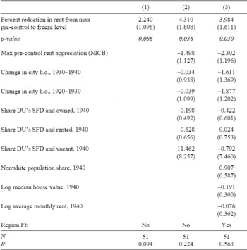
The results in Table 5 suggest that cities with greater initial rent control severity saw greater house price appreciation from 1940 to 1945; Appendix Figure 4 illustrates this relationship.Footnote 14 In particular, the specification in column (3), which contains the full set of controls, gives a coefficient of 3.984 (and a p-value of 0.030), suggesting that an initial level of severity greater by 2.5 percentage points (a standard deviation in the full sample) was associated with appreciation in house prices that was greater by 10 percentage points. In the context of World-War II era housing markets, it appears that rent control tended to increase prices for owner-occupancy.

Figure 4 COEFFICIENTS AND 90 PERCENT, 95 PERCENT CONFIDENCE INTERVALS USING “PLACEBO” BASE DATES
Table 5 HOME ASKING PRICE APPRECIATION, 4/40–9/45, AND RENT CONTROL “SEVERITY”

Notes:
HC2 standard errors are in parentheses. Reported p-values correspond to a t-distribution with degrees of freedom determined by the Bell and McCaffrey (Reference Bell and McCaffrey2002) adjustment. “Max pre-control rent” indicates that the specification controls for the degree of rent appreciation from March 1940 to the pre-control maximum. Baseline controls are the 1920–1930 change in home ownership; the 1930–1940 change in home ownership; and the 1940 share of dwellings that were single-family and owned, rented, and vacant (each entered separately). Additional controls are the log median house value in 1940, the log average rent in 1940, the nonwhite population share in 1940, and Census region fixed effects (allowing regional trends).
Sources:
See the text.
ASSESSING ROBUSTNESS TO ALTERNATIVE EXPLANATIONS
The identifying assumption in the main specifications is that conditional on the maximum pre-control rent appreciation, the reduction in rents induced by rent control was unrelated to underlying city trends that were also associated with differential trends in home ownership. In this section, I offer three complementary pieces of evidence supporting a causal interpretation of the estimates.
Exploiting the “Default” Base Date
The variation in the initial severity of rent control in the main specifications comes from the combination of the OPA's choice of base date and the timing of increases in rent. My first approach to assessing the identification assumption is to use the OPA's “default” base date to isolate variation in rent control severity that does not rely on city-specific choices of the OPA, but instead relies only on variation in the timing of rent increases across cities. I then assess whether the variation in timing of rent increases is likely to be related to unobserved factors that also led to greater growth in home ownership.
The OPA devoted much attention to setting city-specific base dates in the initial wave of rent control imposition in the summer of 1942, and a number of different base dates were used. By October 1942, however, nearly all newly controlled counties were assigned the default base date of 1 March 1942: 92 of 97 counties controlled in October, 197 of 198 counties controlled in November, and 111 of 112 counties controlled in December. Twenty cities in my sample were put under control over these three months, and all shared the common base date. I re-estimate a variant on my main specification on the sample of cities controlled between October and December 1942, making it slightly more parsimonious given the smaller size of the sample.
By controlling for maximum pre-control rent appreciation and testing for differences in increases in home ownership in cities that had sharper initial rent reductions when rolled back to March 1942, this specification exploits variation in the precise timing of rent increases. The spirit of this test is to draw comparisons between two cities in which rents rose by similar amounts prior to control at the end of 1942, but in which rents had risen by different amounts as of March 1942. A city where most of the rent increase happened by March 1942 would have lower severity, and one where most of the increase happened after March 1942 would have greater severity. The identification assumption is that given that cities eventually had similar rent increases before control, the degree of rent appreciation by March 1942 was unrelated to unobserved factors that drove differential trends in home ownership.
The point estimates in Table 6 for this 20-city sample suggest that the possible correlation between the OPA's choice of base dates and unobserved factors increasing home ownership does not induce upward bias in the main estimates. The coefficient in column (3), which controls for the maximum pre-control rent appreciation and survey timing in the same way as the main specifications, suggests that a severity greater by 1 percentage point was associated with a 1.6-percentage point greater increase in home ownership over the 1940s. The point estimate is somewhat larger than those in the main specifications. Taking this result at face value, it may be that the OPA's choice of city-specific base dates induces a downward bias in the main results. For example, suppose that defense production stimulates demand for rental housing more than for owner-occupied housing because it is expected to be a temporary labor demand shock. If the OPA chose base dates to reduce rents more in cities where rent increases were associated with defense activities, as the institutional background suggests, then greater rent control severity should have been related to greater demand shocks for rental, not owner-occupied, housing. Given the wide confidence intervals in column (3), however, the difference in point estimates may not be very meaningful.
Table 6 RENT CONTROL SEVERITY AND CHANGE IN HOME OWNERSHIP FOR CITIES CONTROLLED 10/42–12/42

Notes:
HC2 standard errors are in parentheses. Reported p-values correspond to a t-distribution with degrees of freedom determined by the Bell and McCaffrey (Reference Bell and McCaffrey2002) adjustment. Baseline controls are the 1920–1930 change in home ownership; the 1930–1940 change in home ownership; and the 1940 share of dwellings that were single-family and owned, rented, and vacant (each entered separately). Within-year trends only estimated for 1945 and 1946 (all 1944 observations were surveyed in September).
Sources:
See the text.
The identifying assumption for this robustness check is that conditional on the eventual degree of pre-control rent appreciation, the precise timing of the appreciation was not correlated with unobserved factors that themselves led to greater increases in home ownership between 1940 and the mid-1940s. To evaluate the plausibility of this assumption, I re-estimate the specification in column (3) of Table 6 using months from March 1941 to February 1942 as placebo base dates. If the relationship between rent control severity and home ownership is due to unobserved factors associated with early rent increases, then it is likely that it should not matter whether “early” means prior to March 1942, or instead means prior to September 1941 (to choose one example). That is, calculating rent control severity as the implied reduction to base dates other than March 1942 should produce similar results. Note that since rents are serially correlated, as the placebo dates approach the true base date we should expect them to deliver larger and more significant effects—in the extreme, a “placebo” date one day prior to the actual base date would deliver estimates essentially identical to those from using the actual base date, not really being a “placebo” at all. In the absence of a clear criterion for determining which dates are too close to the true base date to be considered “placebo” base dates, I include results using placebo dates close to the true base date, but the results should be interpreted with this caveat in mind.
I show the coefficients and confidence intervals for each placebo date as well as the true one in Figure 4. The results support the identifying assumption. Conditional on the eventual degree of rent appreciation, “later” rent appreciation does not appear to be correlated with greater increases in home ownership except when it coincides with greater rent control severity. Using any of the months from March through December 1941 as a placebo base date delivers estimates that are not statistically significantly different from zero, and for which the point estimates themselves are relatively close to zero. Only when the placebo base date approaches the true base date do the estimates begin to come close to the estimate in Table 6. As noted above, due to serial correlation in rents we would expect to begin seeing larger and more significant effects as the placebo dates approach the true one, which indeed is what is observed in the data.
Introducing Controls for Alternative Explanations
There are several other candidate explanations for unusually sharp increases in home ownership rates during the early 1940s, and one might be concerned that these are correlated with the variation in rent control severity even conditional on the degree of rent appreciation prior to control. One possibility is that rising incomes and savings encouraged a shift towards ownership as a form of housing tenure. Another is that the wartime rise in marginal income tax rates made the non-neutralities in the tax code between owner- and renter-occupied housing more relevant than they had been before, driving a shift towards owner-occupancy (Rosen and Rosen Reference Rosen and Rosen1980). The abnormally low level of home ownership in 1940, after the foreclosures of the 1930s, may have led to an unusually fast increase as the “overhang” of properties was sold off. Finally, the war economy may have raised expectations of future growth and encouraged home purchase. As a second approach to supporting a causal interpretation of the main estimates, I assess whether or not these alternative explanations are likely to explain the main result by introducing additional controls that should provide measures of geographic variation in these alternatives. Many of these variables could plausibly be affected by rent control itself, so the coefficient estimates in these specifications should be interpreted with caution; the spirit of this exercise is to see whether inclusion of these variables leads to a substantial reduction in the severity coefficient.
The results shown previously, in fact, already address two of these alternative hypotheses. Column (1) of Table 7 reproduces the final column from Table 4. This specification already controls for the city's 1930–1940 and 1920–1930 changes in home ownership, making it unlikely that the rent control result is driven by depressed levels of home ownership in 1940. It also addresses the possibility that rising marginal tax rates increased home ownership during the war. Work studying geographic variation in housing tax benefits over the 1980s and 1990s (Gyourko and Sinai Reference Gyourko and Sinai2003, Reference Gyourko and Sinai2004) uses more extensive data than are available for my sample, but as a rough approximation, differential changes in the tax benefit to owner-occupied housing as income tax rates rose during the 1940s should be correlated with city housing values in 1940. Column (1) includes a control for the median owner-occupied housing value in 1940, and as seen in Table 4, inclusion of this control did little to change the size of the severity coefficient. Hence, it is unlikely that spatial variation in the tax benefit to owner-occupied housing explains the rent control result.
Table 7 ROBUSTNESS TO ALTERNATIVE EXPLANATIONS

Notes:
HC2 standard errors are in parentheses. Reported p-values correspond to a t-distribution with degrees of freedom determined by the Bell and McCaffrey (Reference Bell and McCaffrey2002) adjustment. All specifications control for maximum pre-control rent; the 1920–1930 change in home ownership; the 1930–1940 change in home ownership; the 1940 share of dwellings that were single-family and owned, rented, and vacant (each entered separately); log median house value in 1940; log average rent in 1940; nonwhite population share in 1940; region fixed effects; survey year fixed effects; and within-survey year time trends. Per capita E-bond sales and war spending per capita are measured in thousands of dollars.
Sources:
See the text.
I address a range of other concerns in columns (2) through (6), adding controls that are likely to be correlated with income, savings, and expectations of future city growth (in Appendix Table 3 I introduce each individually). There is no data directly measuring city- or county-level personal incomes over this period, so I use two alternative measures: the change in log retail sales per capita from 1939–1948, following Fishback and Cullen (Reference Fishback and Cullen2013), and the change in the log total dollar value of manufacturing wages from 1939 to 1947. As a first proxy for savings, I use the 1941–1944 change in log bank deposits. I also include a control for county E-bond sales per capita. Both of these types of savings could of course substitute for saving in the form of housing, but it may be that differential shocks to the ability to save translated into greater saving in all forms. Two final controls in column (2) are the change in log county civilian population from 1940 to 1943 and total county World War II spending from 1940–1945 (normalized by the 1940 population). These variables are meant to serve as additional controls for the size of the housing demand shock across cities. To proxy for expectations of future growth, I control for the share of war housing that was privately financed. The rationale for doing so is that when future demand for housing was uncertain, war housing tended to be publicly financed (National Housing Agency 1945b). An alternative, which focuses on changes in expectations prior to restrictions on construction, is to use data on city-level building permits before the end of 1941 as a measure of anticipated housing demand at the beginning of the 1940s. I use the number of new housing units authorized in 1940 and 1941, from the U.S. Bureau of the Census (1966), normalized by the number of dwelling units in 1940.
The results suggest that the rent control result is not driven by correlated trends in incomes, savings, or housing demand. Including controls for income, savings, county war spending, and population change reduces the coefficient on severity only modestly, from 0.465 to 0.419. Data on financing of war housing are unavailable for two cities in my sample, so in column (3) I re-estimate the baseline specification omitting these two, and add a control for financing of war housing in column (4). The coefficient of 0.413 is again close to the 0.465 that I estimate in the baseline specification. Data on permits are unavailable for six cities in the sample, so in column (5) I re-estimate the baseline specification omitting these six, and control for permits in 1940 and 1941 in column (6). The results are quite imprecise but the point estimate on severity is not dramatically changed by the inclusion of the final control. Altogether, the evidence in Table 7 suggests that these alternative stories do not explain the relationship between rent control severity and increased home ownership.
Evidence from the Timing of Imposition
Use of an entirely different source of variation—the timing of rent control imposition across cities—provides a final approach to supporting the interpretation of the main estimates. There is no data on housing tenure at a sufficiently high temporal frequency to use this test to examine shifts into home ownership directly, but changes in the number of newspaper advertisements offering houses for sale is likely to provide a rough measure of the degree to which property owners chose to attempt to sell in response to the imposition of rent control.Footnote 15 For one newspaper from each of nine cities, I have collected data on the number of ads offering houses for sale on the first Sunday of each March, June, September, and December from 1939 to 1946. Details on the sample and the data construction are given in the data appendix. Although the sample is small, there is a reasonable degree of variation in timing of rent control across the nine cities: one was controlled in 1941q4, two in 1942q2, three in 1942q3, two in 1942q4, and one in 1943q4.
The basic specification is

for city c observed in quarter t. This specification controls flexibly for fixed city characteristics and time shocks common across cities. It also allows an assessment of the identifying assumption by testing whether cities appeared to be on different trends in sales prior to the imposition of control. I estimate a separate coefficient for each relative quarter from seven quarters prior to seven quarters following control, plus a common coefficient for all quarters eight or more before and one for eight or more after control. The omitted category is the quarter immediately preceding the quarter in which rent control was imposed. In the preferred specifications, I augment equation (2) by controlling for city-specific linear time trends and city-specific season (quarter of year) fixed effects. The motivation for including the latter is pronounced seasonality in advertisements that appears to have been specific to a few cities in the sample. I estimate standard errors clustered by city; following Imbens and Kolesar (Reference Imbens and Kolesar2016), I use the Bell and McCaffrey (Reference Bell and McCaffrey2002) adjustment for both standard errors and hypothesis testing to account for the small number of clusters (nine).
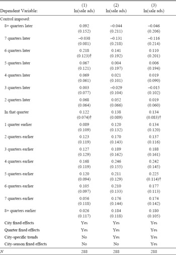
Figure 5 plots the estimates of γt for the log number of sale advertisements, from a specification that augments equation (2) with city-specific trends and city-season fixed effects. These coefficients and those from alternative specifications are also shown in Appendix Table 4. There is little indication of a differential trend in sale ads pre-dating the imposition of rent control. The coefficients for the first period of control and afterwards indicate a differential uptick in the number of sale ads immediately after the imposition of rent control, with a number of sale advertisements about 0.2 log points higher about a year after the imposition of control. The results are quite imprecise, as would be expected with only nine clusters, so caution is clearly merited in interpreting the estimates. But taken together, they provide suggestive evidence supporting the interpretation of the main estimates, that rent control induced property owners to put their properties on the market for owner-occupancy.

Figure 5 LN(NUMBER OF SALE ADS) RELATIVE TO QUARTER PRIOR TO CONTROL
HOW MUCH OF THE INCREASE IN HOME OWNERSHIP CAN RENT CONTROL EXPLAIN?
The results so far indicate that wartime rent control increased urban home ownership; a natural question is what share of the large wartime increase in home ownership rent control can explain. The main regression results can be used to answer the question of how much home ownership would have increased in the sample cities if the initial reduction in rents had been zero in all cities, which would correspond to setting the frozen level of rents at their peak pre-control levels rather than reducing them. Even in cities where rents were not initially reduced under rent control, however, keeping rents at their pre-control levels would still have been a reduction in rents relative to what they would have been in the absence of rent control, as housing demand grew over the course of the war. Hence, house price appreciation over the course of the war would have increased the relative return to selling rather than renting out housing, since rents were still frozen at their nominal pre-control values. To give an idea of the quantitative magnitudes, in 21 of the 35 cities for which price appreciation data are available, the initial reduction in rents implied by a return to the base date was less than half a percent. The rent increases in these cities prior to control ranged from 0.3 percent to 9.6 percent, with an average of 4 percent. By September 1945, nominal asking prices in these 21 cities had risen 56 percent on average, and 15 percent at a minimum. The magnitude of house price appreciation suggests significant growth in the relative return to selling between the imposition of control and the observation of home ownership rates in the mid-1940s. A back-of-the-envelope calculation simulating home ownership rates around the end of the war in the counterfactual scenario of zero initial rent reductions in all cities is therefore likely to give a lower bound for the overall contribution of rent control to the increase in home ownership during the early 1940s.Footnote 16
Of the 51 sample cities, there are 50 with estimates of the number of occupied dwellings on the tenure survey date (necessary to calculate a home ownership rate for the cities as a group). In these cities as a group, weighting by each city's share of all occupied dwellings, the increase in home ownership was 7.76 percentage points. Using the coefficient on initial severity of 0.465 estimated in column (3) of Table 4, the predicted increase in home ownership if the initial severity of control had been zero in all cities—that is, if rents had been frozen at their peak pre-control levels in all cities rather than reduced in some cities—is 7.03 percentage points. This calculation suggests that rent control can explain at least 9.4 percent of the increase in home ownership in the sample cities over the early 1940s.
CONCLUSION
World War II coincided with extraordinary changes in urban housing markets, of which one of the most notable was the rapid increase in home ownership. While other periods of rising home ownership over the last century have been associated with construction of new housing, the extremely limited amount of construction during the war meant that a substantial share of the increase in home ownership over the early 1940s came from shifting existing structures from renter- to owner-occupancy. This fact shifts the focus to the incentives facing property owners to sell their properties for owner-occupancy rather than to rent them out.
In a new dataset on city-level changes in tenure, rents, and house prices during the first half of the 1940s, I show that conditional on the degree of pre-control rent appreciation, cities in which rent control was more severe at the time of control—as measured by the degree to which control was meant to lower rents—had greater increases in home ownership. This relationship is stable across specifications that allow for differential trends by a variety of pre-1940 characteristics, and is not explained by differential changes in income, savings, tax benefits to home owners, expectations across cities, or endogenous choice of base dates. The estimates suggest that rent control can explain at least 10 percent of the urban increase in home ownership over the early 1940s.
An open question is what role rent control played in the longer-run increase in home ownership. It is not unreasonable to suppose that it may have had persistent effects: landlords' experience under rent control, for instance, may have discouraged subsequent investment in rental housing. A large increase in home ownership rates as a result of temporary factors may also have affected the political economy of home ownership. For example, home purchases among lower-income groups in the immediate postwar period, when rent control was still in effect in many areas, were cited as one of the reasons behind the introduction of the exclusion of capital gains on the sale of a principal residence in 1951 (U.S. Congress 1951).
More broadly, the attentiveness of home owners to local politics (Fischel Reference Fischel2001) suggests that the rapid creation of a large new group of home owners may have exerted substantial influence on local political decisions well into the postwar period. It would be interesting for future research to explore the effects of the rapid wartime increase in home ownership on local government or on the course of postwar suburbanization.
Appendix DATA CONSTRUCTION
51-City Sample
As described in the text, the sample for the main regressions comprises repeated observations for 51 cities in which the NICB had begun tracking rents by March 1940. By that point the NICB had actually began tracking rents in 56 cities, but two, Minneapolis and St. Paul, had a combined tenure survey, and four had no tenure survey (these were Lansing, Michigan; Lynn, Massachusetts; Oakland, California; and Wausau, Wisconsin—Lynn and Oakland were, in fact, surveyed, but only as part of much larger Boston area and San Francisco Bay area surveys).

Appendix Figure 1 “SEVERITY” OF RENT CONTROL AND RENT APPRECIATION PRIOR TO CONTROL
The tenure surveys provide data at various levels of geographic aggregation, and using them to measure changes relative to 1940 requires some care in identifying comparable geographic areas for the 1940 values. Sometimes survey data is provided for the city boundaries, sometimes for county boundaries, and sometimes for “areas” encompassing multiple cities or a city and surrounding areas. When multiple levels of geographic aggregation are available for a city, I choose survey data according to the following rules of precedence. Having chosen the surveys, I then use the earliest tenure survey available for each city.
-
(1) When surveys following the city boundaries were available, I used those, and excluded any surveys at the area level. This group included 32 of the final 51 cities.
-
(2) If no survey at the city level was available but there was a survey at the county level, I used those (and excluded any survey at the area level for the same city). This group included three cities: Los Angeles (Los Angeles County), Cleveland (Cuyahoga County), and Newark (Essex County).
-
(3) If there was no survey for a single city but there was for a pair of cities (without surrounding areas outside of the cities), I used the pair of cities. This group included two pairs of cities: Minneapolis-St. Paul and Duluth-Superior.
-
(4) If surveys were not available at either the city or county level, I used data at the “area” level (encompassing the primary city and one or more surrounding smaller areas). This group included the remaining 14 cities in the sample.
For 4 of the 14 surveys at the “area” level, the surveys reported 1940 tenure figures for an area that covered the same area as the intercensal survey, and in 5 of the “area”-level surveys the 1940 tenure figures covered between 95 and 100 percent of the intercensal survey area. Of the remaining five surveys at the area level, four have no 1940 data reported with the intercensal surveys and one has data reported for a 1940 area covering only 85 to 95 percent of the intercensal survey area. For these five, I reconstruct 1940 home ownership numbers for a comparable area using the reported area definitions and the minor civil division data from the 1940 Census, referring to the original survey reports to identify the survey areas when necessary.

Appendix Figure 2 CHANGE IN HOME OWNERSHIP AND “SEVERITY” OF RENT CONTROL (NET OF SURVEY TIMING)
A related issue is that for cities that annexed land between 1940 and the first tenure survey and which subsequently had tenure surveys reporting figures for the city, it is not always clear whether the boundaries followed were the original ones or those after annexation. In my sample, there are 8 cities that had annexed more than half a square mile of land between 1940 and the year of the first tenure survey (based on information from various issues of the Municipal Year Book (Ridley and Nolting, various years)) and whose survey reported figures at the city level.
Ultimately, any area inconsistencies in the tenure measures do not appear to be a concern. There are 13 cities in which area comparability may be an issue: those that (a) were surveyed at the area level but with coverage between 95 and 100 percent, or (b) were surveyed at the city level and annexed more than half a square mile of land before the first tenure survey. Omitting these 13 cities from my sample strengthens the results reported in the text.

Appendix Figure 3 CHANGE IN HOMEOWNERSHIP AND “SEVERITY” OF RENT CONTROL (NET OF ALL BASELINE CONTROLS)
Several control variables are measured at the city level, regardless of the geographic extent of the tenure survey. These include the 1920–1930 and 1930–1940 changes in home ownership, and the variables on occupancy and tenure by structure type. For three observations I combine two cities to calculate these control variables (these are Minneapolis-St. Paul, Duluth-Superior, and the Fall River-New Bedford area). The NICB rent indices are also measured at the city level.
To calculate control variables at the county level, I aggregated data from all counties in which a sample city (or pair of cities, for Minneapolis-St. Paul and Duluth-Superior) had population in 1940. The one exception is Youngstown, Ohio, which had 99.9 percent of its 1940 population in Mahoning County.
Newspaper Advertisements
The data on advertisements of housing for sale comes from nine cities for which digital images of classified ads were available consistently throughout the sample period, with headings in the classified ad section that allow a straightforward classification of ads into offered sales (as opposed to, for example, houses either for sale or for rent). The nine newspapers are the Chicago Tribune, the Cleveland Plain Dealer, the Dallas Morning News, the Los Angeles Times, the New Orleans Times-Picayune, the New York Times, the Portland Oregonian, the Seattle Times, and the Washington Post. In each city, I use the count of ads appearing on the first Sunday of each March, June, September, and December. I include housing in the city or suburban areas. For the New York Times, I exclude ads for housing in suburban areas that were put under control before or after the first wave of rent control in New York City (for example, counties in New Jersey, Connecticut, and some nearby counties in New York state were put under control either earlier or later than New York City was).

Appendix Figure 4 HOUSE PRICE APPRECIATION AND “SEVERITY” OF RENT CONTROL (NET OF ALL BASELINE CONTROLS)
I attempt to exclude certain types of advertisements from the count of sale ads. Among the excluded ads are those for the sale of unimproved land; ads for the sale of “income property,” such as apartment buildings or farms; ads for summer homes, beachfront or resort properties; ads for exchange of real estate; ads for home building or financing; and ads offering homes “for rent or sale.” A caveat is that sometimes ads for empty lots are included in the same classification as ads for homes in suburban areas. As a rule, the counts include or exclude entire classifications of ads, rather than trying to distinguish between different types of ads under the same classification. Hence, when ads for empty lots are included under classifications that primarily advertise homes, they are included in the total count. Some ads advertise multiple properties, but since many of these do not specify the exact number available, I use counts of the number of distinct advertisements rather than the number of distinct properties.
Appendix Table 1 CHANGE IN HOME OWNERSHIP, 4/40 TO SURVEY DATE, AND RENT CONTROL “SEVERITY”

Appendix Table 2 HOME ASKING PRICE APPRECIATION, 4/40–9/45, AND RENT CONTROL “SEVERITY”
Appendix Table 3 ROBUSTNESS TO ALTERNATIVE EXPLANATIONS

Appendix Table 4 NEWSPAPER ADS: RESPONSE TO IMPOSITION OF RENT CONTROL