The American Civil War was a bloody and destructive conflict that left many survivors with hard feelings and bitter memories. We explore how the deeply divisive ideology of the post-bellum era influenced migration decisions of Civil War veterans. In The Myth of the Lost Cause and Civil War History, Gary Gallagher and Alan Nolan (2000) explain that sectionalism was so intense that survivors from opposing sides did not even remember the war in the same way. It is clear from the historical record that many Union and Confederate veterans felt a deep antipathy for one another, leading, in some cases, to violence (Wiley Reference Wiley1943; Wiley Reference Wiley1951; Astor Reference Astor2012). The war experience so fundamentally influenced the evolution of both northern and southern culture in the post-bellum period that adherents to one side often felt deeply unwelcome in a place sympathetic to the other side (Blight Reference Blight2001; Marshall Reference Marshall2010; Radford Reference Radford1992; Vinovskis Reference Vinovskis1989). We explore whether these ideological differences were related to the choice to move as well as the destination of those who moved after the war by focusing on survivors from border areas, which sent soldiers to both the Union and Confederate Armies.
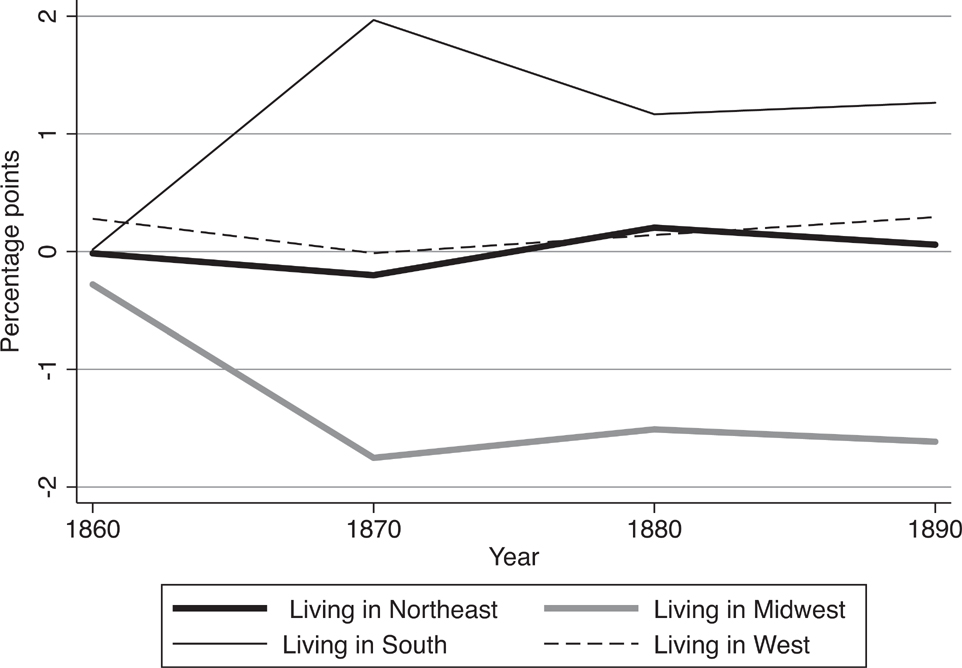
Because most Union supporters were northerners and most Confederate supporters were southerners, it is difficult to separate decisions to migrate that were motivated by ideology from those motivated by economics or information. Some evidence in favor of ideology comes from an examination of aggregate census data, which suggests that the rate of south-to-north migration among whites declined after the Civil War. Specifically, the fraction of southern born whites residing in the South increased by 2 percentage points between 1860 and 1870 and continued to increase through 1890, with a corresponding decline in the fraction of southern born whites residing in the Midwest (see Figure 1). William Collins and Marianne Wanamaker (Reference Collins and Wanamaker2015) also find that few southern whites migrated to the Northeast or Midwest during this period and speculate that this was driven by poor relations between northerners and southerners.

Figure 1 Change in Fraction of Southern Born Whites, Relative to Previous Census Year
To further explore the relationship between ideology and migration in the aftermath of the Civil War, we study individuals from the border state of Kentucky. This context provides a unique opportunity because Kentucky contributed many enlistees to both the Union and Confederate Armies, often from the same communities. Moreover, soldiers from both sides can be identified using Kentucky enlistment records and then followed over time by linking individuals to federal census records. This linking allows us to control for observable differences between Union and Confederate recruits. While focusing on Kentucky does not allow us to generalize about the entire United States, we believe our setting offers the clearest possible evidence that Union and Confederate recruits migrated to avoid one another.
We construct a novel longitudinal database of Union and Confederate recruits from Kentucky by matching military records from the state’s regiments to the 1860 census of population. We then link recruits forward to the 1880 census. We are able to observe each recruit’s socioeconomic status in addition to his county of residence prior to enlistment, which allows us to infer whether recruits were living in places where Union or Confederate status would have been socially rewarded. The longitudinal data also allow us to address concerns that differential migration patterns were the result of differences in skill as opposed to social rewards or penalties from military service. For instance, if Union recruits were systematically less skilled, and the returns to skill were higher in counties sympathetic to the Confederacy, we should expect Union veterans to leave Confederate-leaning counties for economic reasons alone (Borjas Reference Borjas1987). Therefore, the ability to observe ex-ante characteristics of recruits, such as occupational attainment and wealth, is a major advantage of our research design.
We document a series of facts about how ideology, socioeconomic characteristics, and participation in the Civil War interacted to shape the migration behavior of veterans from Kentucky. First, although Confederate enlistees tended to come from wealthier families, Union and Confederate veterans migrated from their home counties at similar rates. However, Union soldiers were more likely to migrate the greater the support for the Confederacy in their home counties. These veterans settled in counties that were more pro-Union on average. Confederate soldiers, for their part, were more likely to choose Confederate-leaning counties in Kentucky, or states in the far West or South, if they moved. More than half of Kentucky enlistees migrated out of their home county between 1860 and 1880, so the scope for sorting was significant.
We also find that the drive to migrate was stronger for veterans themselves compared with their family members: relatives who were not found in our enlistment records were both less likely to migrate and less responsive to the ideology of their home county. If these family members did move, however, they exhibited a similar preference for destination counties whose residents shared the political opinions of their veteran relative. We conclude our analysis by considering whether or not the gains from migration differed by military side. Although we do not find evidence of a differential return to migration for Union and Confederate veterans— many of whom were farmers—in terms of occupational income, we do find that Union recruits moved to places with better agricultural land.
Our findings relate to the literature in economic history on the post-Civil War outcomes of Union Army veterans. Dora Costa (Reference Costa1995, Reference Costa1997) uses Union Army veterans to study the impact of pension income on retirement and living arrangements, Shari Eli (Reference Eli2015) studies income effects on the health of Union Army veterans, and Laura Salisbury (2017) investigates the impact of Union Army widows’ pensions on remarriage. Hoyt Bleakley, Louis Cain, and Joseph Ferrie (2014) study labor market discrimination among Union Army veterans. Costa and Matthew Kahn (Reference Costa and Kahn2008) explicitly measure the impact of the war on veterans by examining how unit cohesion affects later-life outcomes and find that deserters were more likely to leave their home towns after the war. In more recent work, Costa, Kahn, Chris Roudiez, et al. (Reference Costa, Kahn and Roudiez2016) find that Union Army veterans co-located with men from their former companies. Given this literature, a distinguishing feature of our article is that we are able to study the migration behavior of both Union and Confederate Army veterans. Both groups preferred to live in like-minded communities.
Our work also sheds light on post-bellum migration in the United States more generally. In the decades immediately after the American Civil War, average income in the South was persistently low relative to the North (Wright Reference Wright1986; Rosenbloom Reference Rosenbloom1990). However, despite this disparity, relatively few southern whites migrated out of the former Confederacy into Union states (Rosenbloom Reference Rosenbloom1990).Footnote 1 While north-south migration in the United States has always been less common than east-west migration (Steckel Reference Steckel1983), the magnitude of the wage differential in the post-bellum period makes this particular instance of low migration notable. Economic historians have hypothesized that the lack of migration was the result of the irreversibility of investments that southerners had made in cotton agriculture (Wright Reference Wright1986) and by a lack of information in the South about labor market opportunities in the North (Rosenbloom Reference Rosenbloom1990). Institutional barriers to out-migration, such as anti-enticement laws, were predominantly aimed at southern blacks (Naidu Reference Naidu2010) and thus unlikely to explain why white southerners were so unwilling to move after the war. Our results provide empirical support for the notion that ideology could also explain the relative lack of migration from the South to the North.
Historical Background
Kentucky During the War
The Civil War began on 12 April 1861, when Confederate ships attacked the Union Army at Fort Sumter in South Carolina, and the war ended on 9 April 1865, when Robert E. Lee surrendered at Appomattox Courthouse in Virginia. Approximately 2.2 million men served on the side of the Union and 1.1 million men served for the Confederacy. Kentucky was one of four “border states,” or slave-owning states that did not secede from the Union; Missouri, Maryland, and Delaware were the others. In Kentucky, as in other border states, pro-Confederate and pro-Union supporters lived alongside each other (both Union President Abraham Lincoln and Confederate President Jefferson Davis were born in Kentucky). Kentucky’s economy relied on markets in the Union and the Confederacy: tobacco, whiskey, and flour produced in Kentucky were exported to the South and Europe via the Ohio and Mississippi rivers and to the North by rail. Kentuckians were split on the issue of slavery. Although most did not own slaves, some Kentuckians were heavily involved in the profitable export of slaves to the Deep South.
In general, ante-bellum Kentucky was solidly pro-slavery but decidedly more moderate on secession than most states in the Deep South. This view was common in border states, where all governors elected during the late 1850s were pro-slavery Democrats (Phillips Reference Phillips2013, p. 5). At the same time, as Aaron Astor (Reference Abramitzky, Boustan and Eriksson2012, p. 9) argues, Kentuckians and other border residents “rarely viewed the national debates over slavery as irreconcilable” due to the state’s social ties with the Midwest and the frequency with which free wage labor and hired slave labor interacted in factories and farms.Footnote 2 This relative moderation is clear from Kentucky’s returns in the 1860 presidential election, in which the westward expansion of slavery was a major campaign issue. Northern states voted overwhelmingly in favor of Abraham Lincoln’s Republicans, who explicitly favored banning slavery in all U.S. territories, and Southern states voted overwhelmingly in favor of John C. Breckenridge’s Southern Democrats, who explicitly favored the protection of slavery in the territories. Meanwhile, Kentucky voted in favor of John Bell, who headed the Constitutional Union Party and did not take a strong stance on the westward expansion of slavery. This party consisted largely of moderate ex-Whigs who found the Republican Party too radical; the party’s platform avoided the question of slavery in the territories altogether. Bell carried 60 of Kentucky’s 110 counties, and Breckenridge placed second, carrying 43 counties (Harrison Reference Harrison1975, p. 4).
While Kentuckians did consider the possibility of secession, most families were “Conservative Unionists” (Astor Reference Astor2012; Phillips Reference Phillips2013). It was also not the case that all slave-owners wished to secede while all non-slave-owners wished to remain in the Union: many Kentucky slaveholders felt that their interests were better served within the Union than outside it. This inclination was likely related to Kentucky’s shared northern border with free states, and concern about relinquishing the protections they enjoyed under the Fugitive Slave Act. As prominent attorney Joseph Holt argued, if Kentucky were to secede, it would “virtually have Canada brought to her door, denying the state’s slaveholders legal protections to prevent enslaved people from fleeing northward to freedom” (Phillips Reference Phillips2013, p. 12).
Kentucky initially tried to remain neutral, but this stance proved untenable when the Confederate Army invaded in the fall of 1861 and federal troops subsequently occupied the state. While the majority of Kentuckians initially favored remaining in the Union, public opinion changed over the course of the war (Astor Reference Astor2012; Marshall Reference Marshall2010). Many Conservative Unionists objected to Lincoln’s troop call-up and the behavior of federal troops in their state. Even though the Emancipation Proclamation was not applicable in the state, many Kentuckians were ideologically opposed to the emancipation of slaves and their enlistment in the Union Army. At the same time, many felt alienated by Confederate raids during 1862 and 1863 (Harrison Reference Harrison1975). While few Kentuckians formally switched allegiance after early 1862, public opinion had become decidedly anti-Lincoln by the end of the war. Kentucky was one of the few states not to vote for Lincoln in the 1864 presidential election and instead for the Democratic candidate George B. McClellan.
Civil War Recruitment in Kentucky
Both sides faced difficulties in finding voluntary recruits in Kentucky, and enlistment in the state was low compared with elsewhere in the United States (Phillips Reference Phillips2013; Astor Reference Astor2012). In their pursuit of volunteers, the two armies undertook various recruitment strategies in Kentucky. In 1862 General John Hunt Morgan led raids in Kentucky aimed at disrupting Union operations and securing volunteers for the Confederate Army, but few Kentuckians were swayed and Confederate recruiting goals went unmet. On the Union side, much of the recruiting took place in camps north of the Ohio River, but the Union Army also struggled to attract enough volunteers (Harris Reference Harris2011, p. 3). The two sides did choose to focus on different areas of the state, which in part explains the difference in the county of origin of Union and Confederate recruits (see Figure 2). Both the Union and Confederacy also passed draft laws. The Confederate draft—passed in 1862 and covering men ages 18 to 35, with some exceptions—did not apply in Kentucky, which was not part of the Confederacy. However, the Union draft, implemented in 1863, would have applied in Kentucky.Footnote 3 In the end, approximately 100,000 Kentuckians served for the Union side, while 30,000 to 40,000 served on the Confederate side (Phillips Reference Phillips2013; Marshall Reference Marshall2010).
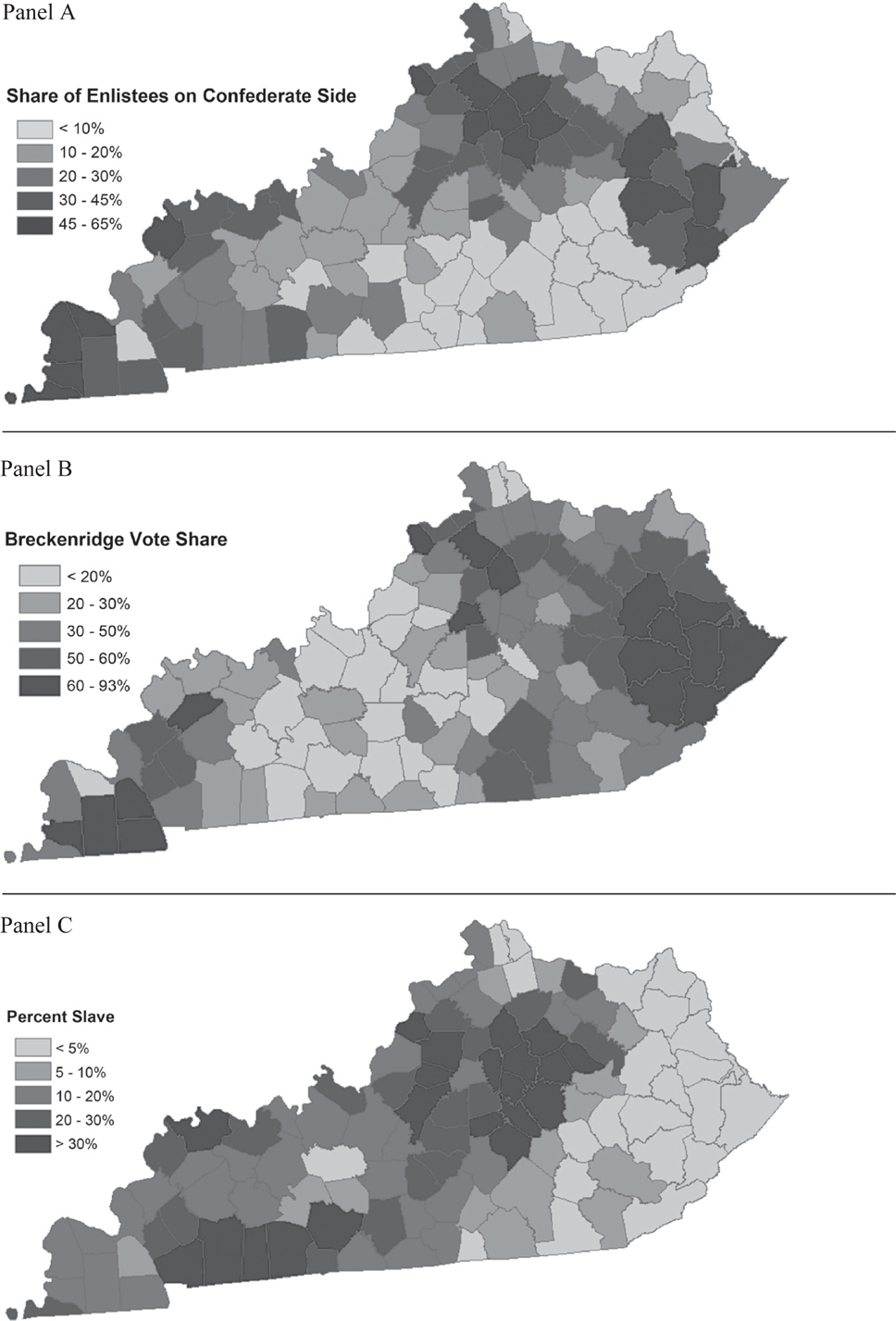
Figure 2 Kentucky County Characteristics
Data
Military Records
We begin with the collection of military records from the genealogical website fold3.com (U.S. War Department, 1890–1912), which we match to both the 1860 and 1880 censuses.Footnote 4 The military records are indexes to compiled service records, which include muster rolls and other documents collected from the War Department and the Treasury Department. These records exist for both Union and Confederate soldiers; however, they are likely more complete for Union soldiers. The indexes to these record collections contain the recruit’s regiment, full name, and (in some cases) age at enlistment. We extracted these indexes in their entirety for the state of Kentucky, with 107,589 entries on the Union side and 50,304 entries on the Confederate side.
Table 1 contains an illustration of the nature of the data from these indexes. An important complication with using these indexes is that it is not clear when multiple entries refer to the same person. The first three entries in Table 1 are men from the 3rd Union Cavalry named John Ewbanks, John Ubanks, and John Ebanks, respectively. The fourth entry is a man from the 55th Union Infantry, who is also named John Ewbanks. These names are all phonetic variants of one another, and could potentially refer to the same person. Soldiers frequently re-enlisted in multiple units, and if their names were spelled differently on different muster rolls or were duplicated for some other reason, they would appear in this index multiple times.
Table 1 Military Data: Example
Note: The table shows an illustration of possible groupings of military records, under different assumptions about which records constitute a single person. In panel A, we assume that all records with phonetically matching first and last names from the same regiment refer to the same individual. In panel B, we assume that all records with phonetically matching first and last names from the same side (Union or Confederate) refer to the same person. In panel C, we illustrate the “individuals” who constitute our final sample of military records, obtained from the genealogical website Fold3. com, which we link to the census of 1860. These consist of phonetic first and last names that appear uniquely on the Union or Confederate side, excluding records with first initials only.
Source: Example constructed by authors.
These duplicates pose a challenge for establishing the coverage of these records or the fraction of all enlistees who appear in the indexes. In particular, estimating the coverage of these indexes will depend on assumptions that we make about which records are duplicates. In the top panel of Table 1, we illustrate the least conservative grouping, in which we assume that phonetically identical names from the same regiment are the same person. In the example in Table 1, this assumption reduces the number of unique soldiers from ten to seven. In the entire sample, it reduces the number of unique soldiers to 78,257 Union and 37,917 Confederate, for a total of 116,174 recruits from Kentucky (see Table 2 for relevant statistics).Footnote 5 Another possibility is to assume that all Union or Confederate soldiers with phonetically identical names are the same person, as illustrated in panel B of Table 1; this assumption reduces the number of soldiers in Table 1 to 5, and it reduces the number of records in the complete sample to 64,309 (44,976 Union and 19,333 Confederate).
Table 2 Military Data: Summary Statistics
Note: Statistics pertaining to military records. Phonetic groups defined using NYSIIS codes. Approximately 75 percent of phonetic groups contain a single entry. See text for details of matching procedures.
Source: Authors’ calculations using data from U.S. War Department (1890–1912) linked to the 1860 full count census.
How do these sample sizes compare with the likely number of military recruits from Kentucky? An estimated 90,000 to 100,000 Kentuckians enlisted on the Union side, while only 30,000 to 40,000 enlisted on the Confederate side. Thus, the most conservative estimate of the number of recruits included in these records implies a coverage rate of around 50 percent. This represents a conservative lower bound, however. It is likely that multiple men with similar names did enlist, implying a much higher coverage rate of up to 100 percent.
The military indexes give us very little information other than the name of the recruit and the side on which he enlisted. Therefore, we need to match these indexes to other records to characterize the men and their outcomes. A challenge is that the only information we can use to match military indexes to other records is first and last name. Although many enlistment records contain the recruit’s age at enlistment, this variable is substantially more common in Union records: more than 80 percent of Union records contain the recruit’s age at enlistment while only about 15 percent of Confederate records do. Accordingly, we cannot use age at enlistment to match records without introducing significant systematic differences in the accuracy of matches by Union or Confederate status. We discuss this issue further in the Online Appendix.
An additional complication is that we cannot be sure how many individuals are covered by each unique name entry. Importantly, some names appear on both Union and Confederate rosters. To construct a list of names to match to census records, we group names by phonetic first and last name, defined using NYSIIS codes (Atack and Bateman Reference Atack and Bateman1992), and military side, that is, Union or Confederate. We restrict the sample to phonetic name groups that are uniquely identifiable as Union or Confederate, and we treat each phonetic group as a single individual. We also omit name groups that only include first initials, as we do not have sufficient information from these initials to accurately link our observations to other records.Footnote 6 As an example, see panel C of Table 1, in which only two of the five unique phonetic name groups listed would be included in our sample. The restrictions that we set leave 49,180 unique phonetic name groups remaining to be matched, 38,318 of which are Union and 10,862 of which are Confederate.
We select this method of constructing our database with specific empirical questions in mind. We are interested in comparing the ex-ante characteristics and post-war outcomes of Union and Confederate soldiers. To do so, we first identify a sample of Union and Confederate recruits-to-be in 1860. When constructing this sample, we aim to strike a balance between two (potentially) competing objectives: (1) maximizing the accuracy of the Union or Confederate status assigned to individuals in our sample, and (2) minimizing differences in the accuracy of Union and Confederate status. Objective (1) reduces attenuation bias in our estimates; objective (2) reduces bias of unknown direction (see Online Appendix A for details). Selecting a sample of names whose phonetic variants do not appear on both sides will increase the accuracy of our assignment of Union or Confederate status. Because Confederate records are more likely to contain only first initials as compared to Union records, omitting records with first initials avoids introducing systematic differences in the accuracy of Union and Confederate status. While we believe these methodological choices best enable unbiased comparisons between Union and Confederate recruits, they introduce certain concerns that are worth mentioning. Specifically, they cause people with uncommon names (which is not significantly related to socioeconomic status in our sample) to be overrepresented, and they reduce the size of the Confederate sample.
Matches to the 1860 Census
We match our sample of uniquely Union and Confederate names to the 1860 census using records from Ancestry.com via the National Bureau of Economic Research. Again, our challenge is that the only linkable information we have in our military data is the soldier’s name. To facilitate matching to the census, we impose certain restrictions on our target sample of census records. First, because our sample of recruits comes from regiments of white males, we limit our search to white males in the census. A sample of Union Army veterans indicates that 99 percent of Union recruits were born between 1817 and 1847 (Fogel Reference Fogel2000). Assuming a similar age range in the Confederate Army, and allowing for some error in the reporting of ages, we further restrict our search of the 1860 census to men born between 1815 and 1850. Finally, we restrict the geographic area in which we search for these soldiers to Kentucky.
Restricting our target sample to individuals living in Kentucky in 1860 is intended to improve the accuracy of our matches. Given that our recruits enlisted in Kentucky regiments, it is overwhelmingly likely that they resided in Kentucky at the time of enlistment, which occurred between 1861 and 1865. Companies were typically organized locally, and regiments were named after the enlistees’ state of origin. Therefore, potential matches residing in Kentucky are more likely to be correct than potential matches residing elsewhere. In the Online Appendix, we formally test this conjecture, and we conclude that restricting our search to men living in Kentucky in 1860 lowers the rate of matching error relative to an expanded search.Footnote 7
We match military records to white men ages 10–45 residing in Kentucky (275,999 records in target sample). We match names by searching for exact phonetic first name and surname matches between the military records and the target census sample and then by comparing the similarity of the first and last names using the Jaro–Winkler algorithm (Ruggles, Genadek, Goeken, et al. 2017). We discard matches with a string similarity score of less than 0.9.Footnote 8 Here, matching phonetically is a necessary but not sufficient condition for two records to be linked. Our use of the Jaro–Winkler algorithm allows us to avoid the clear false positives obtained when a phonetic algorithm alone is used to match names (Bailey, Cole, Henderson, et al. Reference Bailey, Cole and Henderson2017).
In addition to accuracy, we are interested in the representativeness of the matched sample. For instance, it is possible that we disproportionately match individuals with certain characteristics. This is difficult to characterize without information about the traits of Kentucky recruits, which is sparse, particularly for Confederates.Footnote 9 The best we can do is to compare the age of Union recruits from our enlistment data with the age of those recruits we are able to find in the 1860 census. We plot these two age distributions in Online Appendix Figure A1; they are broadly similar.
The 1860 census allows us to observe each man’s place of residence, family composition, each family member’s occupation and literacy status, and the value of the family’s real and personal property. We assign an occupational class (white collar, farmer, skilled blue collar, unskilled laborer, no occupation) to each recruit and to the head of his household if the recruit is a child. We also assign 1950 occupational codes to each individual’s occupation (Ruggles, Genadek, Goeken, et al. 2017), and then assign a value of occupational income based on the 1900 occupational wage distribution with an imputed wage for farmers (Preston and Haines Reference Preston and Haines1991; Abramitzky, Boustan, and Eriksson 2012; Olivetti and Paserman Reference Olivetti and Paserman2015; Salisbury Reference Salisbury2014).Footnote 10 Lastly, we obtain information on slave-owner status by linking the 1860 population census to the 1860 slave schedules (Ancestry.com 2010; see the Online Appendix for details).
Matches to the 1880 Census
We match our recruits from the 1860 census (12,440 in total) to the 1880 complete count database from the North Atlantic Population Project (Ruggles, Genadek, Goeken, et al. 2017). Here we make use of the demographic information we obtain from the 1860 census in order to locate recruits in 1880. We search the entire 1880 census for records that exactly match our 1860 census records on birth state, phonetic first and last name codes, sex, and race. We restrict birth year in the 1880 census to be no more than three years before or after birth year in the 1860 census. Finally, we discard matches in which the index measuring the similarity of names across census records (using the Jaro–Winkler algorithm) is less than 0.9. These procedures approximately follow Steven Ruggles, Katie Genadek, Ronald Goeken, et al. (Reference Ruggles, Genadek and Goeken2017). Using this procedure, we are able to match uniquely 30 percent of our Union soldiers and 29 percent of our Confederate soldiers. This match rate is comparable to other studies that perform automated record linkages (Ferrie Reference Ferrie1996; Ruggles, Genadek, Goeken, et al. 2017; Abramitzky, Boustan, and Eriksson 2012).Footnote 11 We emphasize that this sample will only consist of recruits who survive to 1880.
In addition to linking our sample of recruits to the 1880 census, we link male relatives of recruits who are under the age of 45 in 1860. Male relatives are defined as men who are living in the same household as an individual linked to a military record, but who are not themselves linked to a military record. Being unlinked does not necessarily mean that these relatives are civilians, but they are less likely to have fought in the war than those linked to a military record. We link these men using an identical procedure to that used to link soldiers to 1880. We are able to identify 29,747 male relatives of recruits in the 1860 census, and we link 17 percent of these to the census of 1880 (the rate is similar for relatives of Union and Confederate soldiers). This linkage rate is substantially lower than the linkage rate among soldiers. The lower match rate can be explained by the fact that soldiers in our database have uncommon names by construction, so relatively few records are discarded because they can be linked to multiple records in the 1880 census.
The representativeness of our sample is again difficult to address, primarily because the 1880 census did not ask about veteran status. We know that certain 1860 characteristics predict being linked to the 1880; in particular, recruits who were born in certain southern states are more likely to be found. This outcome is likely due to these states having small populations, which increases the probability of a unique match. Age seems also to predict linkage to 1880: the youngest recruits are least likely to be linked. Socioeconomic status—as measured by slaveholding—does not significantly predict linkage to 1880, nor do most county characteristics.
Characteristics of Union and Confederate Recruits
Panel A of Figure 2 illustrates the fraction of recruits linked to each county that enlisted on the Confederate side. There were relatively more Union recruits in coal-producing areas of the state, specifically in the lower portion of the eastern mountains and coalfields, and in the western coalfields. There were relatively more Confederate enlistees from the northeastern agricultural region and around the Mississippi Plateau in the southwest portion of the state, which is also an agricultural region. There was also a concentration of Confederates in the eastern part of the state along the border with Virginia. In panels B and C of Figure 2, we plot the share of the vote in the 1860 presidential election to John C. Breckenridge and the fraction of the population that was enslaved in 1860, respectively. It is clear from this figure that Confederate enlistment is positively correlated with both of these characteristics.Footnote 12
In Table 3, we compare average characteristics of Union and Confederate soldiers using our sample of 12,440 men linked from the Kentucky military records to the 1860 census. Column 1 contains mean characteristics for all 275,999 white men in Kentucky between the ages of 10 and 45. Column 2 contains mean characteristics for Union soldiers, column 3 contains means for Confederates, and column 4 contains p-values from tests of equality of the mean characteristics of Union and Confederate soldiers. Column 5 contains results from an OLS regression of an indicator for Union status on all characteristics together, which is run on our sample of Union and Confederate recruits.
Table 3 Characteristics of Union and Confederate Soldiers, 1860

Asterisks in column 4 refer to significance of the coefficient on the 1860 characteristic in a univariate regression of Union status on that characteristic.
*** p<0.01
** p<0.05
* p<10
Notes: For county-level characteristics, standard errors are clustered at the county level. Column 5 contains results from an OLS regression of an indicator for Union status on all characteristics together, using the sample of 12,440 soldiers linked to the 1860 census, of which 11,505 were not missing information and could be included. This regression also clusters standard errors by county.
Sources: Authors’ calculations using data from U.S. War Department (1890–1912) linked to the 1860 full count census; slaveholding variables from 1860 slaves schedules (Ancestry.com 2010); county characteristics are taken from Haines and ICPSR (Reference Haines2010); election returns data are taken from Clubb, Flanigan, and Zingale (Reference Clubb, Flanigan and Zingale2006).
As a group, soldiers were younger and less likely to be married than the general population. They were also more likely to be native to Kentucky or to the United States. There are substantial differences between Union and Confederate soldiers’ average characteristics. Union soldiers were older, more likely to be married, and less likely to live with a parent, although these differences are not statistically significant in the regression in column 5. There are, however, clear and significant differences in nativity. Confederate enlistees were more likely to be born in Kentucky or in the South generally. Union soldiers were more likely to be born in the Northeast or Midwest and were twice as likely to be foreign born (7.7 percent versus 3.4 percent). Evidence also points to differential selection of Confederate soldiers on socioeconomic characteristics. Confederate soldiers systematically came from counties with more slaves, greater value of property per family, and more people employed in agriculture.
Many significant differences between enlistees concern slaveholding. We find that Confederate soldiers were significantly more likely to come from a slave-owning household (26 percent versus 10 percent). These findings are consistent with men who had greater ties to slavery being more likely to join the Confederate Army. We also find significant differences in voting patterns. Men who joined the Confederate Army tended to live in counties with a greater vote share going to the Southern Democratic Party in the 1860 presidential election. Conversely, Union soldiers came from counties more likely to vote for John Bell.
Table 4 contains additional summary statistics for our sample of soldiers who are matched to the 1880 census. This table includes average outcomes in 1880 as well as average 1860 characteristics that we collected by hand for this sample; namely, family wealth and occupational status.Footnote 13 These results are largely consistent with Table 3 in that they point to Confederate recruits being of higher socioeconomic status. The table also indicates systematic differences in locational outcomes for Union and Confederate soldiers. We explore these differences in detail later.
Table 4 Summary Statistics of Linked 1860–1880 Census Data

Asterisks indicate whether or not the difference in means between Union and Confederate recruits is significant.
*** p<0.01
** p<0.05
* p<10
Notes: Characteristics of veterans linked between the census of 1860 and the census of 1880. See text for details about the linking process. In panel B, we report parent’s occupational status for the 1,719 out of 3,693 recruits who live with their parents; we report the recruits’ own occupational status for the remaining recruits.
Source: Authors’ calculations based on data from the U.S. War Department (1890–1912) linked to the 1860 full count census and the 1880 full count census (Ruggles et al. 2017).
Empirical Approach
Our empirical approach seeks to characterize the relationship between ideology and migration for men who fought on different sides of the Civil War. We acknowledge that men who enlisted on different sides may have made different migration decisions even if the Civil War had not happened, as these men may have held different social and political beliefs ex ante. However, the war experience may have magnified existing tensions and made local sympathy for the Confederacy or Union more salient for former soldiers. We focus our analysis on ideology, as manifested in military allegiance, and subsequent migration decisions for men who were similar on observable characteristics and initial locations.
Spatial equilibrium models (Roback Reference Roback1982; Moretti Reference Moretti2011) provide a useful framework for investigating the impact of ideology on post-war migration. We can think of local sympathy with the side a veteran fought for as an “amenity” that has value. For example, community members may revere veterans from the side they sympathize with and shun veterans from the opposite side. This local ideology over, for instance, questions of slavery and race, is likely to affect the utility a veteran derives from living in a particular place. Following Enrico Moretti (2011), suppose that veteran i’s utility in place a depends on the veteran’s earnings (yia), the cost of living (ra), local amenities (Aia), and a random component capturing this veteran’s idiosyncratic preference for place a (eia). In particular, ${U_{ia}} = {y_{ia}} - {r_a} + {A_{ia}} + {e_{ia}}.$
Veteran i will prefer place a to place b if Uia > Uib, or if his idiosyncratic preference for a over b exceeds his systematic preference for b over a. This becomes more likely after a negative shock to the relative amenity value of b (Aib – Aia).
If a is the veteran’s home in 1860, this means that a decline in the relative amenity value in the veteran’s home increases the probability that the veteran will migrate after the war. This framework also implies that, conditional on migrating, veterans are more likely to choose locations in which the amenity value has increased due to the Civil War. Thus, Union veterans should be more likely to leave places more sympathetic to the Confederacy in favor of places less sympathetic to the Confederacy, while Confederate veterans should do the opposite.
While the theoretical effect of a locality’s alignment with the Confederacy on migration behavior is straightforward, the effect on wages or land values is less so. In a simple model in which amenity values are common to everyone, an increase in amenity values generates a positive labor supply shock, which should lower real wages. In our case, amenity values change differently for men from a particular side. Specifically, a locality that is sympathetic to the Confederacy should see net in-migration of Confederate veterans and net out-migration of Union veterans, leaving the overall change in labor supply unclear. If we allow that individuals have idiosyncratically different earnings in different places, and if veterans make decisions about the tradeoff between amenities and earnings, we should expect veterans to do worse economically in places where they perceive a higher amenity value. However, if amenities are related to productivity or individual earnings, which may be the case if there are economic returns to social cohesion, or if social alignment with one’s community is productivity enhancing, then this prediction becomes unclear.
In our empirical work, we test whether the propensity to leave a county depends differently on ideology for Union and Confederate recruits who were otherwise similar based on observable characteristics and initial location. We also test whether migrants from Union and Confederate sides sorted differentially into places more sympathetic to the South. Although our model does not make clear predictions on the economic implications of these moves, we close our analysis with an investigation into the possible returns associated with migration after the Civil War.
Measures of Local Ideology
We use three county-level measures of local sympathy for the Confederacy. First, we use the share of Civil War recruits in a given county that enlisted in the Confederate Army. Second, we use the county’s share of the presidential vote going to John C. Breckenridge, the southern Democratic candidate, in the 1860 election. Breckenridge carried all southern states in the 1860 presidential election and explicitly supported the westward expansion of slavery; therefore, we assume that counties that favored Breckenridge were more aligned with the South than the North. We find that, conditional on other characteristics, a 10 percentage point increase in vote share to Breckenridge is associated with a 6 percentage point increase in the probability of serving in the Confederate Army. This result is significant at the 1 percent level. Third, we use the fraction of a county’s population that is enslaved in 1860. A 10 percentage point increase in the fraction enslaved is associated with a 6.5 percentage point increase in the probability of joining the Confederate Army.
A county’s Confederate enlistment share is perhaps the clearest measure of that county’s sympathy with the Confederacy. However, because we measure enlistment share using our sample of soldiers linked to the 1860 census, it is likely measured with error. In particular, we cannot be sure that we are sampling Union and Confederate soldiers from every county at the same rate. Moreover, this measure embeds a certain amount of linkage error. As an indicator of public opinion, Breckenridge vote share is likely measured with less error. However, the link between voting behavior and Confederate sympathy may be more tenuous than the link between Confederate enlistment and Confederate sympathy. The pre-war prevalence of slavery is likely a good indicator of Confederate sympathy; however, of our three measures, it is the most strongly correlated with the direct economic impact of the war. For instance, we know that Confederate recruits were more likely to be slave-owners than Union recruits. Thus, Confederate and Union recruits from counties in which slavery is prevalent may have experienced different wealth shocks following the Civil War, which may induce different migration behavior. As none of our measures is perfect, we present results using all three.
Migration Propensity
To determine whether Union recruits were more likely to leave more Confederate-leaning counties after the war, we estimate the following equation using OLS: ${M_{ij,1880}} = \alpha + {\beta _1}{U_{ij}} + {\beta _2}{U_{ij}} \times {S_{j,1860}} + \gamma {X_{i,1860}} + {\delta _j} + {u_{ij}}.$
Here, Mij is an indicator equal to one if person i from county j had migrated by 1880; Uij is equal to 1 if this person served in the Union Army; Sj,1860 is a measure of sympathy for the Confederacy in county j in 1860; Xi,1860 is a matrix of individual characteristics observed in 1860, including age and birthplace fixed effects; δj is an 1860 county fixed effect. We expect to find β 2 > 0.
A complication with this approach is that Union and Confederate recruits tended to have different occupations ex ante: Confederate recruits were more likely to hold skilled occupations in 1860. Thus, we may find that Union recruits were more likely to leave Confederate-leaning counties if these counties were more complementary to skilled individuals. In other words, differences in migration propensities may work through differences in individual skill and not differences in local ideology. Because we observe indicators of recruits’ socioeconomic status in 1860—namely, occupation (or occupation of the household head in the case of children), family wealth, literacy, and slave owner status—we can include interactions between ex ante socioeconomic status and our indicator of social alignment with the Confederacy. If β 2 is robust to the inclusion of these controls, then selection on skill is unlikely to fully explain differential migration behavior by military side.
It is also possible that Union and Confederate recruits were selected differently on unobservable skill, so controlling for 1860 socioeconomic status is not sufficient to show that differential migration behavior was associated with local ideology and not skill. One way to address this problem is to use recruits’ family members to control for systematic unobserved skill differences by military side. In addition to our sample of recruits, we link male family members of recruits, who are under the age of 45, to the 1880 census. We then estimate the difference in the difference in migration propensity between a soldier and his relative by military side. Specifically, we estimate the following: ${M_{ijk,1880}} = \alpha + {\beta _1}{V_{ijk}} + {\beta _2}{V_{ijk}} \times U{F_{jk}} + {\beta _3}U{F_{jk}} \times {S_{j,1860}} + {\beta _4}{V_{ijk}} \times {S_{j,1860}} + {\beta _5}{V_{ijk}} \times U{F_{jk}} \times {S_{j,1860}} + \gamma {X_{i,1860}} + {\delta _j} + {\phi _k} + {u_{ij}}.$
Variables are generally defined as i indexing individuals, j indexing county of origin, and k indexing families. The variable Vijk is equal to one if person i from county j and family k is a known soldier, and zero if this person is a known soldier’s family member. The indicator UFjk is equal to one if family k from county j is a “Union family” and zero otherwise. The parameter φk is a family fixed effect. For Confederate families, the difference between the marginal effect of Sj,1860 on the probability of migrating for veterans and their family members is β 4; for Union families, this difference in marginal effect is β 4 + β 5. The parameter we are most interested in is β 5: if β 5 > 0, this means that Union soldiers respond more to Sj,1860 than their family members, and by a greater margin than Confederate soldiers relative to their family members. The family fixed effect ensures that between-family variation in skill is not driving the result.
We note that, while β 5 > 0 is evidence that between-family skill is not the sole driver of differential migration behavior among Union and Confederate veterans, β 5 = 0 is not sufficient to prove that it is. If soldiers and soldiers’ family members were treated similarly after the war, then family members should have been equally encouraged to leave counties hostile to their side. Thus, even if ideology (and not skill) drove migration, we could observe that β 4 = β 5 = 0. Thus, in addition to arguing that ideology guides migration decisions, β 5 > 0 informs us about the way in which these forces work. In particular, β 5 > 0 indicates that ideology was more powerful for combatants than non-combatants.
Migration Destination
We study migration destinations for both individuals who departed Kentucky and those who left their home county but remained in the state. To determine whether Union recruits were more likely to sort into less Confederate-leaning counties within Kentucky, we estimate the following, using a sample of internal migrants: ${S_{il,1860}} = \alpha + \beta {U_{ijl}} + \gamma {X_{i,1860}} + {\delta _j} + {u_{ij}}.$
Here, Sil,1860 is a measure of social alignment with the Confederacy in 1860 in county l, where person i is residing in 1880; and Uijl is an indicator equal to one if person i who migrated from county j to county l between 1860 and 1880 served in the Union Army. The remaining variables are defined earlier. We expect to find β < 0, that is, Union veterans were less likely to migrate to counties with greater Confederate sympathy.
To determine whether Union recruits were more likely to move to different regions of the United States, we also estimate a multinomial logit model of residence in each region in 1880 on a sample of interstate migrants. We predict that Union veterans should be more likely to move to Union states in the Northeast and Midwest than enlistees on the Confederate side.Footnote 14 This analysis is again complicated by systematic differences in skill between Union and Confederate recruits. Because we are able to control for ex ante occupational attainment and family wealth, we can rule out the hypothesis that differences in locational choices are entirely driven by observable skill. We can also use non-veteran family members to control for family-specific unobservable skill.
Differences in Gains from Migration
Finally, we ask whether there were economic gains associated with differential migration by side after the Civil War. Our first measure is occupational income, or the average income in a particular occupation, which we estimate using the 1900 occupational wage distribution assigned to 1950 occupational codes (Preston and Haines Reference Preston and Haines1991; Abramitzky, Boustan and Eriksson 2012; Olivetti and Paserman Reference Olivetti and Paserman2015; Salisbury Reference Salisbury2014).Footnote 15 By using a national occupational income measure, we abstract away from migration returns experienced by moving to a place with a higher wage in a given occupation. In particular, the majority of our sample is comprised of farmers, who have the same occupational income regardless of where they live, despite large variation in actual income. We thus also use the value of agricultural output in a destination county to measure potential economic returns associated with moving. Our measure is the value of agricultural output per acre of farmland (improved and unimproved) in the 1880 county of residence (Haines and ICPSR Reference Haines2010).
We estimate the following by OLS: ${Y_{i,1880}} = \alpha + {\beta _1}{U_i} + {\beta _2}{M_{i,1880}} + {\beta _3}{M_{i,1880}} \times {U_j} + \gamma {X_{i,1860}} + {\delta _j} + {u_{ij}}.$
Variables are defined earlier, with Y i,1880 representing the economic outcome of interest in 1880. If β 3 > 0, then Union veterans experience a larger return to migration than Confederate veterans.
Results
Migration Propensity
We present results using our sample of soldiers’ names that are matched uniquely to Kentucky in 1860 (12,440 individuals). We are able to uniquely match 3,693 of these men to the 1880 census, in addition to 5,064 male family members (age 45 or younger) of our 12,440 soldiers in 1860. From Table 4, we can see that roughly 70 percent of our sample still resided in Kentucky as of 1880; however, approximately 50 percent of our sample had moved between counties by 1880. This is true of both Union and Confederate veterans. As can be seen in column 1 of Table 5, Union soldiers were no more or less likely to migrate than Confederate soldiers. However, migrants appear to be negatively selected from the overall population of Kentucky soldiers in terms of family wealth in 1860.
Table 5 Impact of County Characteristics on Migration Propensity

Note: “Union soldier” is an indicator for Union status in columns 1–3 and an interaction between an indicator for Union family status and veteran status in columns 4–5. Confederate enlistment share is the fraction of all soldiers linked to a particular county (12,440 soldiers in total) that are Confederate. Breckenridge vote share comes from Clubb, Flanigan, and Zingale (Reference Clubb, Flanigan and Zingale2006). County percent slave is from Haines and ICPSR (Reference Haines2010). All regressions contain controls for age (fixed effects in columns 1–3, quadratic in columns 4–5), birthplace fixed effects, and 1860 county of residence fixed effects. Column 3 also includes 1860 SES indicators (occupational class indicators for both the veteran and the household head; log(1+W), where W is the sum of family real and personal property; literacy; and an indicator for family slave owner status) and interactions between all SES indicators and county Confederate enlistment or Breckenridge vote share or percent slave. Column 5 contains family fixed effects and includes 1,372 families with more than one individual linked between 1860 and 1880. Standard errors are clustered at the 1860 county level.
Source: Authors’ calculations based on data from the U.S. War Department (1890–1912) linked to the 1860 full count census and the 1880 full count census (Ruggles et al. 2017).
In Table 5, we estimate the impact of the home county Confederate enlistment share (panel A), Breckenridge vote share (panel B), and fraction enslaved (panel C) on the propensity to migrate among Union and Confederate recruits (see equation (1)). The key variable is the interaction between Union soldier and our measure of alignment with the South: In column 2 of panel A, the coefficient can be interpreted to mean that the marginal effect of Confederate enlistment share on the probability of migrating is 0.419 (0.145) greater for Union soldiers than Confederate soldiers. Our results are qualitatively similar when we use Breckenridge vote share or the fraction enslaved to instead measure social alignment with the Confederacy (panels B and C of Table 5). To address concerns that this differential is driven by county-level differences in the return to skill, we include 1860 socioeconomic indicators (log family wealth, own and household head occupational class indicators, literacy, and household slave-owner status) and interactions between these variables and Confederate measures in column 3. The inclusion of these variables has a moderate impact on our results: the coefficient on the interaction between Union soldier and social alignment with the Confederacy decreases somewhat, and it is not quite significant at the 10 percent level when we use Breckenridge vote share; however, the coefficient remains large, positive, and significant when we use Confederate enlistment share and fraction enslaved.
To better understand the magnitude of our findings, we include a graphical representation in Figure 3. In panel A, we plot the predicted probability of migrating (based on results in column 3 of Table 5) for Union and Confederate soldiers with mean characteristics in a county with 5 percent Confederate enlistment share and in a county with 65 percent Confederate enlistment share (the maximum in our sample). The probability of a Confederate soldier leaving a county with 5 percent Confederate enlistment share is approximately 10 percentage points higher than the probability of an otherwise identical Union soldier leaving; however, the probability of a Confederate soldier leaving a county with 65 percent Confederate enlistment share is almost 15 percentage points lower than the probability of Union soldier leaving.

Figure 3 Impact of County Confederate Enlistment Share on Migration Propensity
In columns 4 and 5 of Table 5, we estimate equation (2), in which we use non-recruit family members to control for differences in unobservable skill by military side. In column 4, we omit family fixed effects and include UFjk (the indicator for Union family) as an explicit control. This specification allows us to include all linked soldiers and family members, not just pairs of soldiers and relatives from the same family. The necessary assumption here is that the distribution of unobservable skill is the same among Union veterans and Union family members. Similarly, the distribution of skill must be the same among Confederate veterans and Confederate family members. In these columns, the variable “Union soldier” is the interaction UF × V, which appears in equation (2). The key variable is the interaction between Union soldier and Sj,1860: in column 4 of panel A, the interpretation is that the difference in the marginal effect of Confederate enlistment share on the probability of migrating between soldiers and their family members is 0.330 (0.167) higher for Union than Confederate families. In column 5, in which we include family fixed effects, the coefficient is about twice as large. This result tells us two things: first, the different response to Confederate enlistment share by military side cannot be explained entirely by between-family differences in skill; second, former soldiers appear more responsive to local ideology than their relatives. The results in panels B and C are similar, albeit less conclusive. We perform additional robustness tests on the earlier findings in Online Appendix Tables A2, A3, and A4.
We illustrate these results graphically in panel B of Figure 3, which is based on our results from column 4 of Table 5. In a county with a 5 percent Confederate enlistment share, Union soldiers and family members are equally likely to leave, while Confederate soldiers are almost 10 percentage points more likely than their relatives to leave. Conversely, in a county with a 65 percent Confederate enlistment share, Union soldiers are around 5 percentage points more likely than their relatives to migrate, while Confederate soldiers are approximately 5 percentage points less likely to leave than their relatives.
Migration Destination
In Figure 4, we map the locations of Kentucky veterans who left Kentucky by 1880. There appear to be clear locational differences: Union recruits were more likely to move north, and Confederate recruits were more likely to move south and west. In Table 6, we estimate differences in regional locational choices of migrants by military side using a multinomial logit model of region of residence in 1880 (South, West, or Northeast, relative to the Midwest). Our explanatory variables include an indicator for having served in the Union Army, as well as other 1860 characteristics including age, birthplace, and county of residence fixed effects. We find that Union recruits were significantly more likely to migrate to the Midwest than either the South or the West. In particular, the odds of moving to the South relative to the Midwest for Union veterans are roughly three-quarters the relative odds of moving to the South for former Confederates. This result is robust to controlling for ex-ante occupational attainment and family wealth (column 2), so differences in destination region cannot be explained by differences in observable skill.Footnote 16

Figure 4 Distribution of Migrants From Union and Confederate Armies, 1880
Table 6 Locational Choices of Migrants: Multinomial Logit Model of 1880 Region of Residence

Note: “Union soldier” is an indicator for Union status in columns 1–3 and an interaction between an indicator for Union family status and veteran status in column 4. Null results about the impact of military side on the probability of migrating to the Northeast (relative to the Midwest) are omitted for brevity. Controls for 1860 SES include own and household head occupational class indicators, log family wealth, literacy, and family slave-owner status (see notes to Table 5 for details). Controls for the value per acre of agricultural land and the farm ownership rate in 1880 are from Haines and ICPSR (Reference Haines2010). See the text for a discussion of why we include the 1880 variables as controls in some specifications.
Source: Authors’ calculations based on data from the U.S. War Department (1890–1912) linked to the 1860 full count census and the 1880 full count census (Ruggles et al. 2017).
The Homestead Act of 1862 may have influenced the migration choices of veterans differentially and generated the disparities in destination region we find. For the first five years of the program, which allowed men to apply for ownership of plots of land in the Midwest, Confederate veterans were excluded.Footnote 17 They were later allowed to participate along with Union veterans, and the majority of early homesteaders staked out land in Missouri, Iowa, Michigan, Wisconsin, and Minnesota. Union veterans’ early access to these plots seems unlikely to be driving our results, however. While almost 16 percent of Union veterans who left Kentucky moved to Missouri, very few went to the other popular homesteading states. In fact, almost 40 percent of Union men who left Kentucky moved to Illinois, Indiana, and Ohio, which were states with few homesteading applications. Meanwhile, we observe that Confederate migrants also commonly moved to Illinois, Indiana, or Missouri; however, the remainder were more likely to choose states in the South and far West.
To further explore the potential role of Union veterans’ preferential access to the Homestead Act, we control for two salient 1880 county characteristics: average farm value per acre, and the ownership rate in agriculture. These county characteristics are themselves outcomes; as such, this is certainly not our preferred specification. It is merely a test of the hypothesis that differences in destination region can be explained entirely by the fact that Union recruits were able to access better land under the Homestead Act. If this is the case, then including these controls should wipe out any systematic regional differences in location by military side. We show this is not the case, as can be seen in column 3 of Table 7. In column 4, we include non-recruit family members to address the possibility that Union and Confederate soldiers are differently selected on unobservable skill. Because we have very few linked soldier-relative pairs who are both migrants, we do not implement a family fixed effects model similar to equation (2). Rather, we include UFjk as a control and omit the family fixed effect. The results are very similar, although the impact of being a Union soldier on the probability of moving to the South (relative to the Midwest) is not quite significant at the 10 percent level.
Table 7 Locational Choices of Intrastate Migrants: Characteristics of 1880 County of Residence

Note: “Union soldier” is an indicator for Union status in columns 1–2 and an interaction between an indicator for Union family status and veteran status in column 3. Sample consists of individuals who left their county of origin for another county in Kentucky between 1860 and 1880; standard errors clustered by 1880 county. Controls for 1860 SES include own and household head occupational class indicators, log family wealth, literacy, and family slave-owner status. (see notes to Table 5 for details). Controls for the value per acre of agricultural land and the farm ownership rate in 1880 are from Haines and ICPSR (Reference Haines2010).
Source: Authors’ calculations based on data from the U.S. War Department (1890–1912) linked to the 1860 full count census and the 1880 full count census (Ruggles et al. 2017).
In Table 7, we estimate differences in destination county characteristics within Kentucky (equation (3)). We take a sample of men living in Kentucky in 1880, but in a different county from their county of residence in 1860. We regress the Confederate enlistment share (panel A), 1860 Breckenridge vote share (panel B), or the 1860 slavery rate (panel C) in the person’s 1880 county of residence on a Union indicator, adding the same controls as in Table 6. In columns 1 and 2, we find that Union soldiers who migrated within Kentucky were significantly less likely to end up in a county more sympathetic to the Confederacy. In column 3, we add non-combatant relatives. We find that internal Kentucky migrants from Union families were significantly less likely to end up in Confederate-sympathizing counties than those from Confederate families; however, there is not a significant differential effect for soldiers relative to their family members unless we measure Confederate sympathy by the slavery rate.
Differences in Gains from Migration
In Table 8 we explore the economic returns to post-Civil War migration for Union and Confederate soldiers. The Roback model we discuss in the Empirical Approach section does not provide strong predictions for theoretical wage impacts of migration associated with an ideological amenity, and we are limited by our data in the type of analysis we can pursue. In particular, the majority of our sample is comprised of farmers, so we do not have variation in occupational income for this group. Furthermore, many of the migrations we observe are within the state of Kentucky, and the previous literature has not suggested large economic returns associated with short-distance moves (Salisbury Reference Salisbury2014).Footnote 18 We thus view this portion of our analysis as relatively speculative.
Table 8 Differential Returns to Migration by Military Side

Note: Sample consists of soldiers only. See notes to Table 5 for variable definitions. All regressions include age, birthplace, and county of origin fixed effects. Standard errors in panel B are clustered by 1880 county of residence.
Source: Authors’ calculations based on data from the U.S. War Department (1890–1912) linked to the 1860 full count census and the 1880 full count census (Ruggles et al. 2017).
In panel A, we report differences in migration returns in terms of occupational income for our sample. In particular, we regress occupational income in 1880 on an indicator for the person having moved counties between 1860 and 1880, an indicator for serving in the Union Army, and an interaction between these two variables. We find that Union soldiers have poorer occupational outcomes than did Confederate soldiers, even conditional on the occupational income and wealth of the soldier’s household head in 1860. This finding may indicate that Confederate recruits were more positively selected than Union recruits on unobservables; or, it may indicate a positive causal effect of service in the Confederate Army relative to service in the Union Army. In any case, Union soldiers were unable to overcome their initial occupational disadvantage over the next two decades despite having emerged victorious in the conflict.
In columns 3 and 4, we include an indicator for having migrated out of a soldier’s home county in 1860. The coefficient on the main effect of migrating and the interaction between migrating and Union status are both close to zero and insignificant, indicating no return to migration in terms of occupational income for soldiers on either side. We note that our measure of occupational income obscures any gains to migrants who earned higher wages in their destination county despite remaining in the same occupation. It is thus possible that there was some economic return that we could capture using wage data; however, we consider this possibility unlikely because a majority of our sample is comprised of farmers.
In the bottom panel, we estimate the relationship between military side and the value of agricultural land in a veteran’s 1880 county of residence to explore whether veterans who moved may have experienced a benefit to doing so in farming. In columns 1 and 2, we see that, on average, Union and Confederate veterans lived in similar counties in terms of agricultural land value. However, this masks heterogeneity in agricultural land value by migrant status. We find that Union veterans who remained in their home counties lived in areas with systematically worse agricultural land than did Confederates, indicating that Unionists lived in places with lower farm value per acre ex ante (columns 3 and 4). However, our results suggest that Union veterans who migrated did so to places with better land than did otherwise similar Confederates. In particular, while Confederates moved to counties with farm values per acre that were 8 percent lower than where they lived originally, Union veterans moved to counties with values that were 17 percent higher (column 3). It turns out that much of this effect is driven by the fact that Union veterans were likely to move to the Midwest, where land values were higher. When we include fixed effects for 1880 region of residence (column 4), we find that the difference between land values for Union movers and stayers is still positive but not quite significant at the 10 percent level. So, the fact that Union recruits were disproportionately likely to move to the Midwest— which we argue is at least partly driven by ideology—may have had a real impact on the relative return to migration in farming.
Conclusion
Our results paint a complex portrait of the relationship between ideology and migration in the aftermath of the American Civil War. Union veterans from Kentucky were more likely to leave counties dominated by their ideological (and wartime) adversaries and move to places that had supported the Union. We cannot fully disentangle whether they moved to the Midwest because of the provisions of the Homestead Act or, if because of the Act, the newly opened areas would be largely devoid of Confederates. However, our results suggest that because of ideology and related institutions, the Civil War had differential impacts on Kentucky Confederates, who found their options for improving their circumstances by moving to be comparatively limited. Our results also suggest that Union veterans were better able to move to areas with more productive farmland in other states after the war than were Confederates.
More broadly, our findings suggest that animosity between Union and Confederate veterans had a real impact on their migration behavior during the post-bellum period, possibly limiting northern migration of southern whites despite large potential economic gains. Enduring ideological divisions should serve as a companion to other explanations for limited South-to-North migration during this period, such as information flows and path dependence. We concluded our empirical work by exploring the economic benefits to migrating for white veterans. However, it is also possible that ideological sorting imposed costs on black individuals left behind. In particular, the departure of Union veterans from Confederate-dominated parts of border states may have facilitated the rise of Jim Crow institutions in these areas (see Blight Reference Blight2001). Future research could explore this conjecture in more detail.