


1. Introduction: meager state of theoretical modelling of aerodynamics
The problem of the flow over a lifting airfoil is a century-old, classical textbook problem in aerodynamics and fluid mechanics (Karamcheti Reference Karamcheti1966; Schlichting & Truckenbrodt Reference Schlichting and Truckenbrodt1979; Milne-Thomson Reference Milne-Thomson1996). The problem is analytically solvable thanks to three elements. First, the potential flow around a circular cylinder is readily known since the 1877 seminal paper of Lord Rayleigh (Reference Rayleigh1877). Second, the Riemann mapping theorem (dating back to Riemann's PhD dissertation 1851) ensures that any simply connected domain can be (biholomorphically) mapped to the open disc. So, the flow around any two-dimensional shape can be easily constructed from the cylinder flow via conformal mapping between the cylinder and the shape of interest. However, this solution is not unique. One can always add a circulation of arbitrary strength at the centre of the cylinder, which does not affect the no-penetration boundary condition at all. Interestingly, this circulation is of paramount importance for lift production; in fact, it solely dictates the amount of lift generated. Therefore, the potential-flow theory alone cannot predict the generated lift force; a closure condition must be provided to fix the dynamically correct amount of circulation. The third element is the Kutta–Zhukovsky condition, which has traditionally provided such a closure.
The Kutta condition is quite intuitive: if the body has a sharp trailing edge leading to a singularity, then the circulation must be set to remove such a singularity; it is a singularity removal condition (Crighton Reference Crighton1985). It is quite accurate for a steady flow (at a high Reynolds number and a small angle of attack); indeed, it is a paradigm for engineering ingenuity where an enabling mathematical condition is inferred from physical observations.
Interestingly, if one wishes to consider a smooth trailing edge, however small the trailing radius (i.e. however close to a sharp trailing edge), the classical aerodynamic theory collapses; there are no theoretical models that can predict lift on a two-dimensional smooth body without sharp edges! (Only a few ad-hoc methods with no theoretical basis.) In fact, some authors even consider the sharp edge as a lifting mechanism; i.e. an airfoil must have a sharp trailing edge to generate lift (Hoffman, Jansson & Johnson Reference Hoffman, Jansson and Johnson2016).
For unsteady flows, the status of current aerodynamic theory is even worse. Kutta never claimed that his condition works for unsteady flows; in fact, for an unsteady case, it is already known that, in the early transient period after an impulsive start, the flow goes around the trailing edge from the lower surface to the upper surface (see Tietjens & Prandtl (Reference Tietjens and Prandtl1934), pp. 158–168; Goldstein (Reference Goldstein1938), pp. 26–36; Schlichting & Truckenbrodt (Reference Schlichting and Truckenbrodt1979), pp. 33–35). That is, since more than a century, it is known that the Kutta condition is not generally applicable to unsteady flows (even for airfoils with sharp trailing edges at small angles of attack). This is why numerous research reports have criticized the application of the Kutta condition to unsteady flows (Woolston & Castile Reference Woolston and Castile1951; Rott & George Reference Rott and George1955; Abramson & Chu Reference Abramson and Chu1959; Chu & Abramson Reference Chu and Abramson1959; Chu Reference Chu1961; Henry Reference Henry1961; Shen & Crimi Reference Shen and Crimi1965; Abramson, Chu & Irick Reference Abramson, Chu and Irick1967; Orszag & Crow Reference Orszag and Crow1970; Basu & Hancock Reference Basu and Hancock1978; Daniels Reference Daniels1978; Satyanarayana & Davis Reference Satyanarayana and Davis1978; Savage, Newman & Wong Reference Savage, Newman and Wong1979; Bass, Johnson & Unruh Reference Bass, Johnson and Unruh1982; Crighton Reference Crighton1985), including the recent efforts of Xia & Mohseni (Reference Xia and Mohseni2017), Taha & Rezaei (Reference Taha and Rezaei2019) and Zhu et al. (Reference Zhu, McCrink, Bons and Gregory2020) among others. Nevertheless, almost all unsteady models, starting with the pioneering efforts in the 1920s and 1930s of Wagner (Reference Wagner1925), Theodorsen (Reference Theodorsen1935) and Von Kármán & Sears (Reference Von Kármán and Sears1938) until the recent work of Baddoo, Hajian & Jaworski (Reference Baddoo, Hajian and Jaworski2021), adopted the Kutta condition. There is no legitimate alternative! So, what we have is a meager state of knowledge and a very confined capability of aerodynamic theoretical modelling: we can only analyse steady flow at a small angle on a body with a sharp trailing edge! Basically, the aerodynamic theory is encumbered with the Kutta condition; it is applicable whenever the latter is befitting. It is clear that we lack a general theory for lift computation – equivalently a general closure principle, alternative to Kutta's, for potential flow.
The above discussion is intimately related to the lifting mechanism. The accepted wisdom by the fluid mechanics community asserts that the Kutta condition is a manifestation of viscous effects – it implicitly accounts for viscous effects in a potential-flow formulation. In fact, this view has been challenged by several authors (Hoffren Reference Hoffren2000; Hoffman et al. Reference Hoffman, Jansson and Johnson2016), but without providing a mathematical proof or theoretical basis. It may be the right time to recall Chang's 2003 New York Times article: What Does Keep Them Up There? (Chang Reference Chang2003): ‘To those who fear flying, it is probably disconcerting that physicists and aeronautical engineers still passionately debate the fundamental issue underlying this endeavour: what keeps planes in the air?’.
In this paper we revive a special variational principle from the history of analytical mechanics: Hertz’ principle of least curvature. Exploiting such a variational principle, we develop a novel variational formulation of Euler's equations for the dynamics of ideal fluids where the Appellian (integral of squared acceleration) is minimized. The new variational formulation is fundamentally different from the several developments based on Hamilton's principle of least action (Hargreaves Reference Hargreaves1908; Bateman Reference Bateman1929; Herivel Reference Herivel1955; Serrin Reference Serrin1959; Penfield Reference Penfield1966; Luke Reference Luke1967; Seliger & Whitham Reference Seliger and Whitham1968; Bretherton Reference Bretherton1970; Salmon Reference Salmon1988; Loffredo Reference Loffredo1989). It even transcends Euler's equation in some singular cases where the latter does not provide a unique solution, such as the airfoil problem.
Applying the developed variational formulation to the century-old problem of the flow over an airfoil, we develop a new variational theory of lift that dispenses with the Kutta condition. The Hertz principle of least curvature is used, as a first principle, to develop, for the first time, a closure condition alternative to Kutta's for the potential flow over an airfoil. In contrast to the Kutta condition, the developed closure condition is derived from first principles. The new variational condition reduces to the Kutta condition in the special case of a sharp-edged airfoil, which challenges the accepted wisdom about the Kutta condition being a manifestation of viscous effects. Rather, it is found that the Kutta condition is a momentum conservation mechanism for the inviscid flow over a sharp-edged airfoil. Moreover, the developed theory, unlike the classical theory, allows treatment of smooth, singularity-free shapes. Using this new theory, we resolve the seeming contradiction between various results in literature about the lifting capability of superfluids. We provide conditions on the geometry of the body to generate lift in a superfluid.
2. Lack of dynamical features in the current theory of aerodynamics: variational formulation is the panacea
To solve for the flow field of an incompressible fluid, both the continuity (kinematics) and momentum (dynamics) equations must be solved simultaneously. However, in potential flow the governing equation is the Laplacian in the velocity potential ( $\nabla ^2\phi =0$), which is obtained by combining the continuity equation (a divergence-free constraint: ${\boldsymbol {\nabla } \boldsymbol {\cdot }\boldsymbol {u}=0}$) with an irrotational-flow assumption (a curl-free constraint: $\boldsymbol {\nabla }\times \boldsymbol {u}=0$). These are kinematic constraints on the velocity field $\boldsymbol {u}$. Then, the momentum equation (Bernoulli's in this case) is considered next to solve for the pressure field. That is, in potential flow the flow kinematics is decoupled from the flow dynamics; the velocity field is determined from purely kinematic analysis without any consideration for dynamical aspects. Therefore, it is fair to expect that such a pure kinematic analysis is not sufficient to uniquely determine the flow field. Hence, the fix must come from a dynamical consideration. Note that this is not the case for three-dimensional flows because the domain enclosing a three-dimensional surface is simply connected while that around a two-dimensional object is doubly connected: a closed circuit around the three-dimensional surface is a reducible circuit while that around a two-dimensional object is irreducible; there is no means to determine the circulation of an irrotational flow around an irreducible circuit in a doubly connected region (Karamcheti Reference Karamcheti1966, pp. 259–260).
It may be interesting to point out that the circulation is actually a dynamical quantity; it is directly related to the lift force (i.e. pressure distribution). This is consistent with the recent effort of Hemati, Eldredge & Speyer (Reference Hemati, Eldredge and Speyer2014) who showed that when a potential-flow solver is fed with measurements of the total lift force, the resulting potential-flow field is quite close to the actual flow field even at unsteady high-angle-of-attack situations. However, the generated lift forces are essentially unknowns, in fact, the primary unknowns of interest to an aerodynamicist.
Based on the above discussion, a proper closure condition (i.e. a condition that provides circulation dynamics) in potential flow must come from dynamical considerations. The challenge is: Can we project Euler's dynamical equations on a one-dimensional manifold to extract the dynamics of circulation alone?
Dynamical equations of motion can be determined either from a Newtonian mechanics perspective or an analytical mechanics one. The former stipulates isolating fluid particles and writing equations of motion for each individual particle even if the free variables in the system are significantly fewer than the total number of spatial coordinates of all individual particles due to kinematic or geometric constraints. For example, let us assume a simple mechanics problem of 100 particles in the plane (i.e. 200 degrees of freedom for the particles), but are rigidly connected (i.e. subject to kinematic constraints) in some way that leaves only three free variables ( $q_1$, $q_2$, $q_3$), as shown in the schematic of figure 1(a). That is, given these three variables at any time instant, one can construct the motion of all 100 particles. The Newtonian approach requires writing down 200 equations of motion ( $m_i\boldsymbol {a}_i=\boldsymbol {F}_i+\boldsymbol {R}_i,\ i=1,\ldots,100$) even though only three are relevant for the motion. In addition, because the Newtonian approach requires separating each particle from the surrounding, as shown in the free body diagram in figure 1(b), the unknown constraint forces $\boldsymbol {R}_i$ appear, which compels the dynamicist to explicitly consider the 197 constraint forces $\boldsymbol {R}_i$ (i.e. forces that maintain the kinematical constraints) even though these forces are workless (i.e. do not contribute to the motion per se). On the other hand, the analytical (Lagrangian or variational) mechanics approach allows accepting the kinematical constraints, ignoring the unknown forces that maintain them, and hence focusing on the relevant equations of motion; it provides directly the relevant equations of motion for the free variables by minimizing a certain objective function, called the action $\mathcal {A}$. That is, the first derivative of the action with respect to each variable must vanish; i.e. we have ${\partial \mathcal {A}}/{\partial q_j}=0$, $j=1,2,3,$ in the considered example.

Figure 1. A schematic diagram for 100 particles in the plane that are rigidly connected such that only three degrees of freedom  $q_1$, $q_2$, $q_3$ are left, along with the free body diagram of the $i$th particle. Here $\boldsymbol {F}_i$ is an applied/impressed force whereas $\boldsymbol {R}_i$ is a constraint force whose sole role is to maintain kinematic constraints. (a) Schematic of 100 rigidly connected particles, (b) free body diagram of the $i$th particle.
Projecting this discussion on the potential-flow case, one finds that the kinematical constraints of potential flow allow construction of the entire flow field  $\boldsymbol {u}$ from the circulation free variable $\varGamma$ only: $\boldsymbol {u}=\boldsymbol {u}(\boldsymbol {x};\varGamma )$. That is, while there are infinite degrees of freedom for the infinite fluid particles, there is only one free variable (the circulation) which, via the potential-flow kinematical constraints, can be used to recover the motion of these infinite degrees of freedom. Hence, the analytical/variational mechanics appears to be specially well suited for this problem; it will provide a single equation for the unknown circulation without paying attention to the irrelevant degrees of freedom of the fluid particles or the unknown forces that maintain kinematical constraints. Simply, the first variation of the action with respect to circulation must vanish – and this necessary condition should provide a single dynamical equation in the unknown circulation: ${\partial \mathcal {A}}/{\partial \varGamma }=0$.
Based on the above discussion, two important conclusions are drawn: (i) a true closure/auxiliary condition for potential flow must come from dynamical considerations, and (ii) variational principles would be particularly useful to derive such dynamics. Insofar as this story looks appealing, the questions have always been as follows. What is a suitable variational principle for the airfoil problem? What is the special quantity that is being minimized in every attached flow over a body?
3. Theoretical mechanics approach: Gauss’ principle of least constraint and Hertz’ principle of least curvature
There have been several variational formulations of Euler's equations; almost all of them are based on Hamilton's principle of least action (Hargreaves Reference Hargreaves1908; Bateman Reference Bateman1929; Herivel Reference Herivel1955; Serrin Reference Serrin1959; Penfield Reference Penfield1966; Luke Reference Luke1967; Seliger & Whitham Reference Seliger and Whitham1968; Bretherton Reference Bretherton1970; Salmon Reference Salmon1988; Loffredo Reference Loffredo1989). However, Hamilton's principle suffers from some drawbacks that precludes its applicability to the airfoil problem. In particular, Hamilton's principle is a time-integral variational principle. That is, the quantity that is being extremized is an integral over time; hence, it may not be applicable to a steady snapshot of a flow field without the need to trace the evolution of the flow during its transient towards the steady equilibrium. Also, Hamilton's principle is exactly equivalent to Lagrange's (and Newton's) equations, so it does not provide more information in the singular cases where Lagrangian (and Newtonian) mechanics fail to determine a unique solution.
In fact, the search for a suitable variational formulation for the airfoil problem is challenging. For example, minimizing the kinetic energy over the field yields trivial (zero circulation) at any angle of attack. We found that the deserted principle of least constraint by Gauss provides a felicitous formulation for the current problem. In fact, Gauss' principle seems to have gone into oblivion in the history of mechanics. Papastavridis wrote: ‘In most of the 20th century English literature, GP [Gauss Principle] has been barely tolerated as a clever but essentially useless academic curiosity, when it was mentioned at all’ (Papastavridis Reference Papastavridis2014, p. 924).
Consider the dynamics of  $N$ particles, each of mass $m_i$, which are governed by Newton's equations
 \begin{equation} m_i \boldsymbol{a}_i = \boldsymbol{F}_i + \boldsymbol{R}_i \quad \forall\ i\in\{1,\ldots,N\}, \end{equation}
where  $\boldsymbol {a}_i$ is the inertial acceleration of the $i$th particle, and the right-hand side represents the total force acting on the particle, which is typically decomposed in analytical mechanics into (i) impressed forces $\boldsymbol {F}_i$, which are the directly applied (driving) forces (e.g. gravity, elastic, viscous); and (ii) constraint forces $\boldsymbol {R_i}$ whose raison d'etre is to maintain/satisfy kinematical/geometrical constraints; they are passive or workless forces (Lanczos Reference Lanczos1970). (For time-varying constraints, only the virtual work of the constraint forces vanishes, but not necessarily their actual work (Papastavridis Reference Papastavridis2014, pp. 382–383).) That is, constraint forces do not contribute to the motion abiding by the constraint; their sole role is to preserve the constraint (i.e. prevent any deviation from it).
Inspired by his method of least squares, Gauss (Reference Gauß1829) asserted that the deviation of the actual motion  $\boldsymbol {a}$ from the impressed one ${\boldsymbol {F}}/{m}$ is minimum. That is, the quantity
 \begin{equation} \mathcal{A} = \sum_{i=1}^N \frac{1}{2} m_i\left( \frac{\boldsymbol{F}_i}{m_i} - \boldsymbol{a}_i \right)^2 \end{equation}
is minimum (Papastavridis Reference Papastavridis2014, pp. 911–912). Several points are worthy of clarification here. First, Gauss’ principle is equivalent to (derivable from) Lagrange's equations of motion (Papastavridis Reference Papastavridis2014, pp. 913–925), so we emphasize that it bears the same truth and status of first principles (Newton's equations). Second, in Gauss’ principle,  $\mathcal {A}$ is actually minimum, not just stationary. Third, unlike the time-integral principle of least action, Gauss’ principle is applied instantaneously (at each point in time). So, it can be applied to a particular snapshot. Fourth, in some of the singular cases (when the dimension of the tangent space changes), Newtonian and Lagrangian mechanics (as well as the principle of least action) may fail to determine a unique solution. In contrast, Gauss’ principle is capable of providing a unique solution (see Papastavridis (Reference Papastavridis2014), p. 923; and Golomb (Reference Golomb1961), pp. 71–72).
In the case of no impressed forces
 \begin{equation} m_i \boldsymbol{a}_i = \boldsymbol{R}_i \quad \forall\ i\in\{1,\ldots,N\}, \end{equation}
Gauss’ principle reduces to Hertz’ principle of least curvature, which states that the Appellian
 \begin{equation} S = \sum_{i=1}^N \frac{1}{2}m_i\boldsymbol{a}_i^2 \end{equation}
is minimum, where  $\boldsymbol {a}_i^2=\boldsymbol {a}_i\boldsymbol {\cdot }\boldsymbol {a}_i$ is a scalar product. In this case, because kinetic energy is conserved, it can be shown that the system curvature (i.e. the instantaneous sum of curvatures of particles’ trajectories) is minimum (Papastavridis Reference Papastavridis2014, pp. 930–932). That is, a free (unforced) particle moves along a straight line. However, if it is a constrained motion, it will deviate from a straight line to satisfy the constraint, but the deviation from the straight line path (i.e. curvature) would be minimum.
4. Novel variational formulation of the dynamics of ideal fluids
Recall the Euler equations for incompressible flows
 \begin{equation} \rho\boldsymbol{a} ={-}\boldsymbol{\nabla} p,\quad {\rm in}\ \varOmega, \end{equation}
subject to continuity
 \begin{equation} \boldsymbol{\nabla} \boldsymbol{\cdot} \boldsymbol{u} = 0,\quad {\rm in}\ \varOmega, \end{equation}
and the no-penetration boundary condition
 \begin{equation} \boldsymbol{u}\boldsymbol{\cdot} \boldsymbol{n} = 0,\quad {\rm on}\ \partial{\varOmega}, \end{equation}
where  $\varOmega$ is the spatial domain, $\partial \varOmega$ is its boundary, $\boldsymbol {n}$ is normal to the boundary, and $\boldsymbol {a}={\partial \boldsymbol {u}}/{\partial t}+\boldsymbol {u}\boldsymbol {\cdot }\boldsymbol {\nabla } \boldsymbol {u}$ is the total acceleration of a fluid particle.
Equation (4.1) presents Newton's equations of motion for the fluid parcels. For inviscid flows, neglecting gravity, the only acting force on a fluid parcel is the pressure force  $\boldsymbol {\nabla } p$. In order to apply Gauss’ principle, we must determine whether this force is an impressed force or a constraint force. Interestingly, for incompressible flows, it is the latter. The sole role of the pressure force in incompressible flows is to maintain the continuity constraint: the divergence-free kinematic constraint on the velocity field ( $\boldsymbol {\nabla } \boldsymbol {\cdot } \boldsymbol {u} = 0$). It is straightforward to show that if $\boldsymbol {u}$ satisfies (4.2), (4.3), then (Kambe Reference Kambe2002, p. 261)
 \begin{equation} \int_\varOmega (\boldsymbol{\nabla} p \boldsymbol{\cdot} \boldsymbol{u})\,{\rm d}\kern0.06em \boldsymbol{x} =0 \end{equation}
for any scalar  $p$, which indicates that pressure forces are workless through divergence-free velocity fields that are parallel to the surface; i.e. satisfying (4.3). That is, if a velocity field satisfies continuity (i.e. divergence free) and the no-penetration boundary condition (4.3), the pressure force would not contribute to the dynamics of such a field. This fact is the main reason behind vanishing the pressure force in the first step in Chorin's standard projection method for incompressible flows (Chorin Reference Chorin1968); when the equation of motion is projected onto divergence-free fields, the pressure term disappears, which is based on the Helmholtz–Hodge decomposition (e.g. Kambe Reference Kambe2002; Wu, Ma & Zhou Reference Wu, Ma and Zhou2007): a vector $\boldsymbol {v}\in \mathbb {R}^3$ can be decomposed into a divergence-free component $\boldsymbol {u}$ that is parallel to the surface; i.e. satisfying (4.3), and a curl-free component $\boldsymbol {\nabla } f$ for some scalar function $f$ (i.e. $\boldsymbol {v}=\boldsymbol {u}+\boldsymbol {\nabla } f$). These two components are orthogonal as shown in (4.4).
From the above discussion, it is clear that the pressure force is a constraint force and the dynamics of ideal fluid parcels are subject to no impressed forces. (This will not be the case for a non-homogeneous, normal flow boundary condition.) Hence, Gauss’ principle of least constraint reduces to Hertz’ principle of least curvature in this case.
Considering the dynamics of an ideal fluid (4.1), and labelling fluid parcels with their Lagrangian coordinates  $\boldsymbol {\xi }$ (initial positions), we write the Appellian as
 \begin{equation} S = \int \frac{1}{2} \rho_0 \boldsymbol{a}^2 \,{\rm d}\boldsymbol{\xi}, \end{equation}
where  $\rho _0=\rho _0(\boldsymbol {\xi })$ is the initial density. Realizing that $\rho J = \rho _0$, where $J$ is the Jacobian of the flow map (Bateman Reference Bateman1929), the Appellian is rewritten in Eulerian coordinates as
 \begin{equation} S = \int_\varOmega \frac{1}{2} \rho \boldsymbol{a}^2 \,{\rm d}\kern0.06em \boldsymbol{x}, \end{equation}
which must be minimum according to Hertz’ principle. As such, the dynamics of an ideal fluid can be represented in the Newtonian mechanics formulation by (4.1), (4.2), (4.3). Equivalently, we present an analytical mechanics (variational) formulation of the dynamics of ideal fluids as
 \begin{equation} \min S = \frac{1}{2} \rho\int_\varOmega \boldsymbol{a}^2 \,{\rm d}\kern0.06em \boldsymbol{x}, \end{equation}
subject to continuity
 \begin{equation} \boldsymbol{\nabla} \boldsymbol{\cdot} \boldsymbol{u} = 0,\quad {\rm in}\ \varOmega, \end{equation}
and the no-penetration boundary condition
 \begin{equation} \boldsymbol{u}\boldsymbol{\cdot} \boldsymbol{n} = 0, \quad {\rm on}\ \partial\varOmega. \end{equation}
As such, one can solve for the ideal flow over an arbitrary shape by either one of two ways. The Newtonian mechanics approach requires solving Euler's partial differential equation (4.1) simultaneously with the continuity equation (4.2) and satisfying the normal flow condition (4.3). Alternatively, the developed analytical mechanics approach allows parameterizing (modelling) the flow field with any suitable parameterization that satisfies continuity and the normal flow boundary condition, and instead of solving Euler's partial differential equation, one only needs to minimize the Appellian (4.7) with respect to the free parameters in the model. Such a minimization will naturally provide the dynamics of these free parameters: a projection of Euler's equations on the space/manifold of these parameters. In Appendix A we provide a theorem that rigorously establishes this equivalence between Euler's partial differential equation and minimization of the Appellian. We prove that Euler's equation (4.1) is the necessary condition of minimization of the Appellian. That is, a solution that minimizes the Appellian  $S$ subject to the continuity constraint must satisfy Euler's equation (4.1). While these two approaches are equivalent, in some singular cases (such as a two-dimensional flow in a multiply connected domain), Euler's formulation as well as its variational formulations based on the principle of least action may not provide a unique solution, whereas the new variational formulation may do (see Papastavridis (Reference Papastavridis2014), p. 923; and Golomb (Reference Golomb1961), pp. 71–72).
5. A variational theory of lift: dynamical closure condition
Consider a stream of an ideal fluid of density  $\rho$ with a free-stream velocity $U$ at an angle of attack $\alpha$ flowing over an arbitrary two-dimensional shape in the $z$-domain whose conformal mapping to a circular cylinder in the $\zeta$-domain is given by $z(\zeta )$. Let us show how the developed theory allows computing the lift over such a given shape without resorting to the Kutta condition. Recall that the steady lift over any two-dimensional shape is simply due to the bound circulation over the body according to the Kutta–Zhukovsky lift theorem $L=\rho U \varGamma$. So, it suffices to compute the circulation $\varGamma$.
The complex potential  $F_0(\zeta )$ of the flow over a circular cylinder of radius $b$ is written as (Karamcheti Reference Karamcheti1966)
 \begin{equation} F_0(\zeta) = U\left[{\rm e}^{-{\rm i}\alpha}\zeta + {\rm e}^{{\rm i}\alpha}\frac{b^2}{\zeta}\right]. \end{equation}
It is a classical result that such a flow field is non-lifting. So, adding a vortex of strength  $\varGamma$ at the centre of the cylinder, the total complex potential $F$ is written as $F=F_0+\varGamma F_1$, where $F_1(\zeta ) = ({{\rm i}}/{2{\rm \pi} })\log \zeta.$ However, the value of $\varGamma$, which represents the bound circulation over the given body (which dictates the amount of the generated lift), is unknown.
The constructed velocity field  $\boldsymbol {u}_0={{\rm d} F_0/{\rm d}\zeta }/{{\rm d} z/{\rm d}\zeta }$ is (i) divergence free, (ii) irrotational and (iii) satisfies the no-penetration boundary condition. Therefore, this flow field is a solution of Euler's equation (4.1). Also, the velocity field $\boldsymbol {u}_1={{\rm d} F_1/{\rm d}\zeta }/{{\rm d} z/{\rm d}\zeta }$ is (i) divergence free, (ii) irrotational and (iii) satisfies a homogeneous no-penetration boundary condition (4.9). Then, for any arbitrary $\varGamma$, the flow field $\boldsymbol {u}(\boldsymbol {x};\varGamma )=\boldsymbol {u}_0(\boldsymbol {x}) + \varGamma \boldsymbol {u}_1(\boldsymbol {x})$ is also a legitimate Euler's solution for the problem: it satisfies continuity, Euler's equation (4.1) and the given no-penetration boundary condition. That is, Euler's equation does not possess a unique solution for this problem (it is a singular case where Newtonian and Lagrangian mechanics fail to determine a unique solution). In contrast, the developed variational principle is capable of providing a unique solution. In fact, the dynamics of the free field $\varGamma \boldsymbol {u}_1$ is exactly amenable to the developed variational principle since it is (i) divergence free, and (ii) satisfies a homogeneous no-penetration boundary condition (4.9); that is, the pressure force is indeed orthogonal (in the sense of function spaces) to this field, as shown in (4.4), and, hence, it evolves freely (under no forces) with a minimum curvature according to Hertz’ principle.
Considering a steady snapshot (i.e.  $\boldsymbol {a}=\boldsymbol {u}\boldsymbol {\cdot }\boldsymbol {\nabla } \boldsymbol {u}$), we write the Appellian from (4.6) as
 \begin{equation} S(\varGamma) = \frac{1}{2}\rho \int_\varOmega \left[\boldsymbol{u}(\boldsymbol{x};\varGamma)\boldsymbol{\cdot}\boldsymbol{\nabla} \boldsymbol{u}(\boldsymbol{x};\varGamma)\right]^2 {\rm d}\kern0.06em \boldsymbol{x}. \end{equation}
Since the velocity field  $\boldsymbol {u}(\boldsymbol {x};\varGamma )$ is known except for the unknown parameter $\varGamma$, given an assumed value of $\varGamma$, one can compute the flow field and, consequently, the scalar Appellian integral $S$ in (5.2). That is, one can construct $S$ as a function of $\varGamma$. Hence, the minimization principle (4.7), derived from Hertz’ principle of least curvature, yields the circulation over the airfoil as
 \begin{equation} \varGamma^* ={\rm argmin}\ \frac{1}{2}\rho \int_\varOmega \left[\boldsymbol{u}(\boldsymbol{x};\varGamma)\boldsymbol{\cdot}\boldsymbol{\nabla} \boldsymbol{u}(\boldsymbol{x};\varGamma)\right]^2 {\rm d}\kern0.06em \boldsymbol{x}. \end{equation}
Equation (5.3) provides a generalization of the Kutta–Zhukovsky condition that is, unlike the latter, derived from first principles: Hertz’ principle of least curvature. That is, the proposed theory asserts that the right  $\varGamma$ is the one that minimizes the function $S(\varGamma )$. So, the condition (5.3) is equivalent to ${{\rm d} S}/{{\rm d}\varGamma }=0$; since $\boldsymbol {u}$ is linear in $\varGamma$, the convective acceleration $\boldsymbol {u}\boldsymbol {\cdot }\boldsymbol {\nabla } \boldsymbol {u}$ is quadratic in $\varGamma$, the Appellian $S$ is quartic in $\varGamma$, and the condition (5.3) is a third-order equation in $\varGamma$ whose real solution results in the dynamically correct circulation and consequently the lift. So, while the Kutta–Zhukosky lift theory suggests that the circulation is computed so as to remove the singularity at the trailing edge, the proposed theory asserts that the circulation is computed such that it minimizes the Appellian. In contrast to the classical theory, the current one is not confined to sharp-edged airfoils.
5.1. Non-lifting circular cylinder
We first demonstrate the mathematical application of the developed theory – the proposed variational closure condition (5.3) – on a circular cylinder. It is a well-known, classical result that a circular cylinder is non-lifting in an ideal fluid. However, airfoils are also non-lifting unless we deliberately add a vortex at the centre of the cylinder; the Kutta condition suggests a unique value for such a circulation in the case of a sharp-edged airfoil. Nevertheless, for a circular cylinder (void of sharp edges), there is no mathematical proof/argument that yields a zero value for such a vortex, unless we rely on a symmetry argument. Here, we use the developed theory to prove that the dynamically correct circulation over the circular cylinder in an ideal fluid must be zero; i.e. the Appellian is minimum only at  $\varGamma ^*=0$.
The complex velocity  $\boldsymbol {W}={{\rm d} F}/{{\rm d}\zeta }=u-iv$ of an angled flow over a circular cylinder with a vortex $\varGamma$ located at the centre is given by
 \begin{equation} \boldsymbol{W}(\zeta)=U\,{\rm e}^{-{\rm i}\alpha} - U\,{\rm e}^{{\rm i}\alpha}\frac{b^2}{\zeta^2}+\frac{{\rm i}\varGamma}{2{\rm \pi}\zeta}, \end{equation}
which yields the convective acceleration  $\boldsymbol {a}=\boldsymbol {u}\boldsymbol {\cdot }\nabla \boldsymbol {u}$ in complex notation as
 \begin{equation} \boldsymbol{a}(\zeta)=\boldsymbol{W}(\zeta)\overline{\left(\frac{{\rm d} \boldsymbol{W}}{{\rm d}\zeta}\right)}, \end{equation}
where the overbar indicates a complex conjugate. As such, the Appellian  $S$ is given by
 \begin{equation} \hat{S}(\hat\varGamma) = I_4 \hat\varGamma^4 - I_3 \hat\varGamma^3 + I_2 \hat\varGamma^2 - I_1 \hat\varGamma + I_0, \end{equation}
where  $\hat {S}={S}/{\rho U^4}$, $\hat \varGamma ={\varGamma }/{4{\rm \pi} U b}$ are the normalized Appellian and circulation, respectively, and $I_1$,…, $I_4$ are integrals over the domain
 $$\begin{gather} I_4=8\int_0^{2{\rm \pi}}\int_1^\infty \frac{{\rm d}\hat{r}\,{\rm d}\theta}{\hat{r}^5},\quad I_3=8\int_0^{2{\rm \pi}}\int_1^\infty \frac{\left(\hat{r}^2+3\right)\sin(\alpha-\theta)\,{\rm d}\hat{r}\,{\rm d}\theta} {\hat{r}^6}, \end{gather}$$
 $$\begin{gather}I_2=2\int_0^{2{\rm \pi}}\int_1^\infty \frac{\hat{r}^4+4\hat{r}^2+9-(6\hat{r}^2+4)\cos(2\alpha-2\theta)}{\hat{r}^7} \,{\rm d}\hat{r}\,{\rm d}\theta, \end{gather}$$
 $$\begin{gather}I_1=\int_0^{2{\rm \pi}}\int_1^\infty \frac{\left(\hat{r}^4+3\hat{r}^2+3\right)\sin(\alpha-\theta)-\hat{r}^2 \sin(3\alpha-3\theta)}{4\hat{r}^8}\,{\rm d}\hat{r}\,{\rm d}\theta\quad \mbox{and} \end{gather}$$
 $$\begin{gather}I_0=2\int_0^{2{\rm \pi}}\int_1^\infty \frac{\hat{r}^4-2\hat{r}^2\cos(2\alpha-2\theta)+1}{\hat{r}^9}\,{\rm d}\hat{r}\,{\rm d}\theta. \end{gather}$$
It is noteworthy to mention that, while the velocity field  $\boldsymbol {W}$ goes to a constant value ( $U$) at infinity, the convective accelerations go to zero rapidly enough for square integrability; the above integrands all decay at least as rapid as $1/r^3$, ensuring integrability over the infinite domain. Moreover, due to symmetry, $I_3$ and $I_1$ vanish. As such, the necessary condition of minimization of $\hat {S}$ yields
 \begin{equation} \frac{{\rm d}\hat{S}}{{\rm d}\hat\varGamma}= 16{\rm \pi}\hat\varGamma\left(\hat\varGamma^2+ \frac{3}{2}\right)=0, \end{equation}
which has only one real root at  $\hat \varGamma =0$.
5.2. Lifting bodies
Consider a modified Zhukovsky airfoil in the  $z$-domain whose mapping from a circular cylinder in the $\zeta$-domain is given by the non-traditional conformal mapping
 \begin{equation} z = \zeta+\mu + \frac{1-D}{1+D}\frac{C^2}{\zeta+\mu}, \end{equation}
where  $\mu$ is the offset of the centre of the cylinder from the origin in the complex plane (to allow for camber and thickness, see Karamcheti Reference Karamcheti1966), $C$ is a constant that depends on the airfoil geometry (maximum thickness and camber) as well as the parameter $D$, which controls smoothness of the trailing edge: $D=0$ results in the classical Zhukovsky airfoil with a sharp trailing edge, and $D=1$ results in an identity map (i.e. the body is a circular cylinder), as shown in figure 2.

Figure 2. A spectrum of modified Zhukovksy profiles, parameterized by the shape-control parameter  $D$:
$D$:  $D=0$ results in a Zhukovsky airfoil with a sharp trailing edge; the larger the $D$, the smoother the trailing edge; and $D=1$ results in a smooth circular cylinder.
The complex velocity and acceleration in the cylinder domain are already known from (5.4), (5.5). Hence, for any shape defined by a conformal map  $z(\zeta )$ from a cylinder of radius $b$, the Appellian can be written in terms of the velocity $\boldsymbol {W}(\zeta )$ and acceleration $\boldsymbol {a}(\zeta )$ in the cylinder domain as
 \begin{equation} S(\varGamma)=\frac{1}{2}\rho \int_0^{2{\rm \pi}} \int_b^\infty |G(\zeta)|^2 \left|\bar{G}(\zeta)\boldsymbol{a}(\zeta)+|\boldsymbol{W}(\zeta)|^2 \overline{\left(\frac{{\rm d} G}{{\rm d}\zeta}\right)}\right|^2 r{\rm d}\,r\,{\rm d} \theta, \end{equation}
where  $G={1}/{{\rm d} z/{\rm d}\zeta }$ is the reciprocal of the scaling factor of the conformal map $z(\zeta )$. The Appellian is still a fourth-order polynomial in $\varGamma$, as shown in (5.6). Moreover, if $z(\zeta )$ is expanded in Laurent series as (Karamcheti Reference Karamcheti1966, p. 460)
 \begin{equation} z(\zeta) = \zeta + \sum_{n=1}^\infty \frac{C_n}{\zeta^n} \end{equation}
for some coefficients  $C_n$, then $G\to 1$ as $\zeta \to \infty$; the first term in (5.13) will remain integrable over the infinite domain due to the rapid decay of $\boldsymbol {a}$ as $\zeta \to \infty$. In addition, even if $\boldsymbol {W}$ goes to a constant as $\zeta \to \infty$, $|{{\rm d} G}/{{\rm d}\zeta }|^2$ will behave as ${1}/{\zeta ^6}$, ensuring integrability over the infinite domain. As such, the integral $S(\varGamma )$ in (5.13) is finite for any conformal $z(\zeta )$ that maps $\zeta =\infty$ to $z=\infty$; i.e. in the form (5.14). Nevertheless, unlike the cylinder case, the integrals $I_1,\ldots, I_4$ cannot be determined analytically, in general. To perform numerical evaluation, the field is truncated after two chord lengths in the actual domain (or after seven radii in the cylinder domain). Due to the rapid decay of the integrands as discussed above, the calculations are fairly insensitive to the extent of the domain, as shown in figure 3, which presents the convergence of $S$-computation as a larger domain in the $\zeta$-plane is considered at different $D$-values. The finite domain was discretized into 1201 azimuthal points and 400 radial points in a logarithmic scale. In fact, no considerable difference was observed in the resulting $S$ when increasing the mesh points from $401\times 100$ to $1201\times 400$. One caveat though is the computation of $S$ in the case of a sharp-edged (i.e. singular) airfoil (i.e. $D=0$) at an arbitrary value of $\varGamma$ (not necessarily $\varGamma ^*$). In this case, the integrals are not finite and $S\to \infty$ because of the singularity at the edge. It is recommended that this case is considered as a limiting case of a very small but non-zero $D$.
$D$.

Figure 3. Convergence of the numerical computation of  $S$ as a larger domain is considered in the $\zeta$-plane. For the whole $D$-spectrum, truncation after seven cylinder radii is found to be sufficient to compute $S$ with a satisfactory accuracy.
Figure 4 shows the variation of the Appellian as given by (5.2) or (5.13) and normalized by  $\rho U^4$ vs the normalized circulation $\hat \varGamma ^\circ =({180}/{{\rm \pi} })\hat \varGamma =({180}/{{\rm \pi} })({\varGamma }/{4{\rm \pi} Ub})$ (i.e. the free parameter) at various angles of attack for the flow over a modified Zhukovsky airfoil with a trailing edge radius of 0.1 % chord length ( $D=0.05$). The figure also shows Kutta's circulation $\varGamma _K=4{\rm \pi} b U\sin \alpha$ (i.e. $\hat \varGamma _K^\circ \simeq \alpha ^\circ$ for small angles). Note that Kutta's solution is not really applicable here. The figure shows that at a given angle of attack, the Appellian possesses a unique minimum at a specific value of the circulation – the dynamically correct circulation according to Hertz’ principle.

Figure 4. Variation of the normalized Appellian  $\hat {S}={S}/{\rho U^4}$ with the normalized circulation $\hat \varGamma ^\circ =({180}/{{\rm \pi} })({\varGamma }/{4{\rm \pi} Ub})$ at different angles of attack for the flow over a modified Zhukovsky airfoil with a smooth trailing edge ( $D=0.05$). For each angle of attack, there is a unique value $\varGamma ^*$ of circulation that minimizes the Appellian: the dynamically correct circulation according to Hertz’ principle of least curvature. Although Kutta's circulation $\varGamma _K=4{\rm \pi} bU\sin \alpha$ is not relevant in this case of a smooth trailing edge, it is shown for comparison.
Figure 5 shows contours of the normalized Appellian (in logarithmic scale) in the  $D$–
$D$– $\varGamma$ space at $\alpha =5^\circ$ (the picture is qualitatively similar at other angles of attack). Each point in the $D$–
$D$– $\varGamma$ plane represents a flow field, not necessarily a physical flow field; Nature selects a unique flow field for each geometry (i.e. for each $D$): the one with the minimum curvature (minimum Appellian). The figure also shows the locus of such minimum-curvature choices (i.e. the variation of $\varGamma ^{\star }$ with $D$). Interestingly, for a sharp-edged airfoil ( $D\to 0$), the minimizing circulation coincides with Kutta's circulation (i.e. $\varGamma ^{\star }\to \varGamma _K$), which implies that the developed minimization principle (5.3) reduces to the Kutta condition in the special case of a sharp-edged airfoil. Also, the figure shows that the smoother the trailing edge, the smaller the circulation (and lift); i.e. an airfoil with a sharp trailing edge generates larger lift than an airfoil with a smooth trailing edge at the same conditions. In fact, the figure presents the other limiting case (a circular cylinder: $D=1$) where the classical result of the non-lifting nature of a circular cylinder in an inviscid fluid is recovered. It should be noted that in all the considered cases, $S$ was convex in $\varGamma$, yielding a unique minimum, as shown in figure 4. However, a rigorous proof of this property should be considered in a future work.

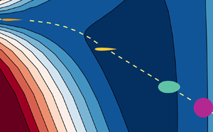
Figure 5. Contour plots of the Appellian vs the shape-control parameter  $D$ and the circulation (normalized by Kutta's). The yellow curve presents the locus of the minimizing circulation $\varGamma ^{\star }$. For $D=0$ (i.e. a sharp-edged airfoil), the minimizing circulation $\varGamma ^*$ coincides with Kutta's $\varGamma _K$; and for $D=1$ (circular cylinder), the minimizing circulation vanishes, implying no inviscid lifting capability of this purely symmetric shape. That is, the developed theory could capture the spectrum between the two extremes: from a zero lift over a circular cylinder to the Kutta–Zhukovsky lift over a sharp-edged airfoil. And the fact that the Kutta condition is a special case of the developed inviscid theory challenges the accepted wisdom about the viscous nature of the Kutta condition. It is not a manifestation of viscous effects, but rather momentum conservation.
It is important to note that the proposed variational theory is not confined to the steady flow past an airfoil with the free parameter being the bound circulation. In fact, the theorem provided in Appendix A rigorously establishes the connection/equivalence between minimization of the Appellian and Euler's partial differential equation with its vast generality, governing the dynamics of three-dimensional unsteady, but inviscid, flow fields. So, the current formulation is expected to be suitable for many other problems (e.g. Föppl Reference Föppl1983) where the flow field is parameterized in a more complicated way than just a single parameter (e.g. vortex patches). Then, minimizing the Appellian with respect to the free (undetermined) parameters in the model will provide equations governing the dynamics of these parameters; i.e. it will provide a rigorous way of projecting Euler's equation on the manifold of these parameters.
For example, the current formulation can be extended to determine the individual circulations over an array of airfoils. Crowdy (Reference Crowdy2006) developed an analytical solution for the flow field over a finite stack of airfoils using his prime function approach (Crowdy Reference Crowdy2020) when the strength of the bound circulation over each airfoil is known. So, the current formulation can be used complementarily with his effort to write the Appellian as a function of these circulations; i.e.  $S=S(\varGamma _0,\ldots \varGamma _M)$, where $M+1$ is the number of airfoils. Then, minimization of the Appellian with respect to the $M+1$ parameters will yield the dynamically correct circulations and flow field. Adding free vortices in the wake (Bai, Li & Wu Reference Bai, Li and Wu2014) should also be straightforward.
6. Discussion
The last section presents a new theory of lift based on Hertz’ variational principle of least curvature. In particular, (5.3) presents the sought general fundamental principle that provides closure in potential flow based on first principles (Hertz’ principle of least curvature), thereby generalizing the century-old theory of Kutta and Zhukovsky. This principle allows, for the first time, computation of lift over smooth shapes without sharp edges where the Kutta condition fails, which confirms that a sharp trailing edge is not a necessary condition for lift generation (Stack & Lindsey Reference Stack and Lindsey1938; Herrig, Emery & Erwin Reference Herrig, Emery and Erwin1956). The new variational theory, unlike the classical one, is capable of capturing the whole spectrum between the two extremes: from zero lift over a circular cylinder to the Kutta–Zhukovsky lift over an airfoil with a sharp trailing edge, as shown in figure 5(d). This behaviour provides credibility to the developed theory.
The fact that the minimization principle (5.3) reduces to the Kutta condition in the special case of a sharp-edged airfoil, wedded to the fact that this principle is an inviscid principle imply that the classical Kutta–Zhukovky lift over an airfoil with a sharp edge is both computed and explained from inviscid considerations. This finding challenges the accepted wisdom about the Kutta condition being a manifestation of viscous effects. Rather, it represents inviscid momentum conservation. That is, the circulation (and lift) is the one that satisfies momentum conservation – equivalently, it is the one that minimizes the Appellian in the language of Hertz. This result explains the several inviscid computations that converged to the Kutta–Zhukovky lift without viscosity (Rizzi Reference Rizzi1982; Yoshihara et al. Reference Yoshihara, Norstrud, Boerstoel, Chiocchia and Jones1985; Hoffman et al. Reference Hoffman, Jansson and Johnson2016; Musser et al. Reference Musser, Proment, Onorato and Irvine2019).
It should be noted that the prevalent attribution and association between viscosity and the origins of lift and the Kutta condition have not been gratuitous. A high-Reynolds-number flow over an airfoil at a small angle of attack is a singular perturbation problem where the small parameter is multiplying the highest derivative term (i.e. the viscous term; see Nayfeh Reference Nayfeh1973). Indeed, if this term is retained and the no-slip boundary condition is applied, there will be no ambiguity or a closure problem; the viscous solution will capture the right amount of lift and circulation. It is only when we neglect such a viscous term and ignore the no-slip boundary condition that a closure problem emerges. This singular behaviour is misleading and has shaped the common understanding of the viscous origin of lift and Kutta condition over the years. To dissect the physics of this problem, we simply need to remove viscosity altogether and solve the purely inviscid flow dynamics without any ad-hoc closure conditions (e.g. the Kutta condition) that may contaminate the inviscid nature of the solution; permitting a solution which emerges solely from physical principles. This is precisely what is enabled by the developed theory, which results in an inviscid lifting capability, driven by a necessary condition of momentum conservation.
We emphasize that the current result does not imply no role of viscosity in the picture. Rather, we argue that vorticity is a reaction, not the action; it is not the cause for circulation development. The vorticity in the boundary layer is a reaction to the outer inviscid flow. The main role of the boundary layer is to match the surface tangential velocity (for no slip) with the outer inviscid edge velocity; the latter is dictated by the inviscid fluid dynamics. This concept is not any different from Prandtl's classical formulation (Prandtl Reference Prandtl1904). However, the new contribution here asserts that the inviscid fluid dynamics is sufficient to determine the outer inviscid flow field (ignoring the secondary effects of interaction between the outer and inner solutions through modifying the effective shape of the body: body plus boundary layer). That is, the inviscid fluid dynamics is sufficient (and actually necessary too) to determine lift and circulation over the airfoil. In other words, in the current formulation, the integral of vorticity in the boundary layer would still sum up to the circulation around the airfoil, but the latter is dictated by inviscid fluid dynamics, and the former is developed as a reaction to this inviscid mechanism. Note that for a purely inviscid two-dimensional flow, the circulation around an irreducible circuit in a doubly connected domain is not the integral of vorticity over the area enclosed by the circuit (Karamcheti Reference Karamcheti1966).
The developed theory and obtained results are intimately related to the ability of an ideal fluid (superfluid) to generate lift. So, it may be prudent to discuss the seeming contradiction between Craig and Pellam's experimental result (Craig & Pellam Reference Craig and Pellam1957) and the recent computations by Musser et al. (Reference Musser, Proment, Onorato and Irvine2019), in the light of the developed theory. Craig and Pellam have experimentally studied the flow of an ideal fluid (superfluid helium II) over a flat plate and an ellipse and found a vanishingly small lift force over these objects at non-zero angles of attack. Hence, they concluded that superfluids are non-lifting and that ‘the classical viscosity boundary condition at the trailing edge (the Kutta condition) does not apply’ (Craig Reference Craig1959) – the last part of this statement about the viscous nature of the Kutta condition is refuted above.
Note that it is already known that the smaller the viscosity (i.e. the larger the Reynolds number), the larger the lift. So, as viscosity is decreased, lift either increases or remains constant. That is, the lift value in the limit to a vanishingly small viscosity is finite: the Kutta–Zhukovsky lift. Therefore, the above question about the non-lifting nature of superfluids is interesting from a physics perspective because if the hypothesis were true, it would represent one example in nature where the physics is not continuous in the limit; the limit of lift as viscosity approaches zero is different from the lift value at strictly zero viscosity (i.e. inviscid).
In contrast to the above hypothesis, Musser et al. (Reference Musser, Proment, Onorato and Irvine2019) recently performed quantum simulations of the Gross–Pitaevskii equation governing the flow dynamics over an airfoil in a superfluid. Their simulations show a quantized version of the Kutta–Zhukovsky lift despite the lack of viscosity in their simulations. However, the continuum hypothesis may not be applicable in their ultra-small-scale simulations.
From the above discussion, there seems to be a contradiction between Craig and Pellam's experiment (Craig & Pellam Reference Craig and Pellam1957) and the computations of Musser et al. (Reference Musser, Proment, Onorato and Irvine2019): the former may be misleading, implying that superfluids are non-lifting and the Kutta condition is a viscous condition (i.e. the physics is discontinuous in the limit), while the latter shows the ability of a superfluid to generate the Kutta–Zhukovsky lift similar to a viscous flow of a vanishingly small viscosity (i.e. the physics is continuous in the limit). In the light of the developed theory, we find no contradiction between the two results. In fact, Craig and Pellam conducted their experiment on symmetric shapes (a flat plate and an ellipse) for which the current theory predicts no lift, which confirms their experimental findings (but not their conclusions). Also, the current theory predicts Kutta–Zhukovsky lift over an airfoil with a sharp trailing edge; and a smaller but non-zero lift over a smooth airfoil (or asymmetric shape), which confirms Musser et al. (Reference Musser, Proment, Onorato and Irvine2019) computational simulations. Therefore, it is concluded that a purely symmetric (for-aft and top-bottom) shape in a superfluid is non-lifting; however, any asymmetry would grant some lifting capability. The current theory, as well as Musser et al. (Reference Musser, Proment, Onorato and Irvine2019) quantum simulations, invoke an experimental study of the flow of a superfluid (helium II), similar to Craig and Pellam's (Craig & Pellam Reference Craig and Pellam1957), but over a traditional airfoil shape (i.e. asymmetric shape). It is perhaps noteworthy to mention that superfluids are not exactly ideal fluids; however, from a continuum fluid mechanics perspective, they can be made to behave like ideal fluids, as demonstrated in Craig and Pellam's experiment.
The fact that purely symmetric shapes are non-lifting in an ideal (non-dissipative) fluid is physically plausible, as shown in figure 6(a) presenting the flow of an ideal fluid over a flat plate as predicted by the current theory. These flows must be reversible to conserve entropy in the dissipation-free environment. Therefore, for reversibility and because of symmetry, one should not be able to tell whether the flow field, shown in figure 6(a), is for a free stream coming from the left at a positive  $\alpha$ or from the right at a negative $\alpha$. Clearly, this symmetric solution is non-lifting.

Figure 6. Flow velocity,  $u/U$, of a superfluid (using the current theory) and a real fluid (using DES) over a flat plate at $\alpha =2^\circ$. Black and yellow lines are streamlines. (a) Current theory, (b) real fluid (DES computation).
For these symmetric shapes, viscosity is important to enable the weak lift over these bodies: the slight change of the effective body shape due to boundary layer destroys symmetry; the outer inviscid flow over the modified asymmetric body is now lifting. The flat plate represents an extreme case in this regard: the effect of viscosity is significant due to the singular nature of the corresponding ideal flow field. Viscosity leads to separation at the leading edge even at small angles of attack, as shown in the zoomed picture in figure 6(b), which presents our detached eddy simulation (DES) of the flow over a flat plate at a Reynolds number of 500 000 and  $\alpha =2^\circ$ (also see Van Dyke's album of fluid motion Van Dyke Reference Van Dyke1982 for a similar picture at $\alpha =2.5^\circ$). A leading-edge separation bubble is clearly seen on the top of the flat plate in the immediate vicinity of the leading edge. The outer inviscid flow field outside the separation bubble (i.e. over the modified flat plate: a flat plate with a naturally rounded nose) is lifting; the minimization principle (5.3), which is equivalent to the Kutta condition in this case of a sharp trailing edge, results in a circulation $\varGamma ^{\star }$ that is close to Kutta's. For a more detailed presentation on this topic, the reader is referred to the recent effort by Taha & Gonzalez (Reference Taha and Gonzalez2022a).
The developed theory is expected to deepen our understanding of one of the most fundamental concepts in aerodynamics: lift generation over an airfoil. It should open the doors for theoretical modelling of aerodynamics, as the developed variational principle, unlike the Kutta condition, is derived from first principles, allowing extensions of the aerodynamic theory to more challenging problems. In fact, we should emphasize that the variational principle (4.7) is also valid for unsteady problems; the unsteady term  ${\partial \boldsymbol {u}}/{\partial t}$ will have to be accounted for in the acceleration $\boldsymbol {a}$, which will be tackled in the future to determine the unsteady evolution of circulation (and lift) dynamics; i.e. the Wagner's problem (Wagner Reference Wagner1925; Chow & Huang Reference Chow and Huang1982; Graham Reference Graham1983; Li & Wu Reference Li and Wu2015). In this case, the rate of change of circulation ${{\rm d}\varGamma }/{{\rm d} t}$ will be the free parameter at each instant that is obtained by minimizing the instantaneous unsteady Appellian.
Finally, it may be prudent to provide a simple explanation for lift generation in the light of the obtained results and presented discussion – an explanation that does not invoke complex unsteady phenomena to illustrate how/why a particular steady lift value is attained. It is found that lift can be computed and explained using the triplet (4.7), (4.8), (4.9). In words, lift is due to (i) momentum conservation, (ii) continuity (the fluid has to fill the given space), and (iii) the body's hard constraint (i.e. presence of the body inside the fluid), which forces the flow to move around the body without creating void to maintain (ii). That is, lift is due to conservation of momentum between the two equilibrium states of the free stream and the curved flow around the body. In layman terms, the presence of the body inside the fluid forces fluid particles to go along a curved path; i.e. it provides the necessary centripetal force for the curved path. And the fluid responds back by an equal amount of force in the opposite direction according to Newton's third law – this reaction is the lift force. This explanation is similar to Hoffren's (Hoffren Reference Hoffren2000) and to some extent to Babinsky's (Babinsky Reference Babinsky2003); the current paper provides the sought mathematical framework. Inventors and analysts alike may find it intriguing that a dry water model (Feynman Reference Feynman1964) provides the main physical mechanism behind one of most fundamental problems in fluid mechanics.
7. Conclusion
We revived the deserted variational principle of least curvature by Hertz’ to develop a novel variational principle for the dynamics of ideal fluids. The developed variational principle is fundamentally different from the previous variational formulations based on Hamilton's principle of least action. It provides unique solutions in some of the singular cases where Lagrangian (and Newtonian) mechanics fail. In particular, it provides a unique solution for the circulation over an airfoil where Euler's equation requires a closure condition to determine the value of circulation – aka the Kutta condition. That is, the developed variational principle provides a general dynamical closure condition for the airfoil problem that is, unlike the Kutta condition, derived from first principles: Hertz’ principle of least curvature. As such, the developed variational principle is not confined to sharp-edged airfoils, in contrast to the classical theory. That is, it allows, for the first time, computation of lift over smooth cylindrical shapes (without sharp edges). The (inviscid) variational principle reduces to the Kutta condition in the special case of a sharp-edge airfoil, which challenges the accepted wisdom about the Kutta condition being a manifestation of viscous effects; it has long been thought that the Kutta condition implicitly accounts for viscous effects within the potential-flow formulation. In contrast, it is found to be a condition for momentum conservation in ideal fluids. This conclusion sheds some light on the ability of a superfluid to generate lift. The developed variational principle provides conditions on the geometry of a given shape to generate lift in an inviscid fluid. The shape must have some fore-aft asymmetry to generate an increasing lift with the angle of attack. That is, a purely symmetric shape (e.g. flat plate, ellipse, circular cylinder) is non-lifting in a purely inviscid medium. In reality, viscosity is essential to enable the weak lift over these shapes with the flat plate being a special case where viscosity plays a significant role; it triggers separation at the leading edge (even at small angles of attack), which destroys the symmetry, enabling the Kutta–Zhukovsky lift.
Acknowledgements
The authors are grateful for the many fruitful discussions with Profs S. Ragab, J. Loviscach, N. Nguyen, P. Baddoo, K. McKee, W. Sirignano, T. Georgiou, M. Zakaria and Y. Aboelkassem.
Funding
This work was partially supported by the National Aeronautics and Space Administration Fellowship 80NSSC20K1474 that supported the PhD of C. G. Otherwise, this research received no specific grant from any funding agency, commercial or not-for-profit sectors.
Declaration of interests
The authors report no conflict of interest.
Author contributions
H.T. introduced the use of variational principles in the airfoil problem; C.G. hypothesized the minimality of curvature and total acceleration; developed the analytical framework to determine circulation on arbitrary cylinders, recovering Kutta's result. H.T. drew the connection with Gauss’ principle; C.G. reduced it to Hertz’ principle and conjectured the constraint nature of the pressure force; H.T. proved it; C.G. proved non-lifting properties of the circular cylinder and showed that lift requires asymmetry in the conformal mapping. H.T. provided the variational formulation of Euler's equation and proved the equivalence theorem; C.G. performed numerical simulations of the theory and computational fluid dynamics simulations; C.G. also studied convergence and created the figures; H.T. wrote the draft of the paper; and both authors finalized the manuscript.
Appendix A. Equivalence between Euler's equation and minimization of the Appellian for incompressible flows
Theorem If  $\boldsymbol {u}_t(\boldsymbol {x})\equiv {\partial \boldsymbol {u}}/{\partial t}$ is continuously differentiable in $\varOmega \subset \mathbb {R}^3$ and minimizes the functional
 \begin{equation} S(\boldsymbol{u}_t(\boldsymbol{x})) = \frac{1}{2}\int_\varOmega \rho \left(\boldsymbol{u}_t(\boldsymbol{x})+\boldsymbol{u}(\boldsymbol{x})\boldsymbol{\cdot}\boldsymbol{\nabla} \boldsymbol{u}(\boldsymbol{x})\right)^2 {\rm d}\kern0.06em \boldsymbol{x} \end{equation}
for all  $t\in \mathbb {R}$ subject to the constraint
 \begin{equation} \boldsymbol{\nabla} \boldsymbol{\cdot}\boldsymbol{u}=0 \quad \forall\ \boldsymbol{x}\in\varOmega, \enspace t\in\mathbb{R}, \end{equation}
and the no-penetration boundary condition
 \begin{equation} \boldsymbol{u}\boldsymbol{\cdot} \boldsymbol{n} = 0,\quad \forall \boldsymbol{x}\in\partial\varOmega, \enspace t\in\mathbb{R}, \end{equation}
where  $\boldsymbol {n}$ is normal to the boundary $\partial \varOmega$, then $\boldsymbol {u}_t(\boldsymbol {x})$ must satisfy
 \begin{equation} \rho\left(\boldsymbol{u}_t+\boldsymbol{u}\boldsymbol{\cdot}\boldsymbol{\nabla} \boldsymbol{u}\right)={-}\boldsymbol{\nabla} p \quad \forall\ \boldsymbol{x}\in\varOmega,\enspace t\in\mathbb{R} \end{equation}
for some differentiable function  $p$ on $\varOmega$.
Proof. If the constraint  $\boldsymbol {\nabla } \boldsymbol {\cdot }\boldsymbol {u}=0$ must be satisfied for all $t$, then it implies that $\boldsymbol {\nabla } \boldsymbol {\cdot }\boldsymbol {u}_t=0$. Then, to minimize $S$ subject to the constraint $\boldsymbol {\nabla } \boldsymbol {\cdot }\boldsymbol {u}_t=0$ for all $\boldsymbol {x}\in \varOmega$, we construct the Lagrangian
 \begin{equation} \mathcal{L} = S - \int_\varOmega p(\boldsymbol{x}) \left(\boldsymbol{\nabla} \boldsymbol{\cdot}\boldsymbol{u}_t(\boldsymbol{x})\right) {\rm d}\kern0.06em \boldsymbol{x}, \end{equation}
where  $p$ is a Lagrange multiplier. A necessary condition for the constrained minimization problem is then: the first variation of the Lagrangian vanishes with respect to variations in $\boldsymbol {u}_t(\boldsymbol {x})$. The first variation of $\mathcal {L}$ with respect to $\boldsymbol {u}_t$ is written as
 \begin{equation} \delta\mathcal{L} = \int_\varOmega [\rho \left(\boldsymbol{u}_t+\boldsymbol{u}\boldsymbol{\cdot}\boldsymbol{\nabla} \boldsymbol{u}\right) \boldsymbol{\cdot}\delta \boldsymbol{u}_t - p \boldsymbol{\nabla} \boldsymbol{\cdot}\delta\boldsymbol{u}_t] {\rm d}\kern0.06em \boldsymbol{x}=0. \end{equation}
The last term  $p \boldsymbol {\nabla } \boldsymbol {\cdot }\delta \boldsymbol {u}_t$ can be written as
 \begin{equation} p \boldsymbol{\nabla} \boldsymbol{\cdot}\delta\boldsymbol{u}_t = \boldsymbol{\nabla} \boldsymbol{\cdot} (p\delta\boldsymbol{u}_t)-\boldsymbol{\nabla} p \boldsymbol{\cdot} \delta\boldsymbol{u}_t. \end{equation}
Integrating the first component  $\boldsymbol {\nabla } \boldsymbol {\cdot } (p\delta \boldsymbol {u}_t)$ and using the divergence theorem, we have
 \begin{equation} \int_\varOmega \boldsymbol{\nabla} \boldsymbol{\cdot} (p\delta\boldsymbol{u}_t)\,{\rm d}\kern0.06em \boldsymbol{x} = \int_{\partial\varOmega} p\delta\boldsymbol{u}_t\boldsymbol{\cdot}\boldsymbol{n} \,{\rm d}\kern0.06em \boldsymbol{x}. \end{equation}
Since  $\boldsymbol {u}\boldsymbol {\cdot } \boldsymbol {n}$ is specified on the boundary for all $t$, it implies that $\boldsymbol {u}_t\boldsymbol {\cdot } \boldsymbol {n}$ is also specified on the boundary. As such, its variation $\delta \boldsymbol {u}_t\boldsymbol {\cdot } \boldsymbol {n}$ must vanish on the boundary, resulting in $\int _\varOmega \boldsymbol {\nabla } \boldsymbol {\cdot } (p\delta \boldsymbol {u}_t) d\boldsymbol {x}=0$. Hence, we have
 \begin{equation} \delta\mathcal{L} = \int_\varOmega [\rho \left(\boldsymbol{u}_t+\boldsymbol{u}\boldsymbol{\cdot}\boldsymbol{\nabla} \boldsymbol{u}\right) + \boldsymbol{\nabla} p]\cdot \delta \boldsymbol{u}_t \,{\rm d}\kern0.06em \boldsymbol{x}=0 \end{equation}
for all admissible variations  $\delta \boldsymbol {u}_t$, which implies that
 \begin{equation} \rho\left(\boldsymbol{u}_t+\boldsymbol{u}\boldsymbol{\cdot}\boldsymbol{\nabla} \boldsymbol{u}\right)={-}\boldsymbol{\nabla} p \quad \forall \boldsymbol{x}\in\varOmega,\enspace t\in\mathbb{R}. \end{equation}
The above theorem is a special case of the theorem provided by Taha & Gonzalez (Reference Taha and Gonzalez2022b) where they generalized the current formulation to viscous fluids governed by Navier–Stokes’ equation.
The above theorem shows that a solution that minimizes the Appellian automatically satisfies Euler's equation. However, we conjecture that the converse may not be true. While an Euler's solution extremizes the Appellian, we conjecture that only the stable solutions of Euler's equation are minimizing the Appellian, and the unstable ones are maximizers instead. This variational formulation of hydrodynamic stability, which is inspired by Arnold's work (Arnold Reference Arnold1966), will be pursued in the future.


 Open access