


1 Introduction
Isothermal non-coalescence phenomena between a droplet and a wall or a liquid surface can occur under various conditions. Examples include droplet levitation over moving solid walls (Neitzel et al. Reference Neitzel, Dell’Aversana, Tontodonato, Vetrano, Minster and Schürmann2001; Smith & Neitzel Reference Smith and Neitzel2006; Lhuissier et al. Reference Lhuissier, Tagawa, Tran and Sun2013; Saito & Tagawa Reference Saito and Tagawa2015; Gauthier et al. Reference Gauthier, Bird, Clanet and Quéré2016), atomically smooth horizontal walls (de Ruiter et al. Reference de Ruiter, Lagraauw, Mugele and van den Ende2015), inclined walls (Hodges, Jensen & Rallison Reference Hodges, Jensen and Rallison2004; Gilet & Bush Reference Gilet and Bush2012; Harris, Liu & Bush Reference Harris, Liu and Bush2015) and vibrating/moving liquid surfaces (Sreenivas, De & Arakeri Reference Sreenivas, De and Arakeri1999; Couder et al. Reference Couder, Fort, Gautier and Boudaoud2005; Terwagne, Vandewalle & Dorbolo Reference Terwagne, Vandewalle and Dorbolo2007; Gilet et al. Reference Gilet, Terwagne, Vandewalle and Dorbolo2008; Che, Deygas & Matar Reference Che, Deygas and Matar2015). The isothermal non-coalescence phenomena can be explained as follows. Lubrication pressure is generated inside an air film of several micrometres in thickness between the droplet and the wall. When the lubrication force (the area integral of the lubrication pressure) overcomes the gravitational force acting on the droplet, the non-coalescence phenomena can occur. The lubrication pressure depends on the shape of the air film (Neitzel & Dell’Aversana Reference Neitzel and Dell’Aversana2002). The film shape, including the free surface of the droplet, is determined by the local balance of the lubrication pressure and the surface tension and hydrostatic pressures (Lhuissier et al. Reference Lhuissier, Tagawa, Tran and Sun2013). However, to the best of the authors’ knowledge, such balances have not been experimentally verified for a wide range of parameters. Furthermore, previous research has not paid much attention to the effect of droplet viscosity on the ‘steady’ air film shape under levitating droplets. To avoid confusion in this paper, we use ‘stable’ and ‘steady’ for the state of droplet levitation and the state of the air film, respectively.
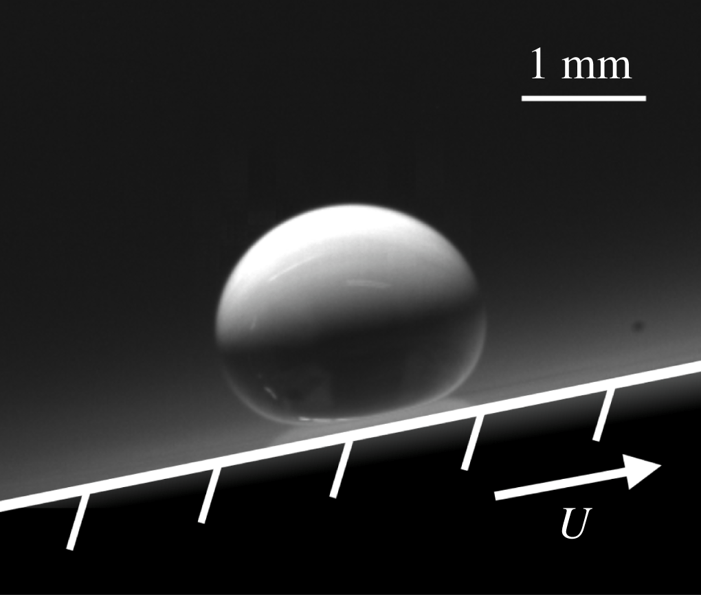
Figure 1. Side view of a levitating droplet over a moving wall. $U$
is the wall’s velocity.
$U$
is the wall’s velocity.
We briefly summarize previous studies of non-coalescence phenomena between droplets and a moving wall or liquid surface closely related to our study. Neitzel et al. (Reference Neitzel, Dell’Aversana, Tontodonato, Vetrano, Minster and Schürmann2001) investigated non-coalescence phenomena between a rotating disk and a droplet attached to a fixed support. They confirmed a steady shape of the air film between the fixed droplet and the rotating disk. For this situation, Smith & Neitzel (Reference Smith and Neitzel2006) computed the pressure distribution generated inside the air film by two-dimensional numerical simulations. Gauthier et al. (Reference Gauthier, Bird, Clanet and Quéré2016) deposited a droplet onto a rotating disk, resulting in unstable behaviour of the droplet. Lhuissier et al. (Reference Lhuissier, Tagawa, Tran and Sun2013) levitated a droplet over an inner wall of a rotating glass cylinder. They numerically computed the two-dimensional film shape by considering the local balance of the lubrication pressure and the surface tension and hydrostatic pressures at the bottom of the droplet. The computed shape qualitatively agreed with the measured shape. Sreenivas et al. (Reference Sreenivas, De and Arakeri1999) estimated the thickness of the air film for droplets levitating over a moving liquid surface near a hydraulic jump by considering the force balance of the droplets. They also estimated the surface velocity of the droplet for a rotating motion caused by viscous shear exerted on the bottom of the droplet. However, their estimations have not been experimentally verified for a wide range of parameters.
In this paper, we focus on a levitating droplet over a moving wall that is in our case a rotating glass cylinder, as shown in figure 1 and movie 1 available at https://doi.org/10.1017/jfm.2018.952. Both the steady air film shape and the stable droplet behaviour should help us examine the levitating droplet experimentally in detail. First, we investigate the effects of droplet viscosity on the surface velocity of a levitating droplet and the steady state of the air film shape (§ 4). Next, we verify two kinds of force/pressure balances for a steady-shape air film (§ 5). One is the force balance acting on the levitating droplet. The lift force should balance with the drag and gravity forces. We compute the lift force generated inside the air film by integrating the lubrication pressure. The other is the local pressure balance at the bottom of the droplet. We calculate the surface tension and hydrostatic pressures from the measured air film in our experiment. Notably, the results present a good agreement between the two kinds of force/pressure balances. Finally, we discuss how the shape of the air film is determined.

Figure 2. Coordinate system and parameters for a levitating droplet.
2 Theory
2.1 Lubrication theory
In our experiments, the air film thickness (several micrometres) is sufficiently small compared to the characteristic length along the mainstream of the air flow, namely the droplet diameter $d$
(a few millimetres; see figure 2). Therefore, we can apply lubrication theory to the air film (Saito & Tagawa Reference Saito and Tagawa2015). A detailed verification is shown in appendix A. Figure 2 shows a coordinate system and parameters for a levitating droplet over a moving wall where the centroidal position projected onto the wall is set as the origin of the coordinate system. The
$d$
(a few millimetres; see figure 2). Therefore, we can apply lubrication theory to the air film (Saito & Tagawa Reference Saito and Tagawa2015). A detailed verification is shown in appendix A. Figure 2 shows a coordinate system and parameters for a levitating droplet over a moving wall where the centroidal position projected onto the wall is set as the origin of the coordinate system. The $x$
-,
$x$
-, $y$
- and
$y$
- and $z$
-axes represent, respectively, the direction of wall motion, the direction normal to the
$z$
-axes represent, respectively, the direction of wall motion, the direction normal to the $x$
-axis on the wall and the direction normal to the wall. The air film thickness is
$x$
-axis on the wall and the direction normal to the wall. The air film thickness is $h(x,y)$
. In order to determine the equation of motion for the air film with constant wall velocity
$h(x,y)$
. In order to determine the equation of motion for the air film with constant wall velocity $U$
, we assume the following conditions: (i) an incompressible and Newtonian fluid, (ii) a constant dynamic viscosity of the air, (iii) laminar flow, (iv) negligible gravity and inertia forces, (v) constant pressure in the
$U$
, we assume the following conditions: (i) an incompressible and Newtonian fluid, (ii) a constant dynamic viscosity of the air, (iii) laminar flow, (iv) negligible gravity and inertia forces, (v) constant pressure in the $z$
-direction and (vi) no-slip condition on the droplet surface. Note that Reynolds number
$z$
-direction and (vi) no-slip condition on the droplet surface. Note that Reynolds number $Re=\unicode[STIX]{x1D70C}Uh^{2}/\unicode[STIX]{x1D707}d$
which considers a geometrical aspect ratio is
$Re=\unicode[STIX]{x1D70C}Uh^{2}/\unicode[STIX]{x1D707}d$
which considers a geometrical aspect ratio is $O(10^{-4})$
; in other words,
$O(10^{-4})$
; in other words, $Re$
is sufficiently smaller than unity (see appendix A). Parameters
$Re$
is sufficiently smaller than unity (see appendix A). Parameters $\unicode[STIX]{x1D70C}$
and
$\unicode[STIX]{x1D70C}$
and $\unicode[STIX]{x1D707}$
indicate the density of the air and the dynamic viscosity of the air, respectively. Moreover, we assume that the surface velocity of the droplet
$\unicode[STIX]{x1D707}$
indicate the density of the air and the dynamic viscosity of the air, respectively. Moreover, we assume that the surface velocity of the droplet $u$
is negligible since it is in the range of
$u$
is negligible since it is in the range of $2.5\times 10^{-3}{-}2.4\times 10^{-1}~\text{m}~\text{s}^{-1}$
, much smaller than the wall velocity
$2.5\times 10^{-3}{-}2.4\times 10^{-1}~\text{m}~\text{s}^{-1}$
, much smaller than the wall velocity $U$
(of the order of
$U$
(of the order of $1~\text{m}~\text{s}^{-1}$
; see § 4). The above assumptions give an equation of motion in the air film as (Tipei Reference Tipei1962; Saito & Tagawa Reference Saito and Tagawa2015)
$1~\text{m}~\text{s}^{-1}$
; see § 4). The above assumptions give an equation of motion in the air film as (Tipei Reference Tipei1962; Saito & Tagawa Reference Saito and Tagawa2015)
 $$\begin{eqnarray}\frac{\unicode[STIX]{x2202}}{\unicode[STIX]{x2202}x}\left(\frac{h^{3}}{\unicode[STIX]{x1D707}}\frac{\unicode[STIX]{x2202}p}{\unicode[STIX]{x2202}x}\right)+\frac{\unicode[STIX]{x2202}}{\unicode[STIX]{x2202}y}\left(\frac{h^{3}}{\unicode[STIX]{x1D707}}\frac{\unicode[STIX]{x2202}p}{\unicode[STIX]{x2202}y}\right)=6U\frac{\unicode[STIX]{x2202}h}{\unicode[STIX]{x2202}x},\end{eqnarray}$$
where $p(x,y)$
is the lubrication pressure generated inside the air film and
$p(x,y)$
is the lubrication pressure generated inside the air film and $\unicode[STIX]{x1D707}$
is the dynamic viscosity of the air. We can calculate
$\unicode[STIX]{x1D707}$
is the dynamic viscosity of the air. We can calculate $p(x,y)$
using (2.1) if
$p(x,y)$
using (2.1) if $h(x,y)$
is known. Based on the analysis of propagation of errors from the experimental parameters
$h(x,y)$
is known. Based on the analysis of propagation of errors from the experimental parameters $h$
,
$h$
, $U$
and
$U$
and $\unicode[STIX]{x1D707}$
on the lubrication pressure
$\unicode[STIX]{x1D707}$
on the lubrication pressure $p$
, we find that the error of the air film thickness
$p$
, we find that the error of the air film thickness $h$
is dominant in comparison with the other parameters (see appendix B). We define a thin-film area of diameter
$h$
is dominant in comparison with the other parameters (see appendix B). We define a thin-film area of diameter $d_{t}$
as the area where the lubrication pressure
$d_{t}$
as the area where the lubrication pressure $p$
is generated (see appendix C). As a boundary condition, the rim of the thin-film area is taken to be at atmospheric pressure (
$p$
is generated (see appendix C). As a boundary condition, the rim of the thin-film area is taken to be at atmospheric pressure ( $p=0$
in gauge). We solve (2.1) by the finite difference method using MATLAB for repeating calculations.
$p=0$
in gauge). We solve (2.1) by the finite difference method using MATLAB for repeating calculations.
2.2 Force/pressure balances
We experimentally verify the force/pressure balances acting on the droplet. First we compare the lift force $L$
and the droplet’s weight
$L$
and the droplet’s weight $W$
. We call this balance the ‘global balance’. Lift force
$W$
. We call this balance the ‘global balance’. Lift force $L$
in the direction normal to the wall is calculated as
$L$
in the direction normal to the wall is calculated as
 $$\begin{eqnarray}L=\iint p\,\text{d}x\,\text{d}y.\end{eqnarray}$$
The integration range of (2.2) is the thin-film area (see appendix C). Note that a measurement error of $h$
results in a measurement error in
$h$
results in a measurement error in $L$
, because the error of the air film thickness
$L$
, because the error of the air film thickness $h$
is dominant on lubrication pressure
$h$
is dominant on lubrication pressure $p$
as mentioned above. In our experiments, the maximum measurement error of
$p$
as mentioned above. In our experiments, the maximum measurement error of $L$
is 11 %.
$L$
is 11 %.
Convergence condition on repeating calculations of the lift $L$
is defined as the case in which the difference between the lift
$L$
is defined as the case in which the difference between the lift $L$
at the
$L$
at the $k$
th calculation and the lift
$k$
th calculation and the lift $L$
at the
$L$
at the $(k-10\,000)$
th calculation is less than or equal to
$(k-10\,000)$
th calculation is less than or equal to $1\times 10^{-3}\,\%$
. The thin-film area is divided in
$1\times 10^{-3}\,\%$
. The thin-film area is divided in $500\times 500$
for the calculations of the lubrication pressure
$500\times 500$
for the calculations of the lubrication pressure $p$
and the lift
$p$
and the lift $L$
. The difference between the lift
$L$
. The difference between the lift $L$
for the
$L$
for the $500\times 500$
case and that for the
$500\times 500$
case and that for the $1000\times 1000$
case is less than 0.3 %. The droplet rests at a point where the lift force balances with the drag and gravity forces in a glass cylinder with constant rotating velocity. Weight
$1000\times 1000$
case is less than 0.3 %. The droplet rests at a point where the lift force balances with the drag and gravity forces in a glass cylinder with constant rotating velocity. Weight $W$
in the direction normal to the wall is expressed by
$W$
in the direction normal to the wall is expressed by
 $$\begin{eqnarray}W=mg\cos \unicode[STIX]{x1D703},\end{eqnarray}$$
where $m$
,
$m$
, $g$
and
$g$
and $\unicode[STIX]{x1D703}$
are the mass of the droplet, gravitational acceleration and the inclination angle of the droplet against the gravitational acceleration direction (see figure 3), respectively. The mass
$\unicode[STIX]{x1D703}$
are the mass of the droplet, gravitational acceleration and the inclination angle of the droplet against the gravitational acceleration direction (see figure 3), respectively. The mass $m$
is calculated based on the droplet diameter
$m$
is calculated based on the droplet diameter $d$
(detailed calculation is explained in § 3). The orders of magnitude for the errors of
$d$
(detailed calculation is explained in § 3). The orders of magnitude for the errors of $d$
and
$d$
and $m$
are 0.9 % and 2 %, respectively. The inclination angle
$m$
are 0.9 % and 2 %, respectively. The inclination angle $\unicode[STIX]{x1D703}$
is calculated from an arc length of the cylinder wall from the position on the cylinder wall at
$\unicode[STIX]{x1D703}$
is calculated from an arc length of the cylinder wall from the position on the cylinder wall at $\unicode[STIX]{x1D703}=0^{\circ }$
to the position at which the droplet levitates (see figure 3). We observe marks of two positions on the wall of the rotating cylinder by using a camera, and compute the arc length between two positions. The order of magnitude for the error of
$\unicode[STIX]{x1D703}=0^{\circ }$
to the position at which the droplet levitates (see figure 3). We observe marks of two positions on the wall of the rotating cylinder by using a camera, and compute the arc length between two positions. The order of magnitude for the error of $\unicode[STIX]{x1D703}$
is 6 %. Therefore, the error of the the weight
$\unicode[STIX]{x1D703}$
is 6 %. Therefore, the error of the the weight $W$
comes from the error of
$W$
comes from the error of $m$
and
$m$
and $\unicode[STIX]{x1D703}$
. In our experiments, the maximum measurement error of
$\unicode[STIX]{x1D703}$
. In our experiments, the maximum measurement error of $W$
is 2 %. When
$W$
is 2 %. When $L$
is quantitatively equal to
$L$
is quantitatively equal to $W$
, the global balance of the levitating droplet is satisfied.
$W$
, the global balance of the levitating droplet is satisfied.

Figure 3. Schematic view of the experimental set-up.
Next we verify the pressure balance at an arbitrary point on the bottom of the droplet. We call this balance the ‘local balance’. The lubrication pressure $p$
, surface tension and hydrostatic pressures are acting on the bottom of the levitating droplet (Lhuissier et al.
Reference Lhuissier, Tagawa, Tran and Sun2013). Without consideration of the air resistance and rotating motion inside the droplet, the local pressure balance is given as
$p$
, surface tension and hydrostatic pressures are acting on the bottom of the levitating droplet (Lhuissier et al.
Reference Lhuissier, Tagawa, Tran and Sun2013). Without consideration of the air resistance and rotating motion inside the droplet, the local pressure balance is given as
 $$\begin{eqnarray}2\unicode[STIX]{x1D70E}(\unicode[STIX]{x1D705}_{0}-\unicode[STIX]{x1D705})+\unicode[STIX]{x0394}\unicode[STIX]{x1D70C}g[(z_{0}-z)\cos \unicode[STIX]{x1D703}+(x_{0}-x)\sin \unicode[STIX]{x1D703}]=p,\end{eqnarray}$$
where the first and second terms on the left-hand side stand for the surface tension pressure and variation of hydrostatic pressure, respectively. Parameters $\unicode[STIX]{x1D70E}$
,
$\unicode[STIX]{x1D70E}$
, $\unicode[STIX]{x0394}\unicode[STIX]{x1D70C}$
,
$\unicode[STIX]{x0394}\unicode[STIX]{x1D70C}$
, $\unicode[STIX]{x1D705}$
and
$\unicode[STIX]{x1D705}$
and $\unicode[STIX]{x1D705}_{0}$
are the surface tension coefficient, density difference between the air and the liquid, mean curvature at the droplet’s interface and mean curvature at
$\unicode[STIX]{x1D705}_{0}$
are the surface tension coefficient, density difference between the air and the liquid, mean curvature at the droplet’s interface and mean curvature at $(x_{0},y_{0},z_{0})$
, respectively. The position
$(x_{0},y_{0},z_{0})$
, respectively. The position $(x_{0},y_{0},z_{0})$
is at the rim of the thin-film area, i.e.
$(x_{0},y_{0},z_{0})$
is at the rim of the thin-film area, i.e. $(x_{0}=-d_{t}/2,y_{0}=0,z_{0}=h(x_{0},y_{0})=H)$
. We define
$(x_{0}=-d_{t}/2,y_{0}=0,z_{0}=h(x_{0},y_{0})=H)$
. We define $p_{s}$
as the total pressure on the left-hand side of (2.4). We then compare
$p_{s}$
as the total pressure on the left-hand side of (2.4). We then compare $p$
and
$p$
and $p_{s}$
.
$p_{s}$
.
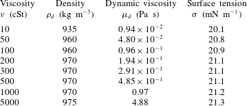
2.3 Surface velocity of a levitating droplet
The surface velocity of the levitating droplet $u$
can be calculated by a theoretical consideration:
$u$
can be calculated by a theoretical consideration:
 $$\begin{eqnarray}u\simeq \frac{U}{1+[2\overline{h}\unicode[STIX]{x1D707}_{d}/d^{\prime }\unicode[STIX]{x1D707}]},\end{eqnarray}$$
where $\overline{h}$
,
$\overline{h}$
, $\unicode[STIX]{x1D707}_{d}$
and
$\unicode[STIX]{x1D707}_{d}$
and $d^{\prime }$
are the average thickness of the air film, the dynamic viscosity of the droplet and droplet height, respectively. Here,
$d^{\prime }$
are the average thickness of the air film, the dynamic viscosity of the droplet and droplet height, respectively. Here, $\overline{h}$
in steady state depends on
$\overline{h}$
in steady state depends on $d^{\prime }$
and
$d^{\prime }$
and $U$
(we discuss it in detail in § 4). Therefore, equation (2.5) indicates that
$U$
(we discuss it in detail in § 4). Therefore, equation (2.5) indicates that $u$
depends only on
$u$
depends only on $\unicode[STIX]{x1D707}_{d}$
when
$\unicode[STIX]{x1D707}_{d}$
when $\unicode[STIX]{x1D707}$
,
$\unicode[STIX]{x1D707}$
, $d^{\prime }$
and
$d^{\prime }$
and $U$
are constant.
$U$
are constant.
3 Experiment
Figure 3 shows a schematic view of our experimental set-up (cf. Saito & Tagawa Reference Saito and Tagawa2015). A hollow silica-glass cylinder of 200 mm in diameter rotates on its axis with a constant wall velocity $U$
. A droplet of silicone oil is deposited onto the inner wall of the cylinder and levitates at a stable position where the forces acting on the droplet balance. Note that ‘stable’ is defined as the state in which variation of levitating angle
$U$
. A droplet of silicone oil is deposited onto the inner wall of the cylinder and levitates at a stable position where the forces acting on the droplet balance. Note that ‘stable’ is defined as the state in which variation of levitating angle $\unicode[STIX]{x1D703}$
is not greater than
$\unicode[STIX]{x1D703}$
is not greater than $2^{\circ }$
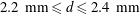
. We use several kinds of silicone oil for the droplet, the physical properties of which are shown in table 1.
$2^{\circ }$
. We use several kinds of silicone oil for the droplet, the physical properties of which are shown in table 1.
Table 1. Physical properties of silicone oil used for droplets.
In order to visualize flow motion inside a levitating droplet, tracer particles (diameter: $50~\unicode[STIX]{x03BC}\text{m}$
; specific gravity: 1.02) are mixed into the droplets. We trace a certain particle (PTV measurement) using a high-speed camera (FASTCAM SA-X, Photron Co.) at a shooting speed of 250 frames per second to measure the period of droplet rotation
$50~\unicode[STIX]{x03BC}\text{m}$
; specific gravity: 1.02) are mixed into the droplets. We trace a certain particle (PTV measurement) using a high-speed camera (FASTCAM SA-X, Photron Co.) at a shooting speed of 250 frames per second to measure the period of droplet rotation $T$
. To calculate the surface velocity
$T$
. To calculate the surface velocity $u$
, the following conditions are assumed: (I) the surface and inner velocities of the droplets are constant, (II) the droplets are under rigid-body rotation and (III) three-dimensional movement inside the droplet is negligible. The surface velocity
$u$
, the following conditions are assumed: (I) the surface and inner velocities of the droplets are constant, (II) the droplets are under rigid-body rotation and (III) three-dimensional movement inside the droplet is negligible. The surface velocity $u$
is then given as
$u$
is then given as
 $$\begin{eqnarray}u=\frac{C}{T},\end{eqnarray}$$
where $C$
indicates the circumference of the droplet. Circumference
$C$
indicates the circumference of the droplet. Circumference $C$
is calculated from the droplet diameter
$C$
is calculated from the droplet diameter $d$
by using Mathematica, assuming that the droplet is on a fixed wall for a contact angle of
$d$
by using Mathematica, assuming that the droplet is on a fixed wall for a contact angle of $180^{\circ }$
. This will be discussed in detail later in this section. The error on
$180^{\circ }$
. This will be discussed in detail later in this section. The error on $u$
is the standard error of the results of several numbers of particles tracked. Droplet diameter
$u$
is the standard error of the results of several numbers of particles tracked. Droplet diameter $d$
is changed in the range 2.0–2.4 mm and
$d$
is changed in the range 2.0–2.4 mm and $U$
is fixed at
$U$
is fixed at $1.57~\text{m}~\text{s}^{-1}$
. The viscosity of the silicone oil
$1.57~\text{m}~\text{s}^{-1}$
. The viscosity of the silicone oil $\unicode[STIX]{x1D708}$
ranges from 10 to 1000 cSt, that is, the dynamic viscosity
$\unicode[STIX]{x1D708}$
ranges from 10 to 1000 cSt, that is, the dynamic viscosity $\unicode[STIX]{x1D707}_{d}$
ranges from
$\unicode[STIX]{x1D707}_{d}$
ranges from $0.94\times 10^{-2}$
to 0.97 Pa s.
$0.94\times 10^{-2}$
to 0.97 Pa s.
The steady state of the air film is observed using an interferometric method. Monochromatic light of wavelength 630 nm illuminates the bottom of the droplet through a coaxial zoom lens ( $12\times$
Co-axial Ultra Zoom Lens, Navitar Co.). The reflected light from the bottom of the droplet and the wall forms interference fringes, namely, interference fringes are formed when the thickness of the air film
$12\times$
Co-axial Ultra Zoom Lens, Navitar Co.). The reflected light from the bottom of the droplet and the wall forms interference fringes, namely, interference fringes are formed when the thickness of the air film $h(x,y)$
is
$h(x,y)$
is $n/2$
of the wavelength of the incident light, where
$n/2$
of the wavelength of the incident light, where $n$
is an integer. We obtain an image of the fringes with a high-speed camera (FASTCAM SA-X, Photron Co.) at a shooting speed of 15 000 frames per second. We show a typical image of interference fringes in figure 4(a), where the arrow in the figure shows the direction of
$n$
is an integer. We obtain an image of the fringes with a high-speed camera (FASTCAM SA-X, Photron Co.) at a shooting speed of 15 000 frames per second. We show a typical image of interference fringes in figure 4(a), where the arrow in the figure shows the direction of $U$
. From the fringe pattern, we decide the state of the air film. We define a ‘steady state’ of the air film as the state in which variation of the minimum thickness of the air film is not greater than 630 nm (two fringes) over 0.05 s (see figure 5
a). In contrast, ‘unsteady state’ of the air film is defined as the state in which variation of the minimum thickness is greater than 630 nm (see figure 5
b). We change
$U$
. From the fringe pattern, we decide the state of the air film. We define a ‘steady state’ of the air film as the state in which variation of the minimum thickness of the air film is not greater than 630 nm (two fringes) over 0.05 s (see figure 5
a). In contrast, ‘unsteady state’ of the air film is defined as the state in which variation of the minimum thickness is greater than 630 nm (see figure 5
b). We change $\unicode[STIX]{x1D708}$
within 100–5000 cSt and
$\unicode[STIX]{x1D708}$
within 100–5000 cSt and $U$
within
$U$
within $0.59$
–
$0.59$
– $1.88~\text{m}~\text{s}^{-1}$
for droplet diameters in the range of
$1.88~\text{m}~\text{s}^{-1}$
for droplet diameters in the range of $2.2~\text{mm}\leqslant d\leqslant 2.4~\text{mm}$
.
$2.2~\text{mm}\leqslant d\leqslant 2.4~\text{mm}$
.
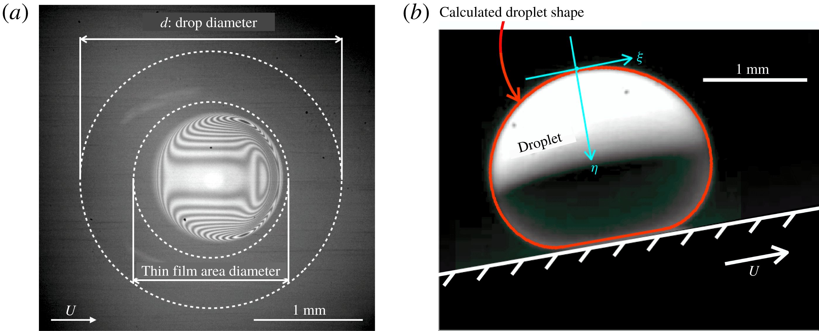
Figure 4. (a) Snapshot of interference fringes obtained by interferometric method. (b) Coordinate system for computing droplet shape for the determination of droplet mass $m$
. (Also see Saito & Tagawa Reference Saito and Tagawa2015.)
$m$
. (Also see Saito & Tagawa Reference Saito and Tagawa2015.)
Figure 5. Snapshots of interference fringes (a) under a ‘steady state’ where the minimum thickness of the air film changes within 630 nm (two fringes) over 0.05 s and (b) under an ‘unsteady state’ where the minimum thickness changes more than 630 nm. The red line is a fringe of the minimum thickness of the air film at 0 ms.
The three-dimensional shape of the air film is reconstructed from the interference fringes (Saito & Tagawa Reference Saito and Tagawa2015). In this paper, we use the terms ‘shape’ to refer to the relative distance between fringes and ‘thickness’ to refer to the absolute distance from the wall. From the fringe pattern, we obtain only the air film shape. We cannot obtain the film thickness unless we can measure the absolute thickness of the interference fringes. To obtain the absolute thickness of the fringes, we push the levitating droplet until the droplet touches the wall and record the temporal evolution of the fringes with the high-speed camera, as shown in figure 6. We calculate the absolute thickness of the air film from the number of newly generated fringes. Note that there exists an area where the film thickness is too large to obtain fringes. We interpolate the spaces between the obtained fringes and the rim of the thin film area to calculate $\unicode[STIX]{x1D705}$
using the smoothing function GRIDFIT written in MATLAB (D’Errico Reference D’Errico2006) where Triangle interpolation is used. The average error of the calculated curvature is approximately 7 % with closed fringes. The error becomes large around both ends of the opened interference fringes near the downstream rim of the thin-film area (see appendix C). We change
$\unicode[STIX]{x1D705}$
using the smoothing function GRIDFIT written in MATLAB (D’Errico Reference D’Errico2006) where Triangle interpolation is used. The average error of the calculated curvature is approximately 7 % with closed fringes. The error becomes large around both ends of the opened interference fringes near the downstream rim of the thin-film area (see appendix C). We change $U=0.73$
–
$U=0.73$
– $1.57~\text{m}~\text{s}^{-1}$
,
$1.57~\text{m}~\text{s}^{-1}$
, $\unicode[STIX]{x1D708}=100$
–
$\unicode[STIX]{x1D708}=100$
– $5000~\text{cSt}$
and
$5000~\text{cSt}$
and $d=1.17$
–
$d=1.17$
– $3.16~\text{mm}$
.
$3.16~\text{mm}$
.
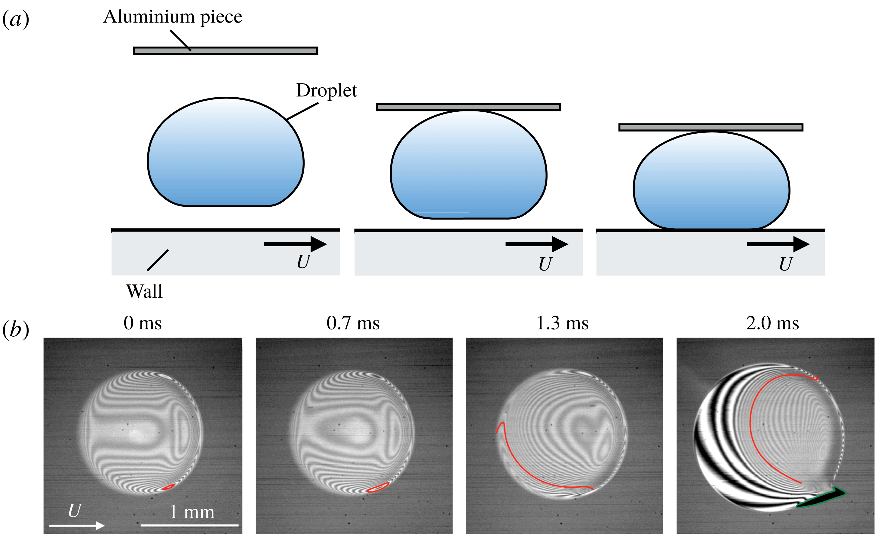
Figure 6. (a) Schematic of measurement for absolute thickness of the fringes (side view). (b) Temporal evolution of interference fringes as a levitating droplet is pushed towards a wall until it touches the wall. The red line is a fringe of the minimum thickness of the air film at 0 ms, which will attach to the wall earlier. The green line shows the location where the droplet touches the wall.
In order to compute $\unicode[STIX]{x1D703}$
, we measure an arc length of the cylinder wall from the position on the cylinder wall at
$\unicode[STIX]{x1D703}$
, we measure an arc length of the cylinder wall from the position on the cylinder wall at $\unicode[STIX]{x1D703}=0^{\circ }$
to where the droplet levitates. Droplet diameter
$\unicode[STIX]{x1D703}=0^{\circ }$
to where the droplet levitates. Droplet diameter $d$
is determined from an image of the levitating droplet projected onto the
$d$
is determined from an image of the levitating droplet projected onto the $x$
–
$x$
– $y$
surface (see figure 4
a). Since it is difficult to measure
$y$
surface (see figure 4
a). Since it is difficult to measure $m$
directly, we calculate it as follows. It is known that the levitating droplet shape agrees well with that on a fixed wall for a contact angle of
$m$
directly, we calculate it as follows. It is known that the levitating droplet shape agrees well with that on a fixed wall for a contact angle of $180^{\circ }$
for small drops only when the underlying film is not too deformed (Snoeijer, Brunet & Eggers Reference Snoeijer, Brunet and Eggers2009; Sobac et al.
Reference Sobac, Rednikov, Dorbolo and Colinet2014; Saito & Tagawa Reference Saito and Tagawa2015) (see figure 4
b). In this case, the droplet shape on a fixed wall is determined by a balance between the surface tension and hydrostatic pressures on the gas–liquid interface (Hosoma Reference Hosoma2013) in the coordinate system shown in figure 4(b):
$180^{\circ }$
for small drops only when the underlying film is not too deformed (Snoeijer, Brunet & Eggers Reference Snoeijer, Brunet and Eggers2009; Sobac et al.
Reference Sobac, Rednikov, Dorbolo and Colinet2014; Saito & Tagawa Reference Saito and Tagawa2015) (see figure 4
b). In this case, the droplet shape on a fixed wall is determined by a balance between the surface tension and hydrostatic pressures on the gas–liquid interface (Hosoma Reference Hosoma2013) in the coordinate system shown in figure 4(b):
 $$\begin{eqnarray}2\unicode[STIX]{x1D70E}\unicode[STIX]{x1D705}_{t}+\unicode[STIX]{x0394}\unicode[STIX]{x1D70C}g\unicode[STIX]{x1D702}=\unicode[STIX]{x1D70E}(\unicode[STIX]{x1D705}_{1}(\unicode[STIX]{x1D709},\unicode[STIX]{x1D702})+\unicode[STIX]{x1D705}_{2}(\unicode[STIX]{x1D709},\unicode[STIX]{x1D702})),\end{eqnarray}$$
where the first and second terms on the left-hand side stand for the surface tension pressure at the top of the droplet and variation of hydrostatic pressure, respectively. The right-hand side stands for the surface tension pressure at $(\unicode[STIX]{x1D709},\unicode[STIX]{x1D702})$
. Here,
$(\unicode[STIX]{x1D709},\unicode[STIX]{x1D702})$
. Here, $\unicode[STIX]{x1D705}_{t}$
,
$\unicode[STIX]{x1D705}_{t}$
, $\unicode[STIX]{x1D705}_{1}(\unicode[STIX]{x1D709},\unicode[STIX]{x1D702})$
and
$\unicode[STIX]{x1D705}_{1}(\unicode[STIX]{x1D709},\unicode[STIX]{x1D702})$
and $\unicode[STIX]{x1D705}_{2}(\unicode[STIX]{x1D709},\unicode[STIX]{x1D702})$
indicate the curvature at the top of the droplet, the curvature at
$\unicode[STIX]{x1D705}_{2}(\unicode[STIX]{x1D709},\unicode[STIX]{x1D702})$
indicate the curvature at the top of the droplet, the curvature at $(\unicode[STIX]{x1D709},\unicode[STIX]{x1D702})$
and the curvature normal to
$(\unicode[STIX]{x1D709},\unicode[STIX]{x1D702})$
and the curvature normal to $\unicode[STIX]{x1D705}_{t}$
, respectively. Parameters
$\unicode[STIX]{x1D705}_{t}$
, respectively. Parameters $\unicode[STIX]{x1D70E}$
and
$\unicode[STIX]{x1D70E}$
and $\unicode[STIX]{x0394}\unicode[STIX]{x1D70C}$
indicate the surface tension coefficient and the density difference between the air and the liquid, respectively. We numerically compute the droplet shape from the measured diameter
$\unicode[STIX]{x0394}\unicode[STIX]{x1D70C}$
indicate the surface tension coefficient and the density difference between the air and the liquid, respectively. We numerically compute the droplet shape from the measured diameter $d$
(see figure 4) using Mathematica and calculate
$d$
(see figure 4) using Mathematica and calculate $m$
as the product of the droplet density
$m$
as the product of the droplet density $\unicode[STIX]{x1D70C}_{d}$
and droplet volume which is obtained from the computed droplet shape. In our experiments, the droplet shape is hardly affected by the variation of the film thickness which is less than 1 % of the droplet diameter
$\unicode[STIX]{x1D70C}_{d}$
and droplet volume which is obtained from the computed droplet shape. In our experiments, the droplet shape is hardly affected by the variation of the film thickness which is less than 1 % of the droplet diameter $d$
.
$d$
.
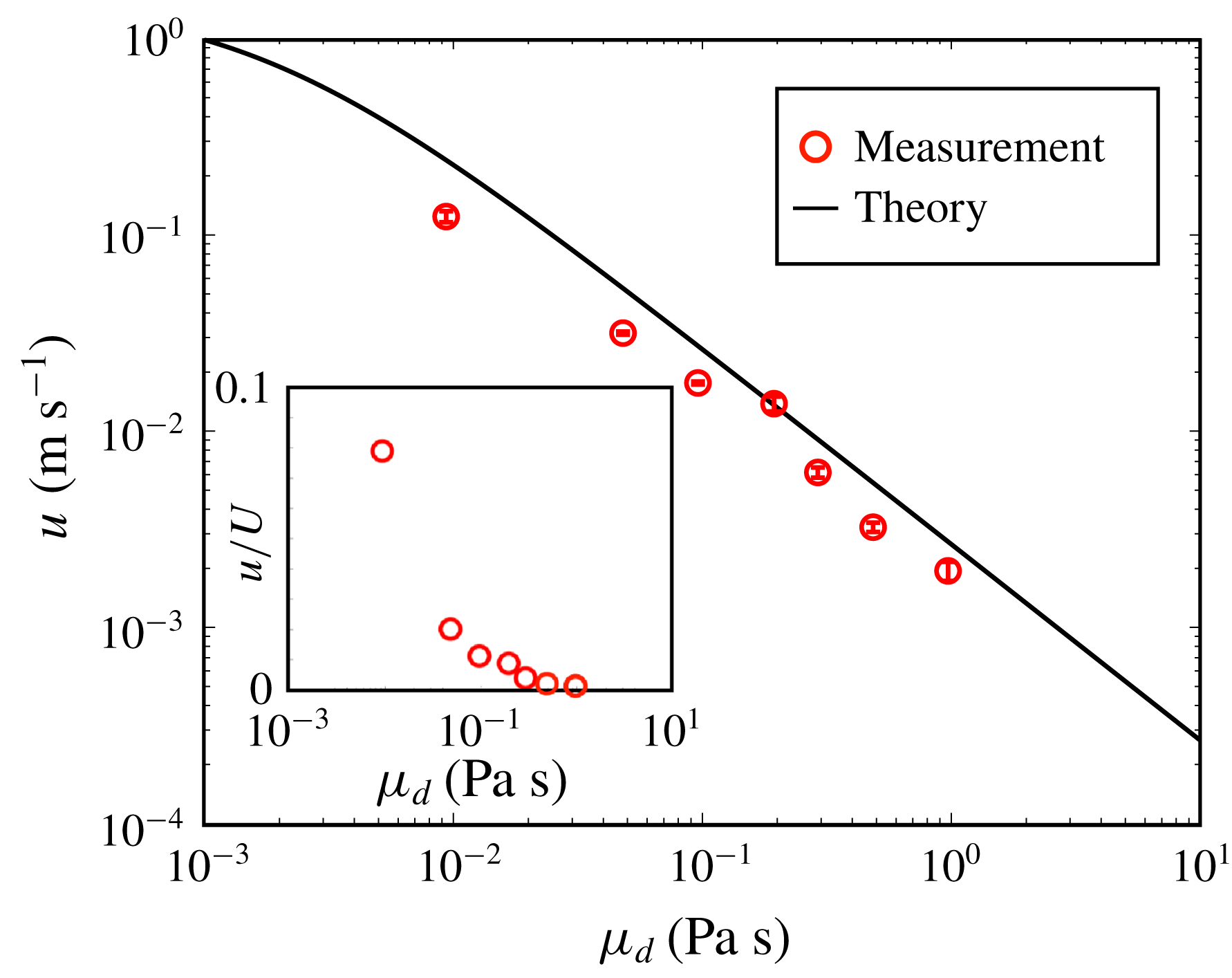
Figure 7. Surface velocity $u$
versus dynamic viscosity of droplet
$u$
versus dynamic viscosity of droplet $\unicode[STIX]{x1D707}_{d}$
. The viscosity
$\unicode[STIX]{x1D707}_{d}$
. The viscosity $\unicode[STIX]{x1D708}$
of measurement ranges from 10 to 1000 cSt, and wall velocity
$\unicode[STIX]{x1D708}$
of measurement ranges from 10 to 1000 cSt, and wall velocity $U$
is fixed at
$U$
is fixed at $1.57~\text{m}~\text{s}^{-1}$
. Error bars are the standard error. The inset shows a plot of the ratio
$1.57~\text{m}~\text{s}^{-1}$
. Error bars are the standard error. The inset shows a plot of the ratio $u/U$
as a function
$u/U$
as a function $\unicode[STIX]{x1D707}_{d}$
.
$\unicode[STIX]{x1D707}_{d}$
.
4 Effect of droplet viscosity on steady levitation
In this section, we consider the effects of the droplet viscosity on the surface velocity of the droplet $u$
and the steady state of the air film. The obtained movie and measured results of
$u$
and the steady state of the air film. The obtained movie and measured results of $u$
are shown in movie 2 and figure 7, respectively. Figure 7 shows a log–log plot where the horizontal and vertical axes represent
$u$
are shown in movie 2 and figure 7, respectively. Figure 7 shows a log–log plot where the horizontal and vertical axes represent $\unicode[STIX]{x1D707}_{d}$
and
$\unicode[STIX]{x1D707}_{d}$
and $u$
, respectively. Error bars are the standard error. The black line indicates the theoretical consideration given in (2.5) with
$u$
, respectively. Error bars are the standard error. The black line indicates the theoretical consideration given in (2.5) with $d^{\prime }=1.7~\text{mm}$
and
$d^{\prime }=1.7~\text{mm}$
and $\overline{h}=9.2~\unicode[STIX]{x03BC}\text{m}$
. Note that we assume the average thickness
$\overline{h}=9.2~\unicode[STIX]{x03BC}\text{m}$
. Note that we assume the average thickness $\overline{h}$
of the air film thickness in unsteady state to be equal to that in steady state with similar wall velocity
$\overline{h}$
of the air film thickness in unsteady state to be equal to that in steady state with similar wall velocity $U$
and droplet diameter
$U$
and droplet diameter $d$
for the following reasons. The average thickness
$d$
for the following reasons. The average thickness $\overline{h}$
in steady state is nearly independent of viscosity
$\overline{h}$
in steady state is nearly independent of viscosity $\unicode[STIX]{x1D708}$
(we discuss it in detail later in this section), and the variation of the air film thickness is about
$\unicode[STIX]{x1D708}$
(we discuss it in detail later in this section), and the variation of the air film thickness is about $\pm 2~\unicode[STIX]{x03BC}\text{m}$
in unsteady state. The value of
$\pm 2~\unicode[STIX]{x03BC}\text{m}$
in unsteady state. The value of $9.2~\unicode[STIX]{x03BC}\text{m}$
is the average thickness
$9.2~\unicode[STIX]{x03BC}\text{m}$
is the average thickness $\overline{h}$
in the steady state where the wall velocity
$\overline{h}$
in the steady state where the wall velocity $U$
and the droplet diameter
$U$
and the droplet diameter $d$
are similar to the condition of the unsteady state. The inset of figure 7 shows a plot of the ratio
$d$
are similar to the condition of the unsteady state. The inset of figure 7 shows a plot of the ratio $u/U$
as function of
$u/U$
as function of $\unicode[STIX]{x1D707}_{d}$
. Note that although the droplet shown in movie 2 appears to rotate like a rigid body, an overhead view of the droplet shows a complicated internal flow, as seen in movie 3. Thus, the net torque balance of the droplet cannot be verified experimentally. Moreover, the model does not consider prefactors seriously. Nevertheless,
$\unicode[STIX]{x1D707}_{d}$
. Note that although the droplet shown in movie 2 appears to rotate like a rigid body, an overhead view of the droplet shows a complicated internal flow, as seen in movie 3. Thus, the net torque balance of the droplet cannot be verified experimentally. Moreover, the model does not consider prefactors seriously. Nevertheless, $u$
decreases monotonically with increasing droplet viscosity for both experiments and theory with reasonable agreement. For a dynamic viscosity of
$u$
decreases monotonically with increasing droplet viscosity for both experiments and theory with reasonable agreement. For a dynamic viscosity of $\unicode[STIX]{x1D707}_{d}\geqslant 0.96\times 10^{-1}~\text{Pa}~\text{s}$
(i.e. viscosity
$\unicode[STIX]{x1D707}_{d}\geqslant 0.96\times 10^{-1}~\text{Pa}~\text{s}$
(i.e. viscosity $\unicode[STIX]{x1D708}\geqslant 100~\text{cSt}$
),
$\unicode[STIX]{x1D708}\geqslant 100~\text{cSt}$
), $u$
is less than 5 % (see inset of figure 7) of
$u$
is less than 5 % (see inset of figure 7) of $U$
. In this regime, the
$U$
. In this regime, the $L$
values calculated for the surface velocity
$L$
values calculated for the surface velocity $u$
are within the measurement error. Thus, it is reasonable to assume that
$u$
are within the measurement error. Thus, it is reasonable to assume that $u$
is negligible for
$u$
is negligible for $\unicode[STIX]{x1D708}\geqslant 100~\text{cSt}$
.
$\unicode[STIX]{x1D708}\geqslant 100~\text{cSt}$
.
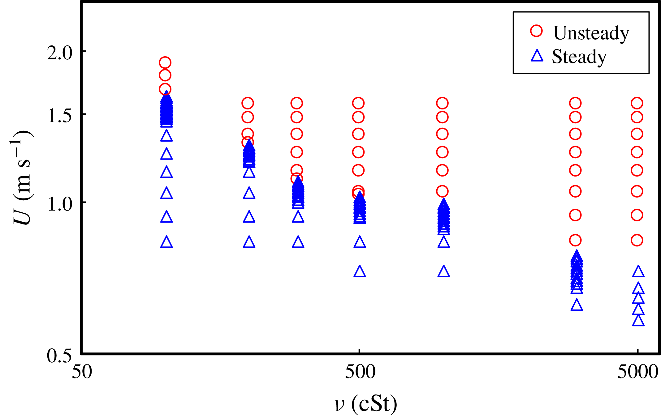
Figure 8. Air film shape under a levitating droplet with varying viscosity and wall velocity. Droplet diameter $d$
is
$d$
is $2.3\pm 0.1~\text{mm}$
.
$2.3\pm 0.1~\text{mm}$
.
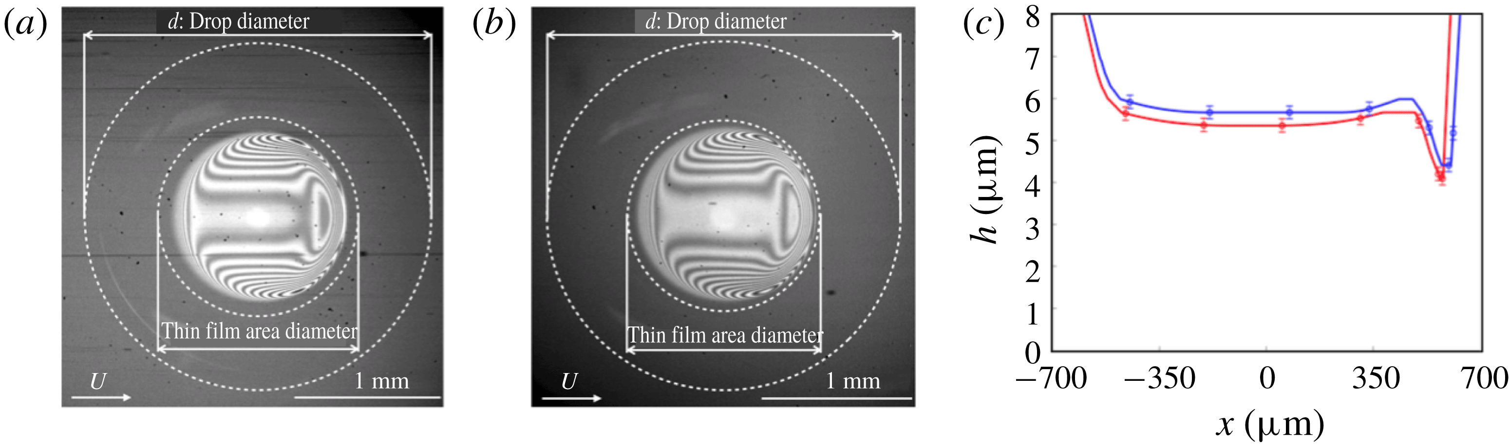
Figure 9. Snapshots of interference fringes under a levitating droplet with viscosity of (a) 500 cSt and (b) 5000 cSt. (c) Droplet shape along the symmetric axis. The blue curve and red curve correspond to the shape of the 500 cSt droplet and 5000 cSt droplet, respectively. Position $x=0$
indicates the centre of the droplet.
$x=0$
indicates the centre of the droplet.
Figure 10. (a) Air film thickness measured by the interferometric method. The arrow and black lines represent the direction of wall velocity and both interference fringes and the rim of the thin film area, respectively. We show only a part of the air film in order to emphasize the details in the thin-film area. (b) Pressure distribution calculated by applying lubrication theory. The pressure is shown in gauge pressure and the arrow and black line represent the direction of wall velocity and the rim of the thin-film area, respectively. Experimental parameters are as follows: $d=3.16\pm 0.02~\text{mm}$
,
$d=3.16\pm 0.02~\text{mm}$
, $U=1.57~\text{m}~\text{s}^{-1}$
and
$U=1.57~\text{m}~\text{s}^{-1}$
and $\unicode[STIX]{x1D708}=100~\text{cSt}$
.
$\unicode[STIX]{x1D708}=100~\text{cSt}$
.
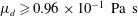
We next investigate the effect of droplet viscosity on the steady state of the air film shape. We show results of the steady state of the air film in figure 8. The blue triangles and red circles represent steady state and unsteady state, respectively. For a fixed $\unicode[STIX]{x1D708}$
, the air film shape changes from steady to unsteady as
$\unicode[STIX]{x1D708}$
, the air film shape changes from steady to unsteady as $U$
increases. For a fixed
$U$
increases. For a fixed $U$
, the air film shape changes from steady to unsteady as
$U$
, the air film shape changes from steady to unsteady as $\unicode[STIX]{x1D708}$
increases. For
$\unicode[STIX]{x1D708}$
increases. For $\unicode[STIX]{x1D708}=5000~\text{cSt}$
, the air film shape is in the steady state for
$\unicode[STIX]{x1D708}=5000~\text{cSt}$
, the air film shape is in the steady state for $U\approx 0.7~\text{m}~\text{s}^{-1}$
, which is less than half the wall velocity for the
$U\approx 0.7~\text{m}~\text{s}^{-1}$
, which is less than half the wall velocity for the $\unicode[STIX]{x1D708}=100~\text{cSt}$
case (
$\unicode[STIX]{x1D708}=100~\text{cSt}$
case ( $U\approx 1.6~\text{m}~\text{s}^{-1}$
). This indicates that the unsteady state does not originate from capillary waves since capillary waves are unlikely to be enhanced by liquid viscosity. The exact origin of the unsteady state is thus still unknown. Now, we consider the effect of droplet viscosity on the steady film shape. Figures 9(a) and 9(b) show obtained images of interference fringes under droplets with
$U\approx 1.6~\text{m}~\text{s}^{-1}$
). This indicates that the unsteady state does not originate from capillary waves since capillary waves are unlikely to be enhanced by liquid viscosity. The exact origin of the unsteady state is thus still unknown. Now, we consider the effect of droplet viscosity on the steady film shape. Figures 9(a) and 9(b) show obtained images of interference fringes under droplets with $d=2.34\pm 0.01~\text{mm}$
,
$d=2.34\pm 0.01~\text{mm}$
, $\unicode[STIX]{x1D708}=500~\text{cSt}$
and
$\unicode[STIX]{x1D708}=500~\text{cSt}$
and $U=0.73~\text{m}~\text{s}^{-1}$
, and
$U=0.73~\text{m}~\text{s}^{-1}$
, and $d=2.37\pm 0.01~\text{mm}$
,
$d=2.37\pm 0.01~\text{mm}$
, $\unicode[STIX]{x1D708}=5000~\text{cSt}$
and
$\unicode[STIX]{x1D708}=5000~\text{cSt}$
and $U=0.73~\text{m}~\text{s}^{-1}$
, respectively. The two images of interference fringes shown in figure 9(a,b) have common characteristics. For quantitative comparison, we show the shape of both droplets along the symmetric axis in figure 9(c). The difference in the film thickness is around a quarter of the wavelength of the incident light, i.e. within the measurement error of our interference method. Therefore, the droplet viscosity does not affect the film shape when the air film is in the steady state.
$U=0.73~\text{m}~\text{s}^{-1}$
, respectively. The two images of interference fringes shown in figure 9(a,b) have common characteristics. For quantitative comparison, we show the shape of both droplets along the symmetric axis in figure 9(c). The difference in the film thickness is around a quarter of the wavelength of the incident light, i.e. within the measurement error of our interference method. Therefore, the droplet viscosity does not affect the film shape when the air film is in the steady state.
The above results verify that droplet viscosity is an important factor in determining the surface velocity of a droplet and the steady state of the air film, although it does not affect the film shape kept in steady state. In the following section, we investigate the lubrication pressure under the experimental conditions where the surface velocity is negligible and the air film is in the steady state.
5 Global and local force balances
In this section, we experimentally verify two kinds of force balances. An example of the measured thickness of an air film is shown in figure 10(a) with $d=3.16\pm 0.02~\text{mm}$
,
$d=3.16\pm 0.02~\text{mm}$
, $\unicode[STIX]{x1D708}=100~\text{cSt}$
and
$\unicode[STIX]{x1D708}=100~\text{cSt}$
and $U=1.57~\text{m}~\text{s}^{-1}$
. The measured air film has a flat shape near the centre of the thin-film area and a dimple in an off-centred area. In addition, the air film has its smallest thickness in two areas near the downstream rim. A film shape having these characteristics is called a ‘horseshoe shape’, and has also been observed under other experimental conditions in our study. Note that this unique shape is also found at droplet migration in a Hele–Shaw cell (Ling et al.
Reference Ling, Fullana, Popinent and Josserand2016). Furthermore, this shape is reported in previous studies (Lhuissier et al.
Reference Lhuissier, Tagawa, Tran and Sun2013; Huerre et al.
Reference Huerre, Theodoly, Leshansky, Valignat, Cantat and Jullien2015, Reference Huerre, Jullien, Theodoly and Valignat2016; Zhu & Gallaire Reference Zhu and Gallaire2016; Daniel et al.
Reference Daniel, Timonen, Li, Velling and Aizenberg2017; Reichert et al.
Reference Reichert, Huerre, Theodoly, Valignat, Cantat and Jullien2018). Figure 10(b) shows
$U=1.57~\text{m}~\text{s}^{-1}$
. The measured air film has a flat shape near the centre of the thin-film area and a dimple in an off-centred area. In addition, the air film has its smallest thickness in two areas near the downstream rim. A film shape having these characteristics is called a ‘horseshoe shape’, and has also been observed under other experimental conditions in our study. Note that this unique shape is also found at droplet migration in a Hele–Shaw cell (Ling et al.
Reference Ling, Fullana, Popinent and Josserand2016). Furthermore, this shape is reported in previous studies (Lhuissier et al.
Reference Lhuissier, Tagawa, Tran and Sun2013; Huerre et al.
Reference Huerre, Theodoly, Leshansky, Valignat, Cantat and Jullien2015, Reference Huerre, Jullien, Theodoly and Valignat2016; Zhu & Gallaire Reference Zhu and Gallaire2016; Daniel et al.
Reference Daniel, Timonen, Li, Velling and Aizenberg2017; Reichert et al.
Reference Reichert, Huerre, Theodoly, Valignat, Cantat and Jullien2018). Figure 10(b) shows $p$
calculated by applying lubrication theory (2.1) to the film thickness shown in figure 10(a). The lubrication pressure is positive for a wide range of the thin-film area and is negative near the rim. The lubrication pressure for other experimental conditions has the same characteristics as described above.
$p$
calculated by applying lubrication theory (2.1) to the film thickness shown in figure 10(a). The lubrication pressure is positive for a wide range of the thin-film area and is negative near the rim. The lubrication pressure for other experimental conditions has the same characteristics as described above.
With the as-calculated $p$
, we investigate the global and local balances in §§ 5.1 and 5.2, respectively.
$p$
, we investigate the global and local balances in §§ 5.1 and 5.2, respectively.
5.1 Global force acting on droplet
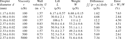
For the experimental condition presented in figure 10, the lift force $L$
generated inside the air film is calculated by (2.2) as
$L$
generated inside the air film is calculated by (2.2) as $L=(1.06\pm 0.05)\times 10^{-4}~\text{N}$
. The droplet’s weight
$L=(1.06\pm 0.05)\times 10^{-4}~\text{N}$
. The droplet’s weight $W$
is computed by (2.3) as
$W$
is computed by (2.3) as $W=(1.11\pm 0.02)\times 10^{-4}~\text{N}$
. Thus, the forces quantitatively agree within the measurement error. We show the calculated lifts and weights in table 2 under a variety of experimental conditions, changing
$W=(1.11\pm 0.02)\times 10^{-4}~\text{N}$
. Thus, the forces quantitatively agree within the measurement error. We show the calculated lifts and weights in table 2 under a variety of experimental conditions, changing $d$
,
$d$
, $\unicode[STIX]{x1D708}$
and
$\unicode[STIX]{x1D708}$
and $U$
. Note that the lift
$U$
. Note that the lift $L$
considering the surface velocity
$L$
considering the surface velocity $u$
is still within the range of the lift
$u$
is still within the range of the lift $L$
shown in table 2. Therefore, the surface velocity
$L$
shown in table 2. Therefore, the surface velocity $u$
is insignificant for the experimental conditions shown in table 2. For all conditions, we obtain quantitative agreements between the forces within the measurement error. Consequently, we have clarified that the lift force acting on the droplet generated inside the air film is balanced with the droplet’s weight when the droplet shows stable levitation over the moving wall. This confirms that the droplet levitation is sustained only by lubrication pressure and not by air drag. We show the relative difference between
$u$
is insignificant for the experimental conditions shown in table 2. For all conditions, we obtain quantitative agreements between the forces within the measurement error. Consequently, we have clarified that the lift force acting on the droplet generated inside the air film is balanced with the droplet’s weight when the droplet shows stable levitation over the moving wall. This confirms that the droplet levitation is sustained only by lubrication pressure and not by air drag. We show the relative difference between $L$
and
$L$
and $W$
in table 2 for all the experimental conditions.
$W$
in table 2 for all the experimental conditions.
Table 2. Calculated lift and weight for a variety of experimental conditions, and quantitative comparison of global and local force balances.
5.2 Local balance acting on bottom of droplet
We present distributions of $p$
(2.1) and the sum of surface tension and hydrostatic pressures
$p$
(2.1) and the sum of surface tension and hydrostatic pressures $p_{s}$
(2.4) in figures 11(a) and 11(b), respectively. The experimental condition is the case presented in figure 10. Figure 11(a) is a top view of figure 10(b). Both pressure distributions have positive values in a wide range of the thin-film area, except in the vicinity of the downstream rim. This qualitative agreement suggests that the local balance of pressure is satisfied at the bottom of the droplet.
$p_{s}$
(2.4) in figures 11(a) and 11(b), respectively. The experimental condition is the case presented in figure 10. Figure 11(a) is a top view of figure 10(b). Both pressure distributions have positive values in a wide range of the thin-film area, except in the vicinity of the downstream rim. This qualitative agreement suggests that the local balance of pressure is satisfied at the bottom of the droplet.
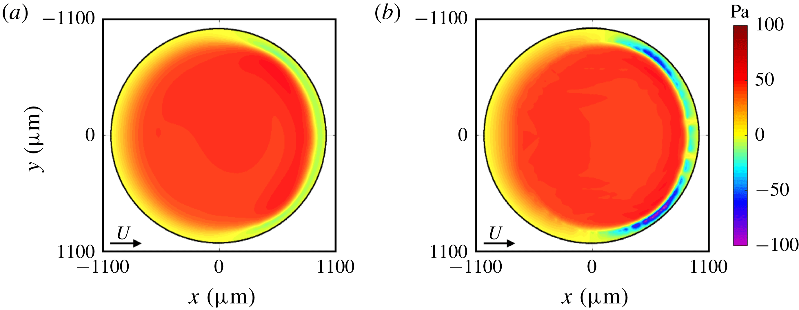
Figure 11. (a) Pressure distribution $p$
calculated by applying lubrication theory and (b) sum
$p$
calculated by applying lubrication theory and (b) sum $p_{s}$
of surface tension and hydrostatic pressures. The horizontal and vertical axes are the
$p_{s}$
of surface tension and hydrostatic pressures. The horizontal and vertical axes are the $x$
- and
$x$
- and $y$
-axes. The arrow and black line represent the direction of wall velocity and the rim of the thin-film area, respectively. Experimental parameters are as follows:
$y$
-axes. The arrow and black line represent the direction of wall velocity and the rim of the thin-film area, respectively. Experimental parameters are as follows: $d=3.16\pm 0.02~\text{mm}$
,
$d=3.16\pm 0.02~\text{mm}$
, $U=1.57~\text{m}~\text{s}^{-1}$
and
$U=1.57~\text{m}~\text{s}^{-1}$
and $\unicode[STIX]{x1D708}=100~\text{cSt}$
.
$\unicode[STIX]{x1D708}=100~\text{cSt}$
.
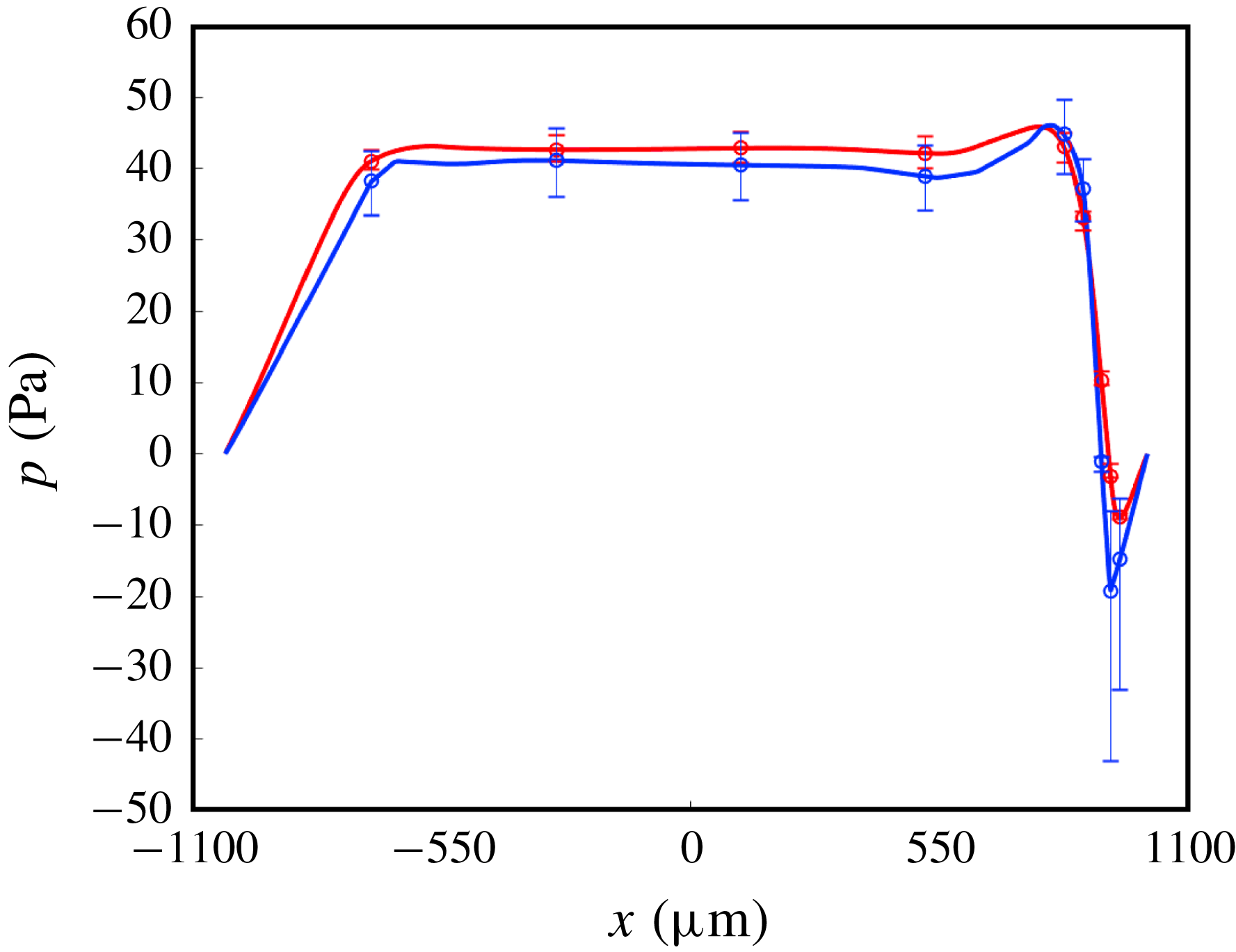
Figure 12. Cross-section of the pressure distribution $p$
calculated by applying lubrication theory (red line) and the pressure
$p$
calculated by applying lubrication theory (red line) and the pressure $p_{s}$
of surface tension and hydrostatic pressures (blue line) along
$p_{s}$
of surface tension and hydrostatic pressures (blue line) along $y=0$
. Experimental parameters are as follows:
$y=0$
. Experimental parameters are as follows: $d=3.16\pm 0.02~\text{mm}$
,
$d=3.16\pm 0.02~\text{mm}$
, $U=1.57~\text{m}~\text{s}^{-1}$
and
$U=1.57~\text{m}~\text{s}^{-1}$
and $\unicode[STIX]{x1D708}=100~\text{cSt}$
.
$\unicode[STIX]{x1D708}=100~\text{cSt}$
.
For a quantitative comparison, figure 12 shows cross-sections of the pressure distributions along $y=0$
with the measurement error. The measurement error of the pressure
$y=0$
with the measurement error. The measurement error of the pressure $p$
comes from the error of the interference method (
$p$
comes from the error of the interference method ( $\pm 1/4$
wavelength). The error of
$\pm 1/4$
wavelength). The error of $p_{s}$
comes from the error of the mean curvature
$p_{s}$
comes from the error of the mean curvature $\unicode[STIX]{x1D705}$
as well as surface tension
$\unicode[STIX]{x1D705}$
as well as surface tension $\unicode[STIX]{x1D70E}$
. The detailed error estimation process of the mean curvature
$\unicode[STIX]{x1D70E}$
. The detailed error estimation process of the mean curvature $\unicode[STIX]{x1D705}$
is shown in appendix D. The large error at negative pressure is due to the error of the mean curvature
$\unicode[STIX]{x1D705}$
is shown in appendix D. The large error at negative pressure is due to the error of the mean curvature $\unicode[STIX]{x1D705}$
. The measurement error of the surface tension
$\unicode[STIX]{x1D705}$
. The measurement error of the surface tension $\unicode[STIX]{x1D70E}$
with viscosity
$\unicode[STIX]{x1D70E}$
with viscosity $\unicode[STIX]{x1D708}=100~\text{cSt}$
is
$\unicode[STIX]{x1D708}=100~\text{cSt}$
is $\pm 0.18~\text{mN}~\text{m}^{-1}$
(9 %). The Wilhelmy method (plate method or vertical plate method) was used to determine the surface tension (CBVP-AB, Kyowa Interface Science Co.).
$\pm 0.18~\text{mN}~\text{m}^{-1}$
(9 %). The Wilhelmy method (plate method or vertical plate method) was used to determine the surface tension (CBVP-AB, Kyowa Interface Science Co.).
Notably, the overall pressure distributions for both cases are almost identical, except for the negative pressure region around $x=950~\unicode[STIX]{x03BC}\text{m}$
. For
$x=950~\unicode[STIX]{x03BC}\text{m}$
. For $-650~\unicode[STIX]{x03BC}\text{m}\leqslant x\leqslant 550~\unicode[STIX]{x03BC}\text{m}$
, the pressures are positive and nearly constant. The maximum pressures are at around
$-650~\unicode[STIX]{x03BC}\text{m}\leqslant x\leqslant 550~\unicode[STIX]{x03BC}\text{m}$
, the pressures are positive and nearly constant. The maximum pressures are at around $x=750~\unicode[STIX]{x03BC}\text{m}$
and the minimum pressures are at around
$x=750~\unicode[STIX]{x03BC}\text{m}$
and the minimum pressures are at around $x=950~\unicode[STIX]{x03BC}\text{m}$
. The difference in negative pressures is observed not only along
$x=950~\unicode[STIX]{x03BC}\text{m}$
. The difference in negative pressures is observed not only along $y=0$
but also near the rim of the thin-film area. In particular, the largest difference in negative pressure is at around
$y=0$
but also near the rim of the thin-film area. In particular, the largest difference in negative pressure is at around $(x,y)=(600~\unicode[STIX]{x03BC}\text{m},\pm 800~\unicode[STIX]{x03BC}\text{m})$
where the air film is the thinnest. The reason for this would be as follows. The surface tension pressure of the first term on the left-hand side in (2.4) is
$(x,y)=(600~\unicode[STIX]{x03BC}\text{m},\pm 800~\unicode[STIX]{x03BC}\text{m})$
where the air film is the thinnest. The reason for this would be as follows. The surface tension pressure of the first term on the left-hand side in (2.4) is $O(10^{1})$
while the hydrostatic pressure of the second term is
$O(10^{1})$
while the hydrostatic pressure of the second term is $O(10^{-2})$
and therefore the surface tension pressure dominates the sum pressure
$O(10^{-2})$
and therefore the surface tension pressure dominates the sum pressure $p_{s}$
, which is to say that the surface tension coefficient
$p_{s}$
, which is to say that the surface tension coefficient $\unicode[STIX]{x1D70E}$
and mean curvature
$\unicode[STIX]{x1D70E}$
and mean curvature $\unicode[STIX]{x1D705}$
are dominant factors for
$\unicode[STIX]{x1D705}$
are dominant factors for $p_{s}$
. A limitation of our method, as stated in § 3, is that the calculation error of curvature is especially large near both ends of the opened interference fringes. Several open ends of the interference fringes exist around the thinnest film regions, and thus the error of negative pressure is particularly large there.
$p_{s}$
. A limitation of our method, as stated in § 3, is that the calculation error of curvature is especially large near both ends of the opened interference fringes. Several open ends of the interference fringes exist around the thinnest film regions, and thus the error of negative pressure is particularly large there.
We compare $p$
and
$p$
and $p_{s}$
for a variety of experimental conditions and obtain quantitative agreement except for the values of negative pressure, namely, except for where our method exhibits limitations. We experimentally find that
$p_{s}$
for a variety of experimental conditions and obtain quantitative agreement except for the values of negative pressure, namely, except for where our method exhibits limitations. We experimentally find that $p$
locally balances with the surface tension and hydrostatic pressures at the bottom of the droplet in our experimental conditions. We show the difference of pressure
$p$
locally balances with the surface tension and hydrostatic pressures at the bottom of the droplet in our experimental conditions. We show the difference of pressure $\iint |p-p_{s}|\,\text{d}x\,\text{d}y$
in table 2 for all experimental conditions. The
$\iint |p-p_{s}|\,\text{d}x\,\text{d}y$
in table 2 for all experimental conditions. The $\iint |p-p_{s}|\,\text{d}x\,\text{d}y$
is less than three times the error of the lift
$\iint |p-p_{s}|\,\text{d}x\,\text{d}y$
is less than three times the error of the lift $L$
. Recall that
$L$
. Recall that $\iint |p-p_{s}|\,\text{d}x\,\text{d}y$
is the sum of the absolute value of difference between the pressure
$\iint |p-p_{s}|\,\text{d}x\,\text{d}y$
is the sum of the absolute value of difference between the pressure $p$
and
$p$
and $p_{s}$
while the error of the lift
$p_{s}$
while the error of the lift $L$
is calculated considering positive/negative pressure. Therefore, we regard the values
$L$
is calculated considering positive/negative pressure. Therefore, we regard the values $\iint |p-p_{s}|\,\text{d}x\,\text{d}y$
obtained in our experiments as reasonably small.
$\iint |p-p_{s}|\,\text{d}x\,\text{d}y$
obtained in our experiments as reasonably small.
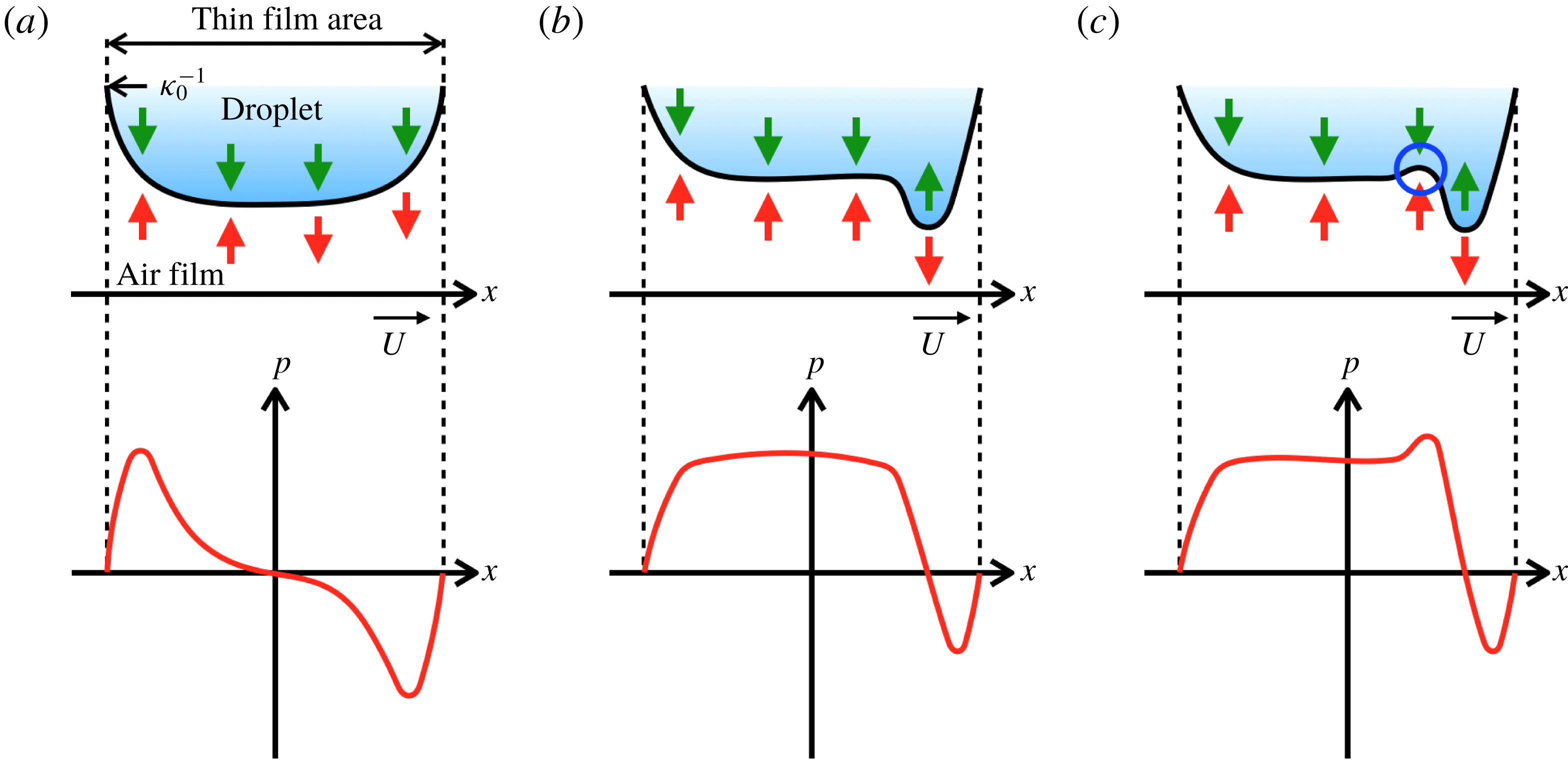
Figure 13. Schematic views of the process of air film shape formation along with the lubrication pressure and surface tension pressure in two dimensions. Upper: the gas–liquid surface shape shown as a black line, direction of lubrication pressure shown as red arrows and direction of surface tension pressure shown as green arrows. Lower: lubrication pressure. (a) Lubrication pressure has positive pressure upstream and negative pressure downstream while the surface tension pressure has positive pressure over the whole range. (b) The gas–liquid surface has a plateau in the centre of the droplet and a minimum thickness downstream. (c) A high lubrication pressure due to the steep surface region (wedge effect) arises by decreasing the air film thickness in the downstream side, and the pressure increases at the blue circle. As a result, dimple formation is generated.
5.3 Determining process of the steady horseshoe shape
In this section, we discuss how the horseshoe shape of the air film is created based on the local balance at the gas–liquid surface. We consider only the lubrication pressure and surface tension pressure, because the hydrostatic pressure is sufficiently small as mentioned in § 5.2. We first discuss the formation of the film shape in two dimensions and then expand the discussion to three dimensions.
We here outline a typical process of air film shape formation in two dimensions in the mainstream direction. Figure 13 shows schematic views of the process of the gas–liquid interface shape formation and the pressure distribution along the $x$
-axis. The surface tension pressure in figure 13 signifies
$x$
-axis. The surface tension pressure in figure 13 signifies $2\unicode[STIX]{x1D70E}(\unicode[STIX]{x1D705}_{0}-\unicode[STIX]{x1D705})$
(the first term on the left-hand side of (2.4)). As shown in figure 13(a), when the axisymmetric droplet approaches the moving wall, the lubrication pressure is positive upstream and negative downstream (Hicks & Purvis Reference Hicks and Purvis2010). The
$2\unicode[STIX]{x1D70E}(\unicode[STIX]{x1D705}_{0}-\unicode[STIX]{x1D705})$
(the first term on the left-hand side of (2.4)). As shown in figure 13(a), when the axisymmetric droplet approaches the moving wall, the lubrication pressure is positive upstream and negative downstream (Hicks & Purvis Reference Hicks and Purvis2010). The $x$
-intercept of the pressure curve is 0. Upstream, a positive lubrication pressure pushes up the gas–liquid surface, while downstream negative lubrication pressure pulls down the surface. The surface shape becomes inclined and the positive lubrication pressure region expands, i.e. the
$x$
-intercept of the pressure curve is 0. Upstream, a positive lubrication pressure pushes up the gas–liquid surface, while downstream negative lubrication pressure pulls down the surface. The surface shape becomes inclined and the positive lubrication pressure region expands, i.e. the $x$
-intercept shifts to a positive value. The negative lubrication pressure region narrows, resulting in an increase in the surface curvature near the downstream rim (see figure 13
b). This is likely why the minimum thickness is distributed near the downstream rim. The thin film downstream, around the blue circle in figure 13(c), experiences a high lubrication pressure due to the steep surface region (wedge effect), leading to dimple formation. When a negative lubrication pressure balances the surface tension pressure, the droplet can levitate without touching the moving wall.
$x$
-intercept shifts to a positive value. The negative lubrication pressure region narrows, resulting in an increase in the surface curvature near the downstream rim (see figure 13
b). This is likely why the minimum thickness is distributed near the downstream rim. The thin film downstream, around the blue circle in figure 13(c), experiences a high lubrication pressure due to the steep surface region (wedge effect), leading to dimple formation. When a negative lubrication pressure balances the surface tension pressure, the droplet can levitate without touching the moving wall.
Next, we consider the positions where the air film has the smallest thickness, around $(x,y)=(600~\unicode[STIX]{x03BC}\text{m},\pm 800~\unicode[STIX]{x03BC}\text{m})$
, as shown in figure 10(a). In the case of large absolute value of
$(x,y)=(600~\unicode[STIX]{x03BC}\text{m},\pm 800~\unicode[STIX]{x03BC}\text{m})$
, as shown in figure 10(a). In the case of large absolute value of $y$
, the positive pressure is smaller near the rim than in the centre since the boundary of the thin-film area, where atmospheric pressure is applied, is closer. This small positive pressure results in lateral (
$y$
, the positive pressure is smaller near the rim than in the centre since the boundary of the thin-film area, where atmospheric pressure is applied, is closer. This small positive pressure results in lateral ( $y$
-axis direction) suction which causes the thin-film area near the rim (a more elaborate discussion of a droplet in a liquid in a Hele–Shaw cell is found in Reichert et al.
Reference Reichert, Huerre, Theodoly, Valignat, Cantat and Jullien2018). In addition, the air flow moves the minimum thickness area in the downstream direction (Burgess & Foster Reference Burgess and Foster1990). This local pressure balance and the movement of the minimum thickness might produce the horseshoe shape of the air film, with two areas of minimum thickness near the downstream rim.
$y$
-axis direction) suction which causes the thin-film area near the rim (a more elaborate discussion of a droplet in a liquid in a Hele–Shaw cell is found in Reichert et al.
Reference Reichert, Huerre, Theodoly, Valignat, Cantat and Jullien2018). In addition, the air flow moves the minimum thickness area in the downstream direction (Burgess & Foster Reference Burgess and Foster1990). This local pressure balance and the movement of the minimum thickness might produce the horseshoe shape of the air film, with two areas of minimum thickness near the downstream rim.
6 Conclusion
Our purpose is to investigate levitating droplets over a moving wall for a wide range of experimental parameters, which have not been covered by previous studies. We experimentally measure the surface velocity of droplets and the three-dimensional shapes of the air film. The droplet viscosity is found to affect the surface velocity of a droplet and the steady state of the air film shape. An increase in droplet viscosity decreases the surface velocity, which is sufficiently small compared to the wall velocity $U$
in our experimental conditions. Droplet viscosity and wall velocity decide the steady/unsteady state of the air film. Surprisingly, increasing the droplet viscosity tends to reduce the range of velocity of the steady state. However, the film shape in the steady state is not affected by droplet viscosity. Next, for a negligible surface speed and when the steady state of the air film shape can be assumed, we calculate the pressure distribution by applying lubrication theory to the measured air film. Based on the calculated pressure distribution, we verify two kinds of balances acting on the levitating droplet, a global balance and a local balance. First, we calculate both the lift force
$U$
in our experimental conditions. Droplet viscosity and wall velocity decide the steady/unsteady state of the air film. Surprisingly, increasing the droplet viscosity tends to reduce the range of velocity of the steady state. However, the film shape in the steady state is not affected by droplet viscosity. Next, for a negligible surface speed and when the steady state of the air film shape can be assumed, we calculate the pressure distribution by applying lubrication theory to the measured air film. Based on the calculated pressure distribution, we verify two kinds of balances acting on the levitating droplet, a global balance and a local balance. First, we calculate both the lift force $L$
and the droplet’s weight
$L$
and the droplet’s weight $W$
and then compare the two values. With varying droplet diameter, viscosity and wall velocity as experimental parameters, we obtain quantitative agreement between
$W$
and then compare the two values. With varying droplet diameter, viscosity and wall velocity as experimental parameters, we obtain quantitative agreement between $L$
and
$L$
and $W$
. Thus, we experimentally verify that the lift acting on a levitating droplet balances with the droplet’s weight. Second, we calculate the surface tension and hydrostatic pressures acting on the bottom of a droplet. For all experimental conditions, we confirm the local pressure balance between lubrication pressure, surface tension and hydrostatic pressures at every point in the thin-film area, except an area with large measurement error. Thus, we experimentally verify that the local balance of pressure is satisfied at the bottom of the droplet. Finally, we consider the typical process through which the air film takes on a horseshoe shape.
$W$
. Thus, we experimentally verify that the lift acting on a levitating droplet balances with the droplet’s weight. Second, we calculate the surface tension and hydrostatic pressures acting on the bottom of a droplet. For all experimental conditions, we confirm the local pressure balance between lubrication pressure, surface tension and hydrostatic pressures at every point in the thin-film area, except an area with large measurement error. Thus, we experimentally verify that the local balance of pressure is satisfied at the bottom of the droplet. Finally, we consider the typical process through which the air film takes on a horseshoe shape.
The results obtained in this research, including the experimental evidence for the force/pressure balances, should contribute to studies of various levitating droplets, such as those over a heated surface (Lagubeau et al. Reference Lagubeau, Le Merrer, Clanet and Quéré2011; Burton et al. Reference Burton, Sharpe, Van Der Veen, Franco and Nagel2012; Tran et al. Reference Tran, Staat, Prosperetti, Sun and Lohse2012; Quéré Reference Quéré2013; Sobac et al. Reference Sobac, Rednikov, Dorbolo and Colinet2014), although droplet evaporation may add another layer of difficulty.
Acknowledgements
We thank S. Komaya and A. Franco-Gómez for their helpful contributions. This work was supported by JSPS KAKENHI grant nos. 26709007 and 17H01246.
Supplementary movies
Supplementary movies are available at https://doi.org/10.1017/jfm.2018.952.
Appendix A. Application of lubrication theory to an air film under a levitating droplet
Applying lubrication theory to a levitating droplet in the same way as in previous studies (Lhuissier et al.
Reference Lhuissier, Tagawa, Tran and Sun2013; Saito & Tagawa Reference Saito and Tagawa2015) requires a Reynolds number $Re$
inside the air film sufficiently smaller than 1 and a film thickness that is sufficiently thinner than the characteristic length along the mainstream. In this paper,
$Re$
inside the air film sufficiently smaller than 1 and a film thickness that is sufficiently thinner than the characteristic length along the mainstream. In this paper, $Re$
including a geometrical aspect ratio (
$Re$
including a geometrical aspect ratio ( $=\unicode[STIX]{x1D70C}Uh^{2}/\unicode[STIX]{x1D707}d$
) is used, and
$=\unicode[STIX]{x1D70C}Uh^{2}/\unicode[STIX]{x1D707}d$
) is used, and $Re$
is sufficiently smaller than 1 for the airflow under a levitating droplet in our experiments. Thus, it is appropriate to apply lubrication theory to the air film under a levitating droplet. However, if general
$Re$
is sufficiently smaller than 1 for the airflow under a levitating droplet in our experiments. Thus, it is appropriate to apply lubrication theory to the air film under a levitating droplet. However, if general $Re=\unicode[STIX]{x1D70C}Uh/\unicode[STIX]{x1D707}$
is used,
$Re=\unicode[STIX]{x1D70C}Uh/\unicode[STIX]{x1D707}$
is used, $Re$
is not sufficiently smaller than 1 in our experiments. Hence, it is questionable whether lubrication theory can be applied since the inertia term in the Navier–Stokes equation does not seem to be negligible. Therefore, we discuss here whether lubrication theory can be applied to the air film under a levitating droplet by performing numerical simulations. For this discussion, we numerically solve the Navier–Stokes equation including or neglecting the inertia term with a continuity equation, and then compare the pressure distributions in the air film.
$Re$
is not sufficiently smaller than 1 in our experiments. Hence, it is questionable whether lubrication theory can be applied since the inertia term in the Navier–Stokes equation does not seem to be negligible. Therefore, we discuss here whether lubrication theory can be applied to the air film under a levitating droplet by performing numerical simulations. For this discussion, we numerically solve the Navier–Stokes equation including or neglecting the inertia term with a continuity equation, and then compare the pressure distributions in the air film.
We conduct the numerical simulation using COMSOL Multiphysics, which performs computations by the finite element method. We investigate whether the inertia term affects the pressure distribution generated inside the air film based on the results of numerical simulations obtained by two kinds of governing equations: (i) the general Navier–Stokes equation and continuity equation and (ii) the Navier–Stokes equation neglecting the inertia term and continuity equation. For each approach, we use about 700 000 triangle-shape meshes. We simulate an air film between a moving wall and the three-dimensional shape of the air film as measured in our experiment with droplet diameter $d=3.16\pm 0.02~\text{mm}$
, viscosity
$d=3.16\pm 0.02~\text{mm}$
, viscosity $\unicode[STIX]{x1D708}=100~\text{cSt}$
and wall velocity
$\unicode[STIX]{x1D708}=100~\text{cSt}$
and wall velocity $U=1.57~\text{m}~\text{s}^{-1}$
. We assume that the gas–liquid interface is a solid wall with a no-slip condition since the air film has a steady shape and the surface velocity of the droplet is negligible in comparison with the wall velocity (see § 4). We use
$U=1.57~\text{m}~\text{s}^{-1}$
. We assume that the gas–liquid interface is a solid wall with a no-slip condition since the air film has a steady shape and the surface velocity of the droplet is negligible in comparison with the wall velocity (see § 4). We use $U=1.57~\text{m}~\text{s}^{-1}$
for the moving wall along the
$U=1.57~\text{m}~\text{s}^{-1}$
for the moving wall along the $x$
-axis positive direction and atmospheric pressure on the rim of the thin-film area as boundary conditions, as in our experiment.
$x$
-axis positive direction and atmospheric pressure on the rim of the thin-film area as boundary conditions, as in our experiment.
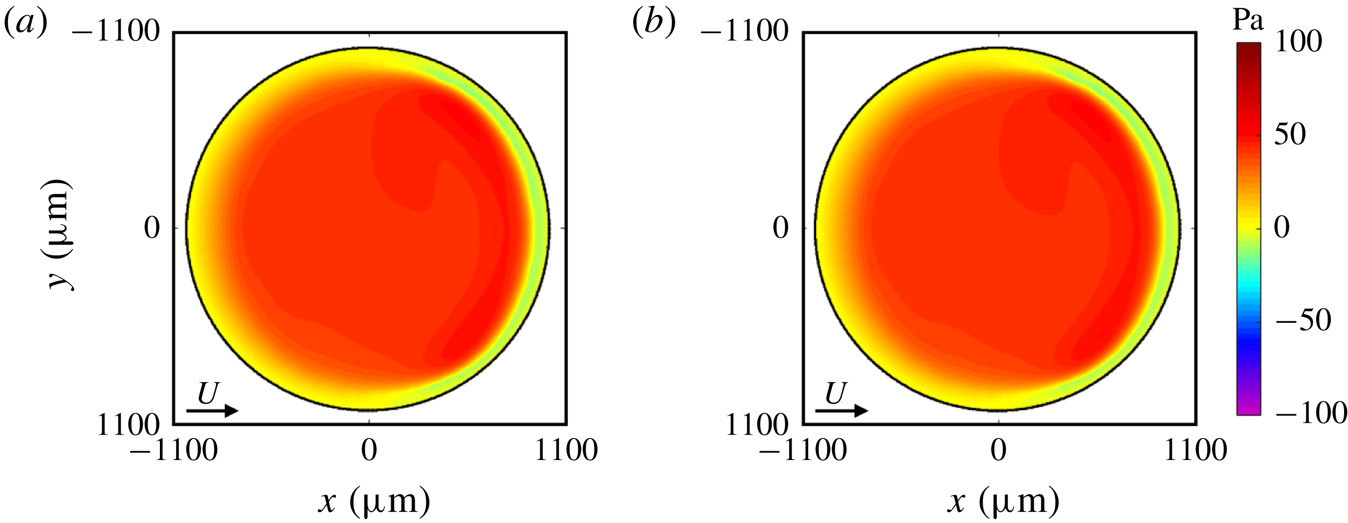
Figure 14. Pressure distribution computed by (a) general Navier–Stokes equation and continuity equation and (b) Navier–Stokes equation neglecting the inertia term and continuity equation.
Figures 14(a) and 14(b) show the pressure distributions numerically simulated by the governing equations (i) and (ii), respectively, where the horizontal and vertical axes are the $x$
- and
$x$
- and $y$
-axes and the arrow and black line represent the direction of wall velocity and the rim of the thin-film area, respectively. Both pressure distributions have positive pressure except in the vicinity of the rim of the thin-film area. The peak values of the positive and negative pressures each agree between the two distributions within an error of 0.3 %. In addition,
$y$
-axes and the arrow and black line represent the direction of wall velocity and the rim of the thin-film area, respectively. Both pressure distributions have positive pressure except in the vicinity of the rim of the thin-film area. The peak values of the positive and negative pressures each agree between the two distributions within an error of 0.3 %. In addition, $L$
calculated by (2.2) agrees for both distributions within an error of 0.3 %. Therefore, we obtain quantitative agreement between the two pressure distributions shown in figure 14(a,b). This agreement indicates that the inertia term in the Navier–Stokes equation does not largely affect the lubrication pressure.
$L$
calculated by (2.2) agrees for both distributions within an error of 0.3 %. Therefore, we obtain quantitative agreement between the two pressure distributions shown in figure 14(a,b). This agreement indicates that the inertia term in the Navier–Stokes equation does not largely affect the lubrication pressure.
Appendix B. The propagation of errors from the experimental parameters
We have the following two equations, namely for pressure gradients in the direction of $x$
-axis and
$x$
-axis and $y$
-axis to derive the equation of motion in the air film (2.1):
$y$
-axis to derive the equation of motion in the air film (2.1):
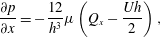 $$\begin{eqnarray}\displaystyle & \displaystyle \frac{\unicode[STIX]{x2202}p}{\unicode[STIX]{x2202}x}=-\frac{12}{h^{3}}\unicode[STIX]{x1D707}\left(Q_{x}-\frac{Uh}{2}\right), & \displaystyle\end{eqnarray}$$
 $$\begin{eqnarray}\displaystyle & \displaystyle \frac{\unicode[STIX]{x2202}p}{\unicode[STIX]{x2202}y}=-\frac{12}{h^{3}}\unicode[STIX]{x1D707}Q_{y}, & \displaystyle\end{eqnarray}$$
where $Q_{x}$
and
$Q_{x}$
and $Q_{y}$
indicate flow rate per unit thickness in the direction of
$Q_{y}$
indicate flow rate per unit thickness in the direction of $x$
-axis and
$x$
-axis and $y$
-axis, respectively. By the law of propagation of errors, the errors of pressure gradients in the direction of
$y$
-axis, respectively. By the law of propagation of errors, the errors of pressure gradients in the direction of $x$
-axis
$x$
-axis $\unicode[STIX]{x1D70E}_{x}$
and
$\unicode[STIX]{x1D70E}_{x}$
and $y$
-axis
$y$
-axis $\unicode[STIX]{x1D70E}_{y}$
from (B 1) and (B 2) are
$\unicode[STIX]{x1D70E}_{y}$
from (B 1) and (B 2) are
 $$\begin{eqnarray}\displaystyle \unicode[STIX]{x1D70E}_{x}^{2} & = & \displaystyle \left(\frac{12}{h^{3}}\unicode[STIX]{x1D707}\left(\frac{3}{h}Q_{x}-U\right)\right)^{2}\unicode[STIX]{x1D70E}_{h}^{2}+\left(-\frac{12}{h^{3}}\unicode[STIX]{x1D707}\right)^{2}\unicode[STIX]{x1D70E}_{Q_{x}}^{2}\nonumber\\ \displaystyle & & \displaystyle +\,\left(\frac{6}{h^{2}}\unicode[STIX]{x1D707}\right)^{2}\unicode[STIX]{x1D70E}_{U}^{2}+\left(-\frac{6}{h^{2}}\left(\frac{2}{h}Q_{x}-U\right)\right)^{2}\unicode[STIX]{x1D70E}_{\unicode[STIX]{x1D707}}^{2},\end{eqnarray}$$
 $$\begin{eqnarray}\unicode[STIX]{x1D70E}_{y}^{2}=\left(\frac{36}{h^{4}}\unicode[STIX]{x1D707}Q_{y}\right)^{2}\unicode[STIX]{x1D70E}_{h}^{2}+\left(-\frac{12}{h^{3}}\unicode[STIX]{x1D707}\right)^{2}\unicode[STIX]{x1D70E}_{Q_{y}}^{2}+\left(-\frac{12}{h^{3}}Q_{y}\right)^{2}\unicode[STIX]{x1D70E}_{\unicode[STIX]{x1D707}}^{2},\end{eqnarray}$$
where $\unicode[STIX]{x1D70E}_{Q_{x}}$
,
$\unicode[STIX]{x1D70E}_{Q_{x}}$
, $\unicode[STIX]{x1D70E}_{Q_{y}}$
,
$\unicode[STIX]{x1D70E}_{Q_{y}}$
, $\unicode[STIX]{x1D70E}_{\unicode[STIX]{x1D707}}$
,
$\unicode[STIX]{x1D70E}_{\unicode[STIX]{x1D707}}$
, $\unicode[STIX]{x1D70E}_{h}$
and
$\unicode[STIX]{x1D70E}_{h}$
and $\unicode[STIX]{x1D70E}_{U}$
indicate the errors of each parameter, respectively. We estimate that the air film thickness
$\unicode[STIX]{x1D70E}_{U}$
indicate the errors of each parameter, respectively. We estimate that the air film thickness $h$
, the dynamic viscosity of the air
$h$
, the dynamic viscosity of the air $\unicode[STIX]{x1D707}$
and the wall velocity
$\unicode[STIX]{x1D707}$
and the wall velocity $U$
are
$U$
are $O(10^{-6})~\text{m}$
,
$O(10^{-6})~\text{m}$
, $O(10^{-5})~\text{Pa}~\text{s}$
and
$O(10^{-5})~\text{Pa}~\text{s}$
and $O(10^{0})~\text{m}$
, respectively. The flow rate
$O(10^{0})~\text{m}$
, respectively. The flow rate $Q_{x}$
is
$Q_{x}$
is $O(10^{-6})~\text{m}^{2}~\text{s}^{-1}$
which comes from the wall velocity
$O(10^{-6})~\text{m}^{2}~\text{s}^{-1}$
which comes from the wall velocity $U$
and the air film thickness
$U$
and the air film thickness $h$
. We also estimate that
$h$
. We also estimate that $\unicode[STIX]{x1D70E}_{h}$
,
$\unicode[STIX]{x1D70E}_{h}$
, $\unicode[STIX]{x1D70E}_{\unicode[STIX]{x1D707}}$
and
$\unicode[STIX]{x1D70E}_{\unicode[STIX]{x1D707}}$
and $\unicode[STIX]{x1D70E}_{U}$
are
$\unicode[STIX]{x1D70E}_{U}$
are $O(10^{-6})~\text{m}$
,
$O(10^{-6})~\text{m}$
, $O(10^{-7})~\text{Pa}~\text{s}$
and
$O(10^{-7})~\text{Pa}~\text{s}$
and $O(10^{-2})~\text{m}$
, respectively. Error
$O(10^{-2})~\text{m}$
, respectively. Error $\unicode[STIX]{x1D70E}_{Q_{x}}$
is
$\unicode[STIX]{x1D70E}_{Q_{x}}$
is $O(10^{-2})~\text{m}^{2}~\text{s}^{-1}$
which is same as
$O(10^{-2})~\text{m}^{2}~\text{s}^{-1}$
which is same as $\unicode[STIX]{x1D70E}_{U}$
, because
$\unicode[STIX]{x1D70E}_{U}$
, because $\unicode[STIX]{x1D70E}_{h}$
is sufficiently small in comparison with
$\unicode[STIX]{x1D70E}_{h}$
is sufficiently small in comparison with $\unicode[STIX]{x1D70E}_{U}$
. The flow rate
$\unicode[STIX]{x1D70E}_{U}$
. The flow rate $Q_{y}$
is assumed to be negligible. As a result, we find that the error of the air film thickness
$Q_{y}$
is assumed to be negligible. As a result, we find that the error of the air film thickness $h$
is dominant in comparison with those of the other parameters.
$h$
is dominant in comparison with those of the other parameters.
Appendix C. Decision procedure of the thin-film area
We consider the area inside the air film where the lubrication pressure is generated as the thin-film area. The rim of the thin-film area has thickness $H$
which is equal to
$H$
which is equal to $z_{0}$
(see figure 2) and experiences atmospheric pressure as the boundary condition. When
$z_{0}$
(see figure 2) and experiences atmospheric pressure as the boundary condition. When $H$
changes with the thin-film area diameter
$H$
changes with the thin-film area diameter $d_{t}$
, the thin-film area where the lubrication theory is applied also changes. Therefore, we need to select the proper thickness
$d_{t}$
, the thin-film area where the lubrication theory is applied also changes. Therefore, we need to select the proper thickness $H$
to accurately calculate the lubrication pressure
$H$
to accurately calculate the lubrication pressure $p$
generated inside the air film. In this appendix, we determine the thin-film area and the thickness at its rim
$p$
generated inside the air film. In this appendix, we determine the thin-film area and the thickness at its rim $H$
focusing on the lift
$H$
focusing on the lift $L$
. We calculate
$L$
. We calculate $L$
for a range of thicknesses
$L$
for a range of thicknesses $H$
, in steps of
$H$
, in steps of $1~\unicode[STIX]{x03BC}\text{m}$
. When the variation of
$1~\unicode[STIX]{x03BC}\text{m}$
. When the variation of $L$
with
$L$
with $H$
is smaller than the measurement error, that value of
$H$
is smaller than the measurement error, that value of $H$
is defined as the thickness of the thin-film area. Next, we numerically compute
$H$
is defined as the thickness of the thin-film area. Next, we numerically compute $d_{t}$
corresponding to each value of
$d_{t}$
corresponding to each value of $H$
.
$H$
.
We show an example of our results in figure 15, where the horizontal axis is the thickness at the rim of the thin-film area, $H$
, and the vertical axis is the calculated
$H$
, and the vertical axis is the calculated $L$
. The result is obtained for a droplet diameter of
$L$
. The result is obtained for a droplet diameter of $d=3.16\pm 0.02~\text{mm}$
, viscosity
$d=3.16\pm 0.02~\text{mm}$
, viscosity $\unicode[STIX]{x1D708}=100~\text{cSt}$
and wall velocity
$\unicode[STIX]{x1D708}=100~\text{cSt}$
and wall velocity $U=1.57~\text{m}~\text{s}^{-1}$
. The variation in
$U=1.57~\text{m}~\text{s}^{-1}$
. The variation in $L$
is smaller than 1 % when
$L$
is smaller than 1 % when $H$
is in the range
$H$
is in the range $20$
–
$20$
– $24~\unicode[STIX]{x03BC}\text{m}$
. However, the measurement error of the calculated
$24~\unicode[STIX]{x03BC}\text{m}$
. However, the measurement error of the calculated $L$
is 5 % for
$L$
is 5 % for $H=22~\unicode[STIX]{x03BC}\text{m}$
, which is larger than the variation in
$H=22~\unicode[STIX]{x03BC}\text{m}$
, which is larger than the variation in $L$
with
$L$
with $H$
. Based on the above, we choose
$H$
. Based on the above, we choose $22~\unicode[STIX]{x03BC}\text{m}$
for
$22~\unicode[STIX]{x03BC}\text{m}$
for $H$
at the rim of the thin-film area. Note that the lift
$H$
at the rim of the thin-film area. Note that the lift $L$
decreases with
$L$
decreases with $H>30~\unicode[STIX]{x03BC}\text{m}$
and becomes negative with
$H>30~\unicode[STIX]{x03BC}\text{m}$
and becomes negative with $H>300~\unicode[STIX]{x03BC}\text{m}$
, since the lubrication approximation becomes inappropriate. Similarly, we investigate the relation between
$H>300~\unicode[STIX]{x03BC}\text{m}$
, since the lubrication approximation becomes inappropriate. Similarly, we investigate the relation between $H$
and
$H$
and $L$
for the whole range of values and find that
$L$
for the whole range of values and find that $H$
and the thin-film area can be determined for every experimental condition, where the two kinds of balance are verified as mentioned in §§ 5.1 and 5.2. Consequently, we conclude that the thin-film area is appropriately determined in our method.
$H$
and the thin-film area can be determined for every experimental condition, where the two kinds of balance are verified as mentioned in §§ 5.1 and 5.2. Consequently, we conclude that the thin-film area is appropriately determined in our method.
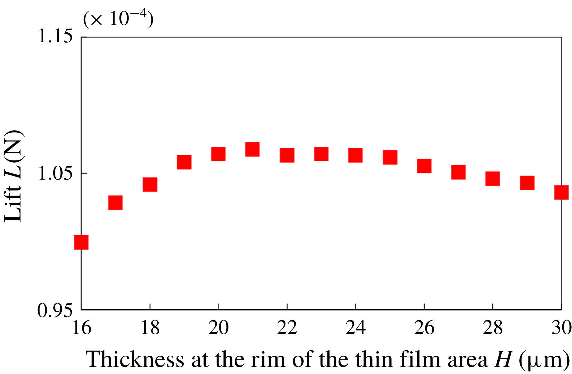
Figure 15. Calculated lift $L$
versus thickness at the rim of the thin-film area
$L$
versus thickness at the rim of the thin-film area $H$
.
$H$
.
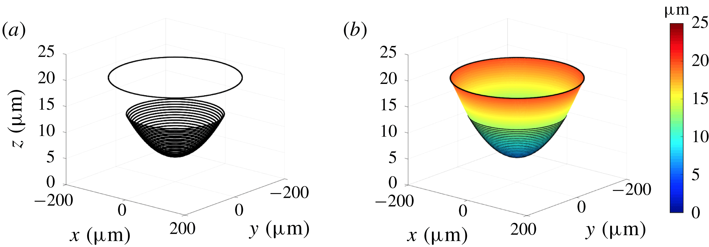
Figure 16. A part of a sphere formed by closed black lines which are substituted for interference fringes (a) before reconstruction and (b) after reconstruction.
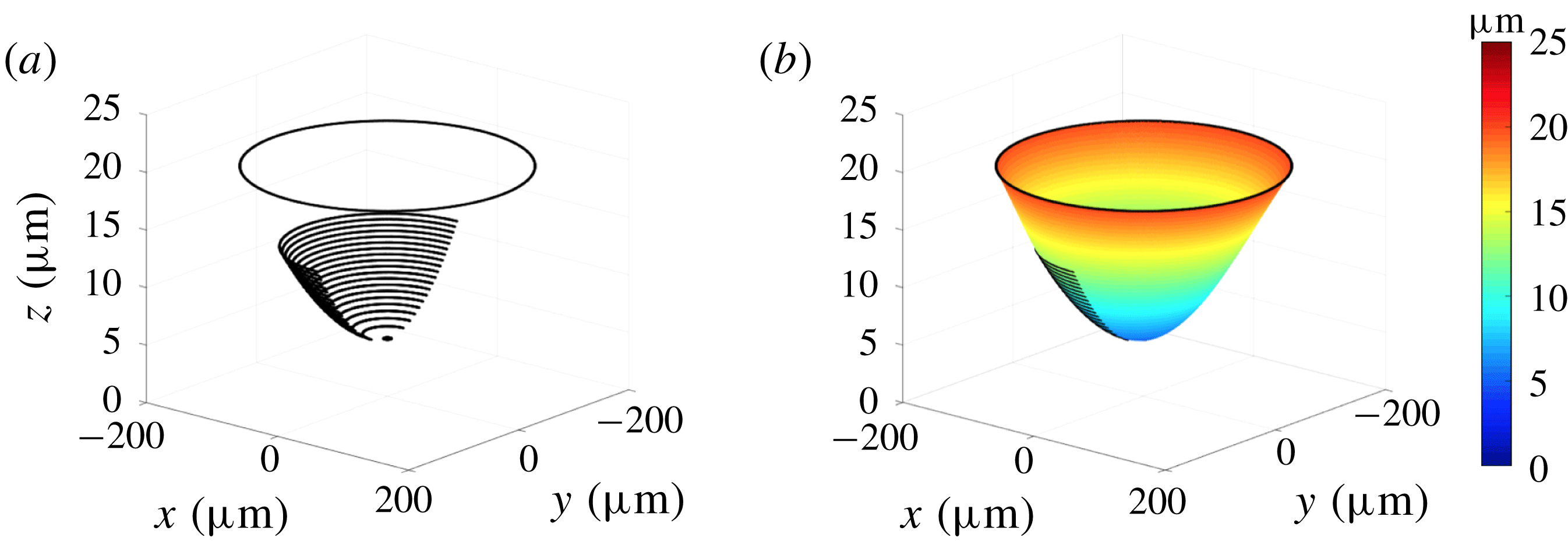
Figure 17. A part of a sphere formed by opened black lines which are substituted for interference fringes (a) before reconstruction and (b) after reconstruction.
Appendix D. Calculation and error estimation for mean curvature
We calculate the mean curvature $\unicode[STIX]{x1D705}$
by using the patch curvature function written in MATLAB. In the function, the least-squares curved surface including the local neighbourhood is calculated at a certain point. By using the eigenvectors and eigenvalues of the Hessian to the curved surface, the mean curvature
$\unicode[STIX]{x1D705}$
by using the patch curvature function written in MATLAB. In the function, the least-squares curved surface including the local neighbourhood is calculated at a certain point. By using the eigenvectors and eigenvalues of the Hessian to the curved surface, the mean curvature $\unicode[STIX]{x1D705}$
is obtained.
$\unicode[STIX]{x1D705}$
is obtained.
We determine the error of the mean curvature $\unicode[STIX]{x1D705}$
as follows. We conduct a smoothing process between fringes to obtain the mean curvature
$\unicode[STIX]{x1D705}$
as follows. We conduct a smoothing process between fringes to obtain the mean curvature $\unicode[STIX]{x1D705}$
. This smoothing process causes the error of the mean curvature
$\unicode[STIX]{x1D705}$
. This smoothing process causes the error of the mean curvature $\unicode[STIX]{x1D705}$
. To investigate the error, we reconstruct a known three-dimensional shape from certain interference fringes, and calculate the mean curvature
$\unicode[STIX]{x1D705}$
. To investigate the error, we reconstruct a known three-dimensional shape from certain interference fringes, and calculate the mean curvature $\unicode[STIX]{x1D705}$
. A part of a sphere of 1 mm in radius is used, where the mean curvature
$\unicode[STIX]{x1D705}$
. A part of a sphere of 1 mm in radius is used, where the mean curvature $\unicode[STIX]{x1D705}$
is
$\unicode[STIX]{x1D705}$
is $10^{3}~\text{m}^{-1}$
. This mean curvature
$10^{3}~\text{m}^{-1}$
. This mean curvature $\unicode[STIX]{x1D705}$
is of the same order as the mean curvature around the minimum thickness of the measured air film. It is inferred that the absolute value of the mean curvature
$\unicode[STIX]{x1D705}$
is of the same order as the mean curvature around the minimum thickness of the measured air film. It is inferred that the absolute value of the mean curvature $\unicode[STIX]{x1D705}$
is large around the minimum thickness, and the error of the mean curvature
$\unicode[STIX]{x1D705}$
is large around the minimum thickness, and the error of the mean curvature $\unicode[STIX]{x1D705}$
is the largest. We set the minimum height of the interference fringes at
$\unicode[STIX]{x1D705}$
is the largest. We set the minimum height of the interference fringes at $5.01~\unicode[STIX]{x03BC}\text{m}$
from the wall, and 19 fringes between
$5.01~\unicode[STIX]{x03BC}\text{m}$
from the wall, and 19 fringes between $5.42$
and
$5.42$
and $13~\unicode[STIX]{x03BC}\text{m}$
at regular intervals. Additionally, the maximum height of the air film (i.e. the rim of the air film) is set at
$13~\unicode[STIX]{x03BC}\text{m}$
at regular intervals. Additionally, the maximum height of the air film (i.e. the rim of the air film) is set at $20~\unicode[STIX]{x03BC}\text{m}$
. We calculate the mean curvature
$20~\unicode[STIX]{x03BC}\text{m}$
. We calculate the mean curvature $\unicode[STIX]{x1D705}$
, when the interference fringes consist of (i) only closed lines which are circles and (ii) closed lines and opened lines which are semicircles. Figures 16(a) and 16(b) show the interference fringes and the reconstructed shape for condition (i), respectively. Figures 17(a) and 17(b) show the interference fringes and the reconstructed shape for condition (ii), respectively. In condition (ii), the fringes at the minimum and maximum height are closed lines, and the others are opened lines. Figures 18(a) and 18(b) show the relative error
$\unicode[STIX]{x1D705}$
, when the interference fringes consist of (i) only closed lines which are circles and (ii) closed lines and opened lines which are semicircles. Figures 16(a) and 16(b) show the interference fringes and the reconstructed shape for condition (i), respectively. Figures 17(a) and 17(b) show the interference fringes and the reconstructed shape for condition (ii), respectively. In condition (ii), the fringes at the minimum and maximum height are closed lines, and the others are opened lines. Figures 18(a) and 18(b) show the relative error $\unicode[STIX]{x1D705}_{err}$
of the mean curvature
$\unicode[STIX]{x1D705}_{err}$
of the mean curvature $\unicode[STIX]{x1D705}$
for conditions (i) and (ii), respectively. Black lines and colour bars indicate the interference fringes and relative error for theoretical mean curvature of the sphere
$\unicode[STIX]{x1D705}$
for conditions (i) and (ii), respectively. Black lines and colour bars indicate the interference fringes and relative error for theoretical mean curvature of the sphere $\unicode[STIX]{x1D705}_{theory}=10^{3}~\text{m}^{-1}$
, respectively. The relative error
$\unicode[STIX]{x1D705}_{theory}=10^{3}~\text{m}^{-1}$
, respectively. The relative error $\unicode[STIX]{x1D705}_{err}$
can be calculated by the equation
$\unicode[STIX]{x1D705}_{err}$
can be calculated by the equation
 $$\begin{eqnarray}\unicode[STIX]{x1D705}_{err}=\frac{\unicode[STIX]{x1D705}-\unicode[STIX]{x1D705}_{theory}}{\unicode[STIX]{x1D705}_{theory}},\end{eqnarray}$$
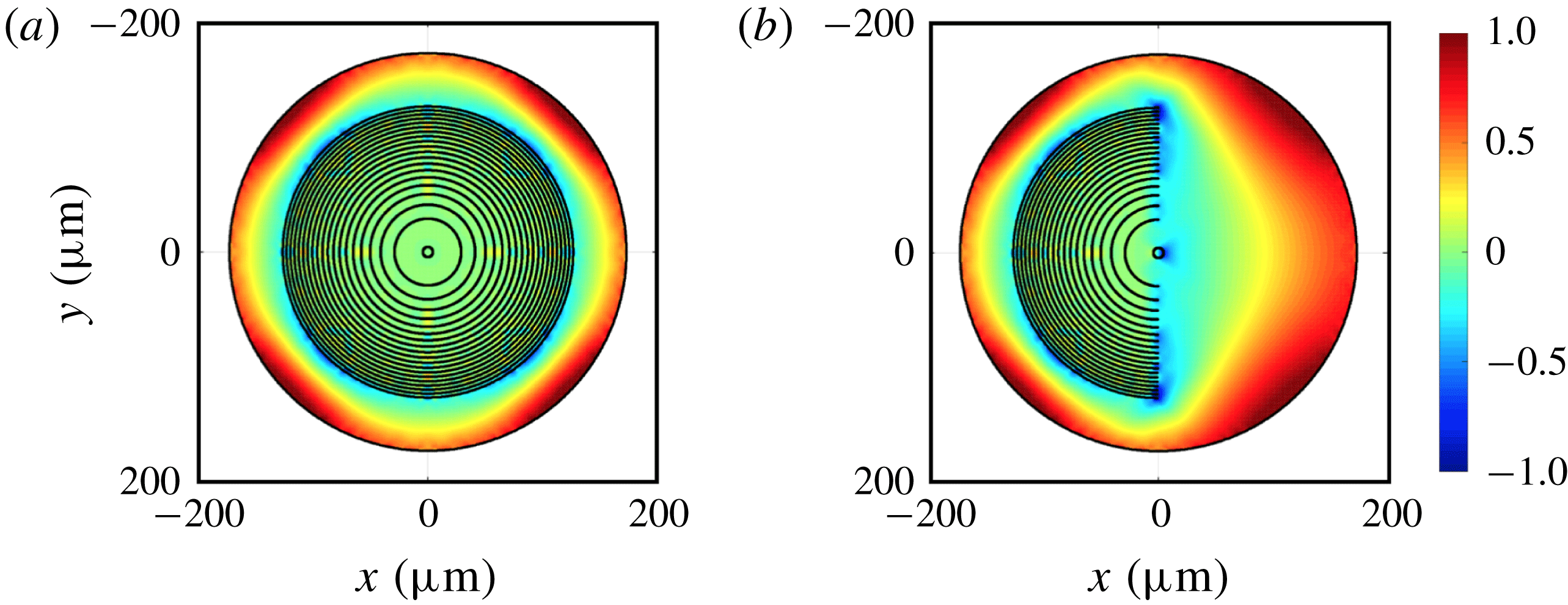
Figure 18. Relative error $\unicode[STIX]{x1D705}_{err}$
of calculated curvature using (a) closed and (b) opened black lines which are substitutes for interference fringes for theoretical mean curvature
$\unicode[STIX]{x1D705}_{err}$
of calculated curvature using (a) closed and (b) opened black lines which are substitutes for interference fringes for theoretical mean curvature $\unicode[STIX]{x1D705}_{theory}=10^{3}~\text{m}^{-1}$
.
$\unicode[STIX]{x1D705}_{theory}=10^{3}~\text{m}^{-1}$
.
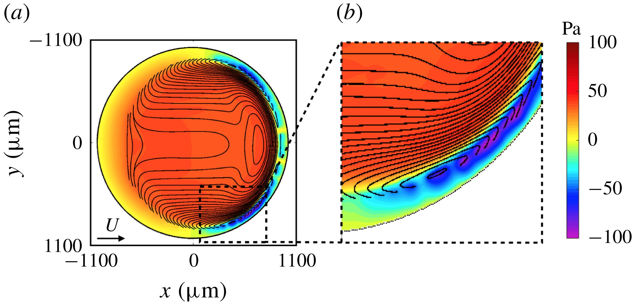
Figure 19. (a) The pressure $p_{s}$
overlaid with obtained interference fringes and (b) enlarged view of (a) around the smallest thickness.
$p_{s}$
overlaid with obtained interference fringes and (b) enlarged view of (a) around the smallest thickness.
where $\unicode[STIX]{x1D705}$
is mean curvature calculated by our method. First, we focus on condition (i) in which the interference fringes consist of only closed lines. As shown in figure 18(a), the error of the mean curvature
$\unicode[STIX]{x1D705}$
is mean curvature calculated by our method. First, we focus on condition (i) in which the interference fringes consist of only closed lines. As shown in figure 18(a), the error of the mean curvature $\unicode[STIX]{x1D705}$
is large around the maximum height of the air film, i.e. the rim of the air film. This is because the area is near to the rim of the air film, in other words, the boundary of calculation. However, when the mean curvature
$\unicode[STIX]{x1D705}$
is large around the maximum height of the air film, i.e. the rim of the air film. This is because the area is near to the rim of the air film, in other words, the boundary of calculation. However, when the mean curvature $\unicode[STIX]{x1D705}$
is calculated in our experiments, interpolation is conducted between the interference fringes and the rim of the air film. Therefore, the significant error of the mean curvature
$\unicode[STIX]{x1D705}$
is calculated in our experiments, interpolation is conducted between the interference fringes and the rim of the air film. Therefore, the significant error of the mean curvature $\unicode[STIX]{x1D705}$
occurs inside the area of the interference fringes in experiments. In this area, the maximum and average of the error of the mean curvature
$\unicode[STIX]{x1D705}$
occurs inside the area of the interference fringes in experiments. In this area, the maximum and average of the error of the mean curvature $\unicode[STIX]{x1D705}$
are about 50 % and 7 %, respectively. Now, we focus on condition (ii). As shown in figure 18(b), the error of the mean curvature
$\unicode[STIX]{x1D705}$
are about 50 % and 7 %, respectively. Now, we focus on condition (ii). As shown in figure 18(b), the error of the mean curvature $\unicode[STIX]{x1D705}$
is large at the ends of the opened lines. The absolute pressure of pressure
$\unicode[STIX]{x1D705}$
is large at the ends of the opened lines. The absolute pressure of pressure $p_{s}$
also increases at the ends of the opened lines in figure 19(b). Thus, the error of the pressure
$p_{s}$
also increases at the ends of the opened lines in figure 19(b). Thus, the error of the pressure $p_{s}$
is due to the increase of the error of the mean curvature
$p_{s}$
is due to the increase of the error of the mean curvature $\unicode[STIX]{x1D705}$
at the ends of the interference fringes. In summary, we find that the smoothing process affects on the error of the mean curvature
$\unicode[STIX]{x1D705}$
at the ends of the interference fringes. In summary, we find that the smoothing process affects on the error of the mean curvature $\unicode[STIX]{x1D705}$
, and the error increases at the open ends of the interference fringes.
$\unicode[STIX]{x1D705}$
, and the error increases at the open ends of the interference fringes.


 Open access