


1. INTRODUCTION
To model the release of a dry-snow slab avalanche, it is essential to understand how failures in snow initiate and develop. Though we have a good conceptual understanding of the key processes involved in slab avalanche release (e.g. Schweizer and others, Reference Schweizer, Reuter, van Herwijnen, Gaume and Greene2016), we still lack a detailed understanding of the first stage, the failure initiation process or in other words the gradual damage process leading to the nucleation of the initial failure. This initial failure can either be caused by an external, rapid, localized load such as a skier or an explosion, or form gradually from local heterogeneities due to slowly changing loading conditions and snow properties. Recent developments in modeling the failure behavior of snow aim to incorporate snow microstructural properties (e.g. Hagenmuller and others, Reference Hagenmuller, Theile and Schneebeli2014; Gaume and others, Reference Gaume, van Herwijnen, Chambon, Birkeland and Schweizer2015). Detailed laboratory studies are needed to constrain and validate microstructural models of damage development and failure initiation in weak snow layers. There is still a lack of understanding with regard to their failure behavior, e.g. the failure envelope (Reiweger and others, Reference Reiweger, Gaume and Schweizer2015a), how damage develops into macroscopic cracks and how the loading rate affects the failure behavior.
Snow is a heterogeneous, highly porous material with strongly rate-dependent material properties. Under tension, at low loading rates, snow fails in ductile manner, while at high loading rates, it exhibits brittle failure (Narita, Reference Narita1983). In displacement-controlled shear experiments, the ductile-to-brittle transition was found to occur at strain rates of 10−4 to 10−3 s−1 (Fukuzawa and Narita, Reference Fukuzawa and Narita1993; Schweizer, Reference Schweizer1998). The rate-dependent behavior was explained by the competition between the damage process and healing due to sintering (de Montmollin, Reference de Montmollin1982; Schweizer, Reference Schweizer1999; Reiweger and others, Reference Reiweger, Schweizer, Dual and Herrmann2009). At slow rates, bond breaking is assumed to be compensated by re-bonding or sintering, whereas at high rates, the damage process dominates and leads to brittle failure. The observed failure behavior in snow was also explained to result from the viscous deformation of the ice matrix (creep) and a viscous-to-brittle transition in ice (Kirchner and others, Reference Kirchner, Michot, Narita and Suzuki2001). Moreover, ice creep can cause relaxation of local load concentrations preventing the initiation of a macroscopic failure, and can be considered as a further mechanism contrasting the damage process. Most probably, a combination of the different mechanisms is involved. We will refer to healing in the rest of the article as the combination of mechanisms compensating the damage process.
Microscopic cracking causes the release of elastic energy in the form of elastic waves, known as acoustic emissions (AE). Recording the AE allows studying the progressive failure in a non-destructive way. It is an established technique for the analysis of the damage process and the detection of failure at an early stage (Grosse and Ohtsu, Reference Grosse and Ohtsu2008). The AE technique is employed for different heterogeneous materials such as concrete (Ohtsu, Reference Ohtsu1996), wood (Bucur, Reference Bucur2006), rocks (Lockner, Reference Lockner1993) or composite materials (Guarino and others, Reference Guarino, Garcimartin and Ciliberto1998) at the laboratory scale as well as at larger scale, e.g. stone cliffs (Amitrano and others, Reference Amitrano, Grasso and Senfaute2005) or glaciers (Faillettaz and others, Reference Faillettaz, Funk and Sornette2011). The failure of disordered materials, such as snow, can also be interpreted as a critical phenomenon with a phase transition from a stable to an unstable phase. The unstable phase is characterized by micro-cracks growing and the correlated damage process culminating in macroscopic failure when a critical density of the damage is reached (Johansen and Sornette, Reference Johansen and Sornette2000).
Previous studies on AE of heterogeneous materials have reported an acceleration of the damage, and of the resulting AE, prior to macroscopic failure and the existence of several AE precursory signals (e.g. Guarino and others, Reference Guarino, Garcimartin and Ciliberto1998). Very similar characteristic features preceding failure were also found for statistical numerical models like fiber bundle and thermal fuse models (e.g. Girard and others, Reference Girard, Amitrano and Weiss2010).
One important parameter is the energy of the AE and its distribution. The energy of the AE usually follows a power-law distribution
 $$P(E)\! \sim \! E^{ - b},$$
where the exponent is usually referred to as the b-value (Guarino and others, Reference Guarino, Garcimartin and Ciliberto1998; Alava and others, Reference Alava, Nukalaz and Zapperi2006). A decrease of the b-value toward failure was reported for laboratory experiments (Lockner, Reference Lockner1993; Guarino and others, Reference Guarino, Garcimartin and Ciliberto1998) as well as for rock cliffs (Amitrano and others, Reference Amitrano, Grasso and Senfaute2005). A decreasing b-value means that the frequency of the large events increases. Furthermore, the decrease has been interpreted as an apparent change in the power-law exponent due to the fact that the energy follows a truncated power-law with diverging cut-off toward failure (e.g. Amitrano and others, Reference Amitrano, Grasso and Senfaute2005). The diverging cut-off theory is supported by the results of numerical simulations (Alava and others, Reference Alava, Nukalaz and Zapperi2006; Girard and others, Reference Girard, Amitrano and Weiss2010; Amitrano, Reference Amitrano2012). For the failure of a hanging glacier, Faillettaz and others (Reference Faillettaz, Funk and Sornette2011) suggested the following b-value evolution: an initial stable state with power-law distribution of AE energy and constant b-value was followed by a phase with energy distribution diverging from the power-law. Close to failure, the power-law behavior recovered with high b-value. A second AE feature indicating an acceleration of the damage process is the increase of the energy release rate, which indicates an increase in size or frequency of the microscopic damage generating the AE. A critical divergence following a power-law of the energy rate  $E(t) \sim [(t_{{\rm \; failure}} - t)/t_{{\rm \; failure}}]^\kappa $ toward the failure point t c was observed for load-controlled laboratory experiments (Guarino and others, Reference Guarino, Garcimartin and Ciliberto1998) and for gravity-driven collapse of a limestone cliff (Amitrano and others, Reference Amitrano, Grasso and Senfaute2005). Johansen and Sornette (Reference Johansen and Sornette2000) observed a power-law increase of the energy rate with log-periodic modulation, which reveal intermittent acceleration and quiescence becoming more closely spaced while approaching failure. In general, a power-law divergence of the energy rate has been observed for load-controlled and constant load (creep) conditions (Guarino and others, Reference Guarino, Garcimartin and Ciliberto1998; Amitrano and others, Reference Amitrano, Grasso and Senfaute2005; Nechad and others, Reference Nechad, Helmstetter, El Guerjouma and Sornette2005; Amitrano and Helmstetter, Reference Amitrano and Helmstetter2006), whereas an exponential increase was reported for displacement-controlled experiments (Guarino and others, Reference Guarino, Garcimartin and Ciliberto1998; Salminen and others, Reference Salminen, Tolvanen and Alava2002). Faillettaz and others (Reference Faillettaz, Funk and Sornette2011) analyzed the inverse waiting time (inverse of time lag between two AE) and observed increasing inverse waiting time toward failure indicating an acceleration of the damage process.
The power-law distribution of the energy is scale invariant, and therefore the b-value does not depend on the absolute value of the AE energy. Similarly, other AE features such as the change in time of the energy rate and the waiting time do not depend on the absolute values of AE amplitude. Hence, these features have the advantage that they are less sensitive to attenuation and material-sensor coupling.
Since the 1970s, several attempts were made to apply the AE technique in snow research. Field studies suggested a connection between increased AE activity and snowpack instability (Sommerfeld, Reference Sommerfeld1977; St. Lawrence and Bradley, Reference St. Lawrence and Bradley1977; Gubler, Reference Gubler1979; Sommerfeld and Gubler, Reference Sommerfeld and Gubler1983; Watters and Swanson, Reference Watters and Swanson1987), whereas other authors reported that quiescent periods may be associated with avalanche activity (Bowles and St. Lawrence, Reference Bowles and St. Lawrence1977; Sommerfeld, Reference Sommerfeld1982). The results of early field studies are partly difficult to interpret due to different experimental set-ups, the different frequency ranges and technical limitations in the signal processing available at that time. St. Lawrence (Reference St. Lawrence1980) developed a relation describing the AE activity as a function of stress and strain for slow deformation of snow. More recently, Scapozza and others (Reference Scapozza, Bucher, Amann, Ammann and Bartelt2004) performed displacement-controlled compression experiments with homogeneous snow samples and observed high-frequency AE (500 kHz) probably due to creep processes in the ice skeleton for strain rates <2 × 10⁻³ s−1 and lower frequency AE (30 Hz) for strain rates >2 × 10⁻³ s−1, which they attributed to cracking. Moreover, Scapozza and others (Reference Scapozza, Bucher, Amann, Ammann and Bartelt2004) reported for low strain rates that the maximum of the AE activity corresponded to the yield point and observed the relation  $\dot N_{{\rm peak}} = C {\dot {\rm \epsilon} } ^\gamma $ between the peak AE rate $\dot N_{{\rm peak}}$ (hits s−1) and the strain rate ${ \dot {\rm \epsilon}} $, with the parameter C being temperature-dependent and γ a constant. Reiweger and others (Reference Reiweger, Mayer, Steiner, Dual and Schweizer2015b) performed load-controlled experiments with layered snow samples including a weak layer (WL) and observed an acceleration of the AE rate before failure as well as a decrease of the b-value very close to complete failure of the sample; they also found this AE behavior in case of partial failure of the sample. Datt and others (Reference Datt, Kapil and Kumar2015) reported for displacement-controlled compression of homogeneous samples a maximum of the b-value at the yield point for low strain rates, and for high strain rates, a decrease of the b-value at brittle fracture.
According to the current theories about the failure of heterogeneous materials (e.g. Johansen and Sornette, Reference Johansen and Sornette2000), failure is the result of the interaction and growth of a multitude of spatially distributed microscopic cracks or damage. It is therefore important to study the damage process on samples of size comparable to the critical size A c for the onset of crack propagation leading to dry snow slab avalanche release (1 dm2 < A c < 1 m2; e.g. Schweizer and others, Reference Schweizer, Kronholm, Jamieson and Birkeland2008); the generated AE may have different signatures from those obtained with smaller samples used in previous studies (Reiweger and others, Reference Reiweger, Mayer, Steiner, Dual and Schweizer2015b). Unlike other heterogeneous materials, snow exhibits strong rate-dependent behavior, which significantly influences also its failure behavior and hence snow strength. The AE response is expected to reveal how damage at the microscale (~1 cm2) develops at different loading rates before complete sample failure.
Given the lack of understanding of how failures in WLs develop, our study aims at monitoring the AE response during snow failure experiments using samples that are large enough to allow for spatial interaction of local failures. We therefore perform load-controlled experiments with large layered snow samples for different loading rates and record the AE generated by the failure process. We use the theory of critical phenomena to analyze the AE response and identify precursory features. In particular, we study the influence of the loading rate on the AE signatures and discuss the implications for understanding the damage process leading to snow failure.
2. METHODS
2.1. Loading apparatus
We developed a new apparatus for fully load-controlled experiments, which allows varying the loading rate and loading angle. The sample size should allow for detecting progressive damage, i.e. failure organization at the microscale, which does not yet lead to complete failure. A schematic representation of the apparatus is shown in Figure 1. The quadratic snow samples had a side length of 50 cm and a height of 10–20 cm. The samples were placed between two rigid metal plates on the top and the bottom parallel to the WL (Fig. 2). The loading force was exerted by the gravitational force of a weight (m = 25–75 kg), which was positioned on a tilting mechanism connected to the top plate by a cable on each side. As the experiment started, the weight was moved horizontally with constant speed by an electrical motor increasing the distance x 1 to the tilting axis, whereas the distance x 2 between the fixation of the cables and the tilting axis was constant. Thus, the loading force exerted on the sample increased linearly with F = m g x 1/x 2. The loading rate could be varied between 4 Pa s−1 and 800 Pa s−1 by modifying the speed of the weight. The load was measured by two force sensors (U9C HBM) at the connection between the top plate and the cables; the maximal possible load was 20 kPa. The loading angle α (angle between top plate and cables) could be varied by changing the horizontal position of the sample on the apparatus. Loading angles between 0° and 45° were possible. The position of the cable fixation to the top plate depended on the loading angle and was adjusted to avoid torque in the WL plane.
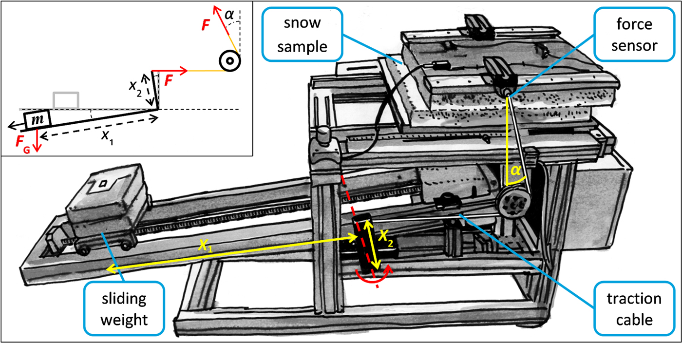
Fig. 1. Schematic representation of the loading apparatus including a snow sample after fracture. The sample failed in the weak layer in the middle. The angle α to the sample simulates the slope angle and can be altered shifting the sample horizontally on the apparatus. The sliding weight exerts the force on the snow sample via the tilting mechanism (red line shows tilting axis) and the traction cable to the metal plate on top of the sample. A motor moves the weight increasing the distance x 1, and hence the load exerted on the sample increases with  $F \!\sim \! x_1/x_2$. The inset shows a schematic representation of the tilting mechanism with the exerted force.
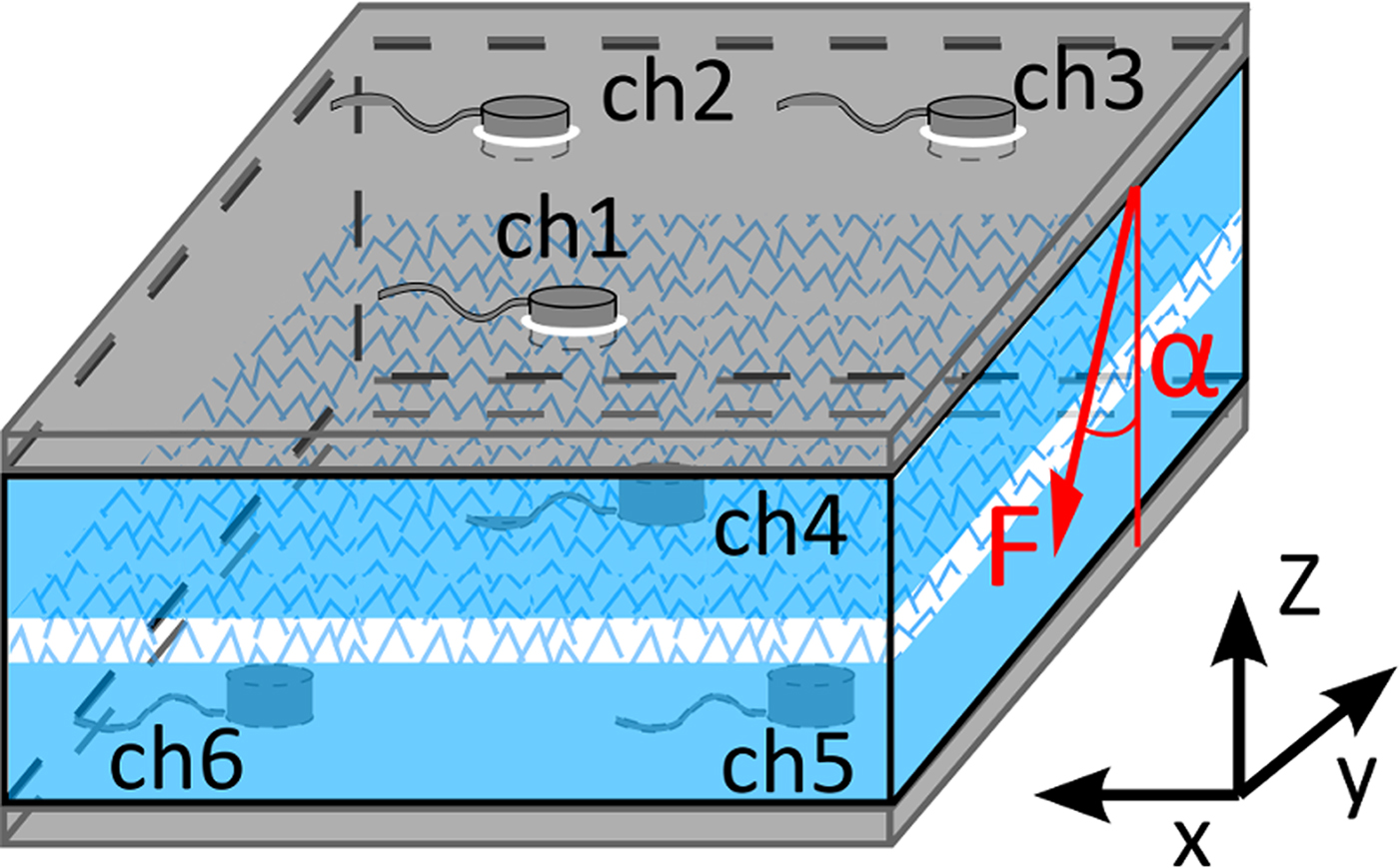
Fig. 2. Schematic representation of a snow sample with the metal plates and the six acoustic sensors (ch1 to ch6). The weak layer plane is parallel to the metal plates. The loading force is applied on the top plate with angle α from the vertical.
2.2. Particle image velocimetry analysis
The displacement field at the side of the samples was determined employing the particle image velocimetry (PIV) technique, which has been previously used to compute the displacement field in snow experiments (e.g. Reiweger and others, Reference Reiweger, Schweizer, Ernst and Dual2010; van Herwijnen, Reference van Herwijnen2013). The displacement field was obtained from a video sequence with 30 fps and 1920 × 1080 pixels resolution (3.6 pixels mm−1) with the Fluere 0.9 PIV software (Lynch and Scarano, Reference Lynch and Scarano2014) comparing the first frame of the video sequence and the consecutive frames. The contrast of the images was enhanced by creating a pattern of dots on the samples. We used a calibration image and second-order image mapping, to correct image misalignment and distortion and convert the displacement field from pixel to millimeter. Vibrations and wobbling of the testing apparatus caused noise in the displacement field, which were corrected by subtracting the displacement of the base plate from the displacement field. A window size of 24 × 24 pixels and a window spacing of four pixels were used for the PIV computation resulting in 450 × 90 measuring points across the sample. The strain in the WL was computed from the difference between the average displacement of two 40-pixels high stripes above and below the WL.
2.3. Recording of the AE
The AE generated during the loading experiments were recorded by six piezoelectric sensors. Three sensors were placed on top of the sample and three sensors at the bottom of the sample (Fig. 2). The sensor arrangement was chosen to allow for AE localization (not presented here). The sensors were inserted into holes going through the metal plates and were frozen to the snow to ensure proper acoustic coupling. We used six wideband piezoelectric acoustic sensors (Mistras WD, 20–1000 kHz). The sampling rate was 1 MHz. The AE were recorded with a system by Physical Acoustics (PCI2 A/D cards), which allowed for real-time waveform acquisition and feature extraction on six channels. A more detailed description of the recording system is found in Reiweger and others (Reference Reiweger, Mayer, Steiner, Dual and Schweizer2015b).
The signals of the acoustic sensors were continuously monitored. Every time a signal exceeded a fixed threshold, a hit with several AE features and the belonging waveform was recorded (Fig. 3). Signal recording ended as soon as the signal did no longer exceed the threshold for a given time. The energy of the hit (given in atto (10−18) Joule: aJ) is the integral of the squared signal amplitude (voltage) over the hit duration divided by a reference resistance (10 kΩ). The waiting time is the time between the end of a hit and the next hit. For a more detailed description and the definition of the AE parameters, the reader is referred to Grosse and Ohtsu (Reference Grosse and Ohtsu2008).
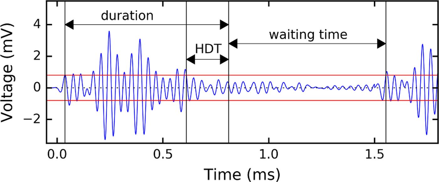
Fig. 3. Exemplary AE signal to illustrate hit detection and feature extraction. The hit starts as the signal exceeds the threshold (red line) and ends when the signal is lower than the threshold for a time longer than the hit definition time (HDT). The waiting time is the distance between two consecutive hits.
Before each experiment, we assessed the acoustic wave attenuation in the snow sample and the losses at the snow–sensor interface with a pencil lead fracture test. This procedure allowed adjusting the signal amplification (20, 40 or 60 dB) and the threshold for each experiment so that they were in the right range. The settings were the same for all channels for a given experiment. Approximate selection in the right range is sufficient since the features we analyzed are robust with respect to changes in the absolute value of the AE signal amplitude. In particular, the b-value, the relative temporal change of the energy rate and the waiting time do not depend on the absolute value of the AE energy.
2.4. Analysis of AE data
The energy of the AE hits is usually distributed according to a power-law relation (Eqn (1)), and the exponent is referred as the b-value. To compute the b-value, we used the python package Powerlaw (Alstott and others, Reference Alstott, Bullmore and Plenz2014) that employs the method described by Clauset and others (Reference Clauset, Shalizi and Newman2009). It allows for a robust fit of power-laws to experimental data. The goodness-of-fit of the b-values was tested comparing the hypothesized power-law distribution with an exponential distribution (Alstott and others, Reference Alstott, Bullmore and Plenz2014). The energy rate was computed with a running time window dividing the sum of the energy by the length of the window. The inverse waiting time was obtained by inverting the mean waiting time, which was as well computed with a running window. The window with time t i included the data points (y i−n, · · · , y i−1, y i), in order to include in the computation just information prior to the time point t i. We used running windows with variable size of n hits for the time evolution of the b-value (n = 250), the inverse waiting time (n = 100 or 300) and the energy rate (n = 100 or 300). For the energy and the waiting time, the separation between two consecutive windows was one hit, whereas for the b-value, it was 20 hits unless otherwise specified. The data of the different channels were always treated separately.
To allow for direct comparison of the energy rate for different loading rates  $\dot \sigma = {\rm d}\sigma /{\rm d}t$, the temporal energy rate dE/dt can be transformed into an energy rate of change with stress dE/dσ = (dE/dt)(dt/dσ) substituting the time t with the stress σ, since the stress increased linearly with time. If an exponential dependence of the temporal energy rate ${\rm d}E/{\rm d}t \sim {\rm e}^{ - \gamma _{\rm t}\; (t_{{\rm failure}} - t)}$ is assumed, the energy rate of change with stress will be also exponential with:
 $$\displaystyle{{{\rm d}E} \over {{\rm d}\sigma}} = \displaystyle{{{\rm d}E} \over {{\rm d}t}}\displaystyle{{{\rm d}t} \over {{\rm d}\sigma}} \sim {\rm e}^{\gamma _{\rm t}\; t}\displaystyle{1 \over {\dot \sigma}} \sim \; {\rm e}^{\gamma _{\rm t}\; \sigma /\dot \sigma} \sim\; {\rm e}^{\gamma _\sigma \; \sigma}, $$
with the relation  $\gamma _{\rm t} = \; \gamma _\sigma \dot \sigma $. In the following, we will refer to the energy rate as the energy rate of change with stress dE/dσ, if not specified otherwise.
2.5. Breeding of synthetic WLs
We produced snow samples including an artificially grown WL of depth hoar crystals following the method described by Fukuzawa and Narita (Reference Fukuzawa and Narita1993). A snow sample was prepared with an area of 50 cm × 120 cm and height of 12–15 cm consisting of three layers of different density (Fig. 4). The 5 cm thick base layer was produced by sieving natural snow (rounded grains) through a fine mesh (2 mm) directly onto the bottom metal plate used for the shear apparatus. The middle layer, the subsequent WL, was produced by sieving machine-made nature-identical new snow (Schleef and others, Reference Schleef, Jaggi, Löwe and Schneebeli2014) through a coarser mesh (8 mm) onto the bottom layer. The thickness of this layer was ~15 mm. The top layer, ~6 cm in thickness, was produced separately using the same method as for the base layer. After 2–3 d of sintering (at −20 °C), the top layer was placed on the low-density middle layer. Then, the layered sample was subjected to a temperature gradient of 1–1.5 K cm−1 for 7 d inducing snow metamorphism. As a result, the snow of the less dense middle layer was transformed to depth hoar. The depth hoar structure is anisotropic, coarse and loosely bonded, and therefore particularly fragile under shear loading (Reiweger and Schweizer, Reference Reiweger and Schweizer2013). The snow of the base and top layer was transformed as well, but due to its higher density, the metamorphism was less pronounced. From every breading sample, we obtained two samples for the loading experiments with a quadratic area of 50 cm × 50 cm each. The remaining section in the middle was used for the snow characterization (Table 1). Grain size, grain type, hand hardness index and density were characterized as described in Fierz and others (Reference Fierz2009). Three snow micro-penetrometer resistance profiles were recorded (Schneebeli and Johnson, Reference Schneebeli and Johnson1998) for each sample. In addition, we characterized the microstructure by x-ray computer tomography (Schneebeli and Sokratov, Reference Schneebeli and Sokratov2004). For each layer, a section with a volume of 15 mm × 15 mm × 4.5 mm was scanned and used to derive the snow properties.
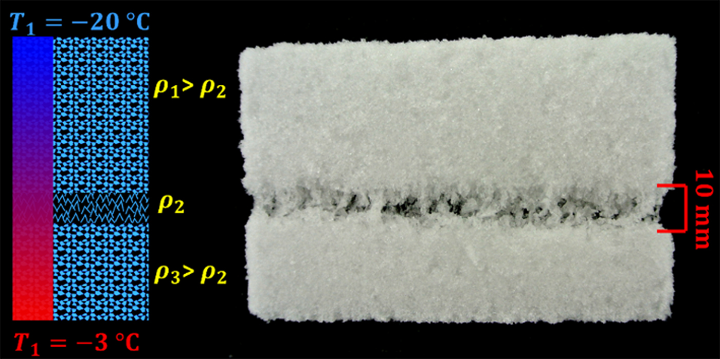
Fig. 4. Layered sample including a weak layer: schematically (left), thin section (right). The coarse depth hoar weak layer in the middle is well visible.
Table 1. Snow properties of top layer (slab), weak layer and bottom layer (base). We report the mean and the range, except for hand hardness index we provide the median, and for grain shape the most frequent shape.

3. RESULTS
We performed loading experiments with different loading rates (400, 168 and 32 Pa s−1). In the first section of the results, we describe our findings on the mechanical deformation. In the second section, we present the typical AE features observed before failure. Finally, we report the influence of the loading rate on the AE response and discuss some cases of samples that did not fail.
Table 2 shows a summary of the loading experiments. Most samples loaded at the lowest loading rate (32 Pa s−1) did not fail. Only sample LDL04B failed during the second loading cycle. The first loading cycle was stopped at 13.8 kPa without reaching the failure point. The loading experiments were performed with different loading angles (α = 0°, 15° and 35°). We did not observe any significant dependence of the AE signature on the loading angle. Therefore, we do not take into account the loading angle in the following analysis.
Table 2. Summary of the test conditions and results for the 18 samples used for this study
The applied load induced a progressive deformation of the samples. An exemplary displacement field obtained with PIV is shown in Figure 5. The deformation was concentrated in the zone between 60 and 50 mm height corresponding to the WL where the failure eventually occurred. A concentration of the deformation in the WL was observed for all samples. At failure, a crack was formed along the WL, and consequently led to the collapse of the WL. The propagation of the crack could not be observed. In Figure 6a, we exemplarily compare the stress–strain relations of three experiments (samples LDL07A, LDL12B and LDL04B) with different loading rates at the same loading angle α = 35°. For the experiments with the high loading rates (168 and 400 Pa s−1), we observed brittle fracture with very low strain prior to failure. For the slowest experiment (32 Pa s−1), we observed much larger strain, and at 13.8 kPa, the experiment was stopped without reaching complete failure. Figure 6b shows the strain rate as a function of increasing stress. We used a Kalman filter (Kalman, Reference Kalman1960) to extract the strain rate from the noisy strain data. The strain rate considerably varied. To show the general trend, we fitted a linear function to the strain data (Fig. 6b, dotted line). The strain rate increased with increasing load for all loading rates and reached ~2 × 10⁻⁴ s−1 for a loading rate of 400 Pa s−1 and 0.9 × 10⁻⁵ s−1 for 168 Pa s−1 (strength 8.1 and 8.3 kPa, respectively). For the slow loading rate of 32 Pa s−1, the strain rate reached ~4.5 × 10⁻⁴ s−1.
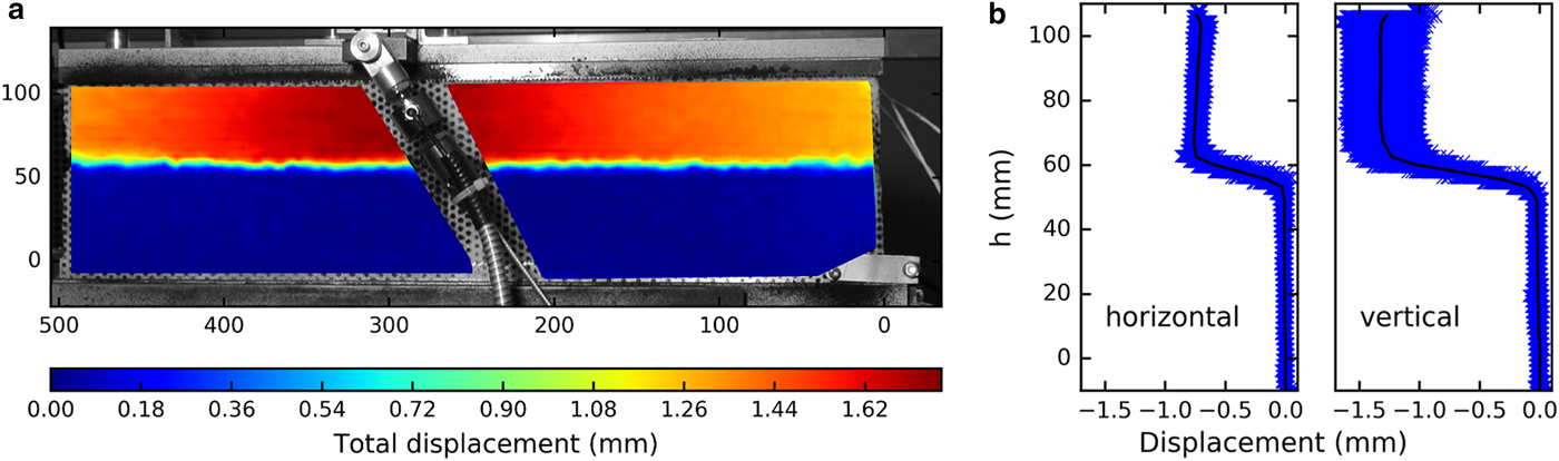
Fig. 5. (a) Two-dimensional map of the total displacement relative to the bottom plate immediately before failure. The x- and y-axis show the dimension of the sample in mm. (b) Vertical and horizontal displacement at different heights. The scatterplot in blue shows the values for each evaluated point. The black lines indicate the mean at each height h. Sample LDL04B with loading angle α = 35°.
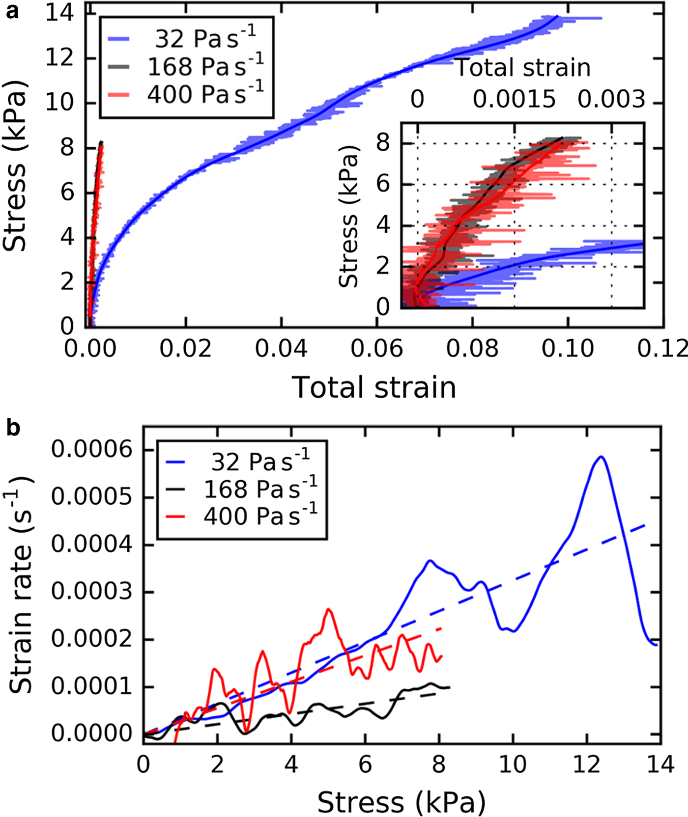
Fig. 6. (a) Stress–strain relation of weak layer for three experiments with different loading rates. The inset shows the stress for very low strain (below 0.0035). (b) Strain rate vs stress for the same three experiments. The solids lines in (a) and (b) were obtained from the noisy data with a Kalman filter; the dashed line in (b) is a linear fit of the strain rate. The loading angle was α = 35° for all three samples (LDL04B_load01, LDL12B and LDL07A).
3.1. AE signatures before failure
We will describe the failure process and the typically observed AE signatures using the sample LDL07A (α = 35°, stress rate = 400 Pa s−1) as an illustrative example, in particular focusing on the features in the AE signal characteristic for the time preceding complete failure of the sample.
3.1.1. Energy distribution and b-value
The probability density of the energy E of the recorded AE for the sample LDL07A and its evolution in time were analyzed (Fig. 7). The goodness-of-fit of the power-law distribution was tested by comparing it to an exponential distribution. The power-law fit was better than the exponential fit regardless whether all events up to fracture or only events in a given time window were considered. However, the corresponding complementary cumulative distributions exhibited a significant curvature (Fig. 7b). The b-value for all the events up to fracture was 1.55 ± 0.2 (channel 2). Figure 7 shows (a) the evolution of the b-value toward failure computed using a running window of n = 250 hits and a minimum value for the fit of 600 aJ, and (b) the complementary cumulative distribution of event energy for eight different running windows with the corresponding power-law fits for channel 2. The initial b-value for channel 2 was ~2.5 and decreased continuously to 1.4 at failure. The decrease of the b-value was observed for each channel with similar initial and final b-values for all channels except for channel 1, which had a poor sensitivity and recorded only few hits during the last 2.5 s of the experiment.
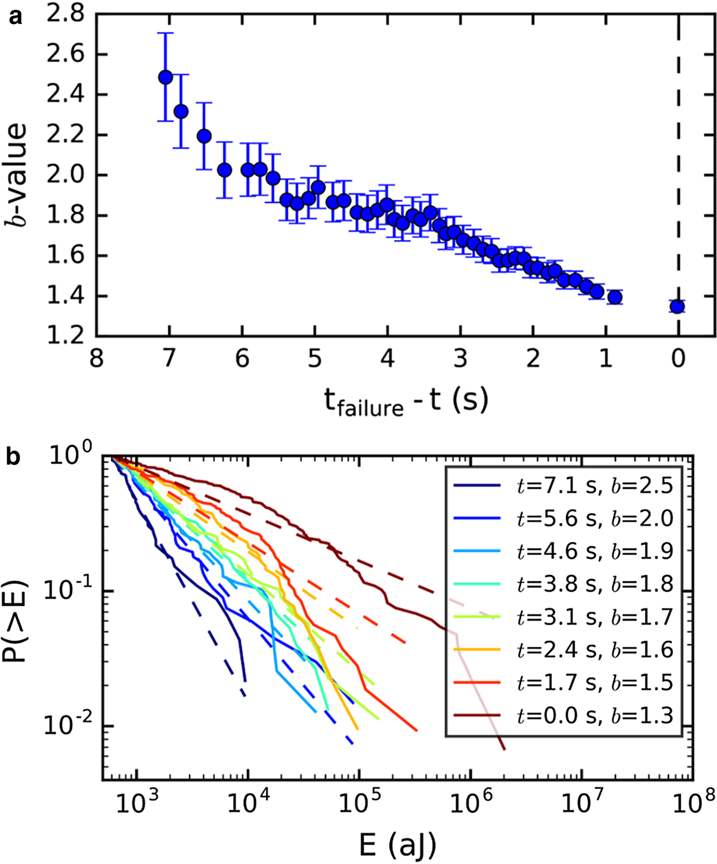
Fig. 7. (a) Evolution of b-value toward failure for sample LDL07A, ch2. Running window size n = 250 hits. The error bars indicate the std dev. (b) Complementary cumulative distribution of energy E for eight different windows with corresponding power-law fits (dashed lines). The time t in the legend indicates the time before complete failure.
3.1.2. Energy rate
The AE energy rate is an indicator of the amount of new damage created in the sample, since elastic energy is released in the form of acoustic waves whenever a micro-crack forms or grows. The energy rate before failure for sample LDL07A computed with a moving window n = 100 hits is shown in Figure 8. The AE energy rate increased exponentially toward failure. The coefficient γ σ was computed with a linear regression of the logarithmic scaled energy rate (red line in Fig. 8). The energy rate at failure varied by almost two orders of magnitude between the different channels, since the magnitude of the measured AE signal depends on sensor–snow coupling and attenuation within snow. However, the increase is expected to be independent of the absolute value of the AE signal. Nonetheless, we observed some variation between channels of the exponential coefficient γ σ and the range at which the energy rate increased exponentially. The mean value of all six channels was γ σ = 1.4 ± 0.5 × 10⁻³ Pa−1. The many orders of magnitudes higher energy rate recorded at and after failure was produced by the collapse of the WL and by friction during the sliding or the upper slab after failure.
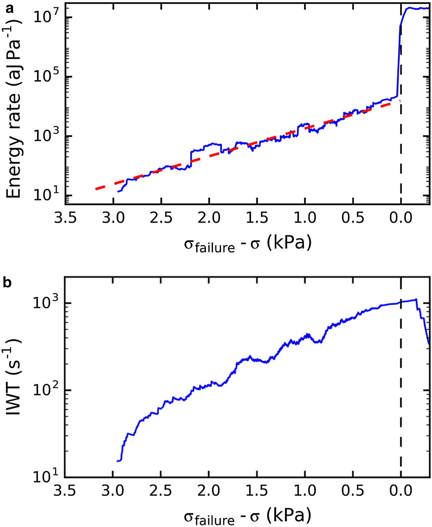
Fig. 8. (a) Energy rate evolution with increasing load for sample LDL07A (ch2; n = 100 hits). The red dashed line represents a linear fit of the logarithmically scaled energy rate, which increased exponentially before failure. (b) Evolution with increasing load of the inverse mean waiting time (IWT) for sample LDL07A (ch2) with running window size n = 100 hits.
3.1.3. Inverse waiting time
The waiting time is defined as the time between the end of an AE hit and the start of the next, and therefore, the inverse waiting time is the hit mean frequency or frequency of the AE activity. The time evolution of the inverse mean waiting time for the sample LDL07A channel 2 is shown in Figure 8b. We observed an exponential increase of the inverse waiting time toward failure. The exponential increase was observed for all channels, but had different magnitudes. The increase of the inverse waiting time indicated an acceleration of the damage frequency, since the time between two hits decreased.
3.2. Loading rate dependence of AE signatures
Given that the deformation and failure behavior depends on loading rate (see above), we expected also the AE response to depend on loading rate. We computed the time evolution of the b-value for samples, which were loaded with three different loading rates (32, 168 and 400 Pa s−1). Figure 9 shows examples of the evolution of the b-value for each loading rate (samples: LDL07A, LDL12B and LDL04B_load02). For all three rates, the power-law distribution provided the better fit for all windows. For the low loading rates, the decrease of the b-value was less pronounced. The b-value for the only sample with the lowest loading rate which failed (LDL04B_load02) was almost constant considering the entire loading period and the b-value at failure was higher. However, a modest decrease of the b-value was observed shortly before failure (Fig. 9). To allow for comparison of the results, we performed a linear regression with b = a (t failure − t/t failure) + c (dashed line in Fig. 9). We performed the fit on b-value evolution of several experiments with different loading rates (five samples and 19 channels for 400 Pa s−1, and four samples and 18 channels for 168 Pa s−1). The channels and samples for which too few AE hits (<800) were available were not considered for the evaluation. The results of the fits are summarized as boxplots in Figure 10. The median value of the slope a was lower for the lower loading rate (a = 1.4 for 400 Pa s−1 and a = 0.5 for 168 Pa s−1), whereas the value of the fitting line at t = t failure was higher for the slower loading rate (c = 1.3 for 400 Pa s−1 and c = 1.6 for 168 Pa s−1). The mean coefficient of determination R 2 was 0.45 for 400 Pa s−1 and 0.25 for 168 Pa s−1. The P-value was below 0.002 for all linear regressions. For some samples, the slope was almost zero or even negative. However, we observed a decrease of the b-value shortly before failure at least in one channel for every sample.
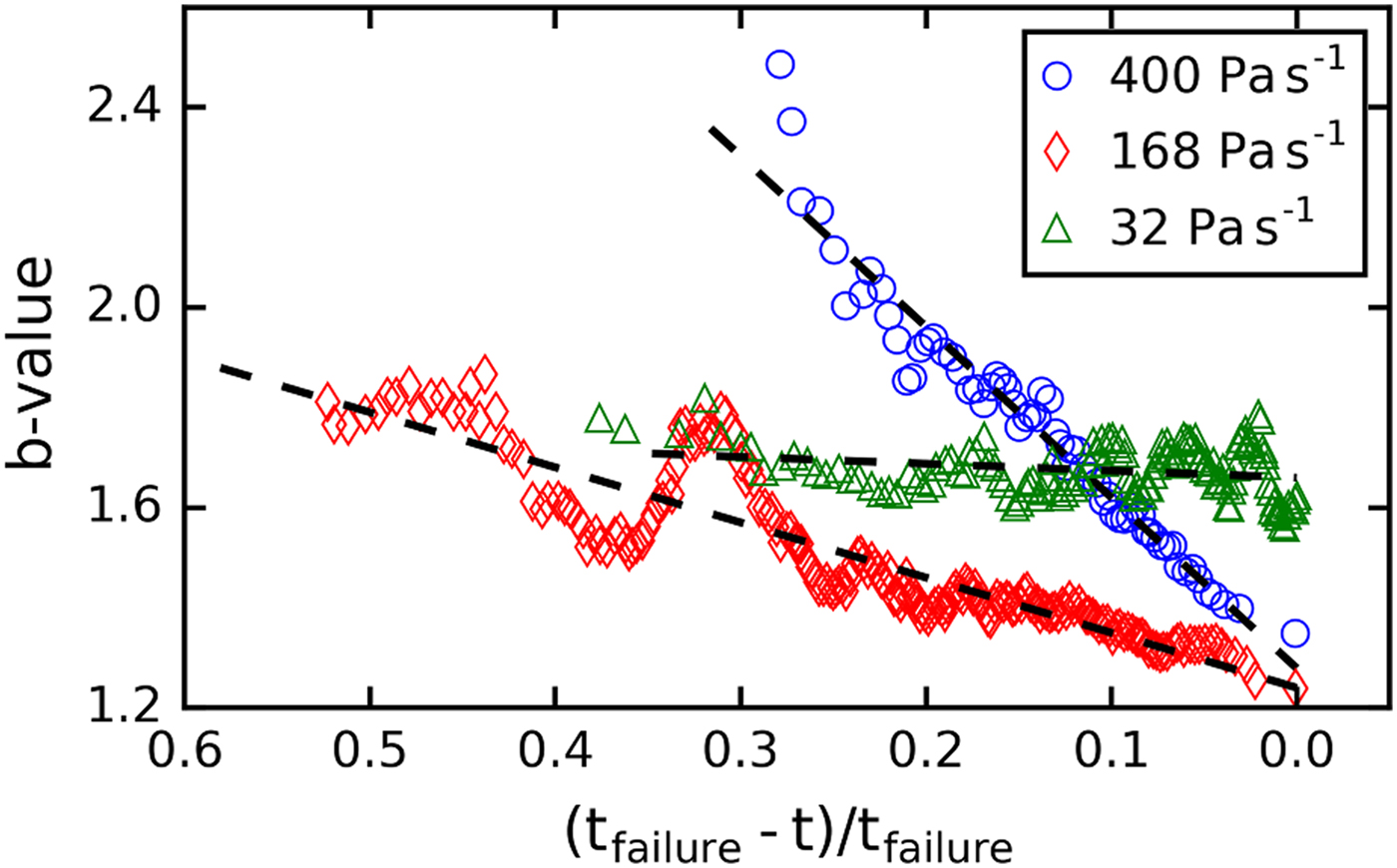
Fig. 9. Evolution of b-value before complete failure for different loading rates (400, 168 and 32 Pa s−1). The dashed lines represent a linear regression. Samples shown: LDL07A, LDL12B and LDL04B_load02, window size n = 250.
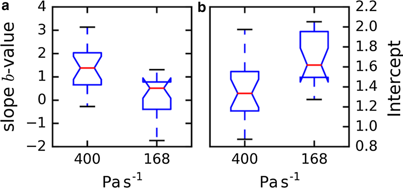
Fig. 10. Boxplots summarizing the linear regression to the b-value time evolution of several samples for two different loading rates (168 Pa s−1, N = 18; 400 Pa s−1, N = 19). (a) The slope of the b-value evolution with time. (b) b-value at failure obtained from the intercept of the linear fit at the failure point.
The absolute value of the energy rate per unit time dE/dt was higher for the experiments at higher loading rates. This finding is not surprising since with a faster increase of the load, a higher damage rate and consequently a higher AE energy rate is expected. To allow for direct comparison, we used the energy rate per unit stress dE/dσ. Figure 11 shows an example of the temporal evolution of the energy rate dE/dσ for the three loading rates. The energy rate increased exponentially before complete failure for all loading rates. However, the range over which the exponential growth was observed varied substantially between the samples and channels. The exponential coefficient γ σ and the energy rate at failure were obtained with a linear regression of the logarithm of the energy rate for several samples. The channels and samples for which too few AE hits (<800) were available were not considered for the evaluation. The time range for the fit was chosen manually for each channel. Figure 12 shows the exponential coefficient γ σ and the energy rate at failure for the experiments with the two loading rates 400 and 168 Pa s−1. The mean value of γ σ was almost the same for both loading rates (1 × 10⁻³ Pa−1 for 400 Pa s−1 and 0.9 × 10⁻³ Pa−1 for 168 Pa s−1). The mean exponential coefficient for the single slow experiment that completely fractured was γ σ = 0.35 × 10⁻³ Pa−1 (LDL04B_load02, mean over five channels). This value was one-third of the value observed for the samples with brittle fracture. The energy rate at failure was similar at the two faster loading rates (Fig. 12b) and for the single slow experiment that failed (dE/dσ(σfailure) = 104.7±0.5 aJ Pa−1). However, the absolute value of the energy rate cannot easily be compared since the measured energy values depend strongly on the sensor–snow coupling and attenuation within snow (1 dB cm−1; Capelli and others, Reference Capelli, Kapil, Reiweger, Or and Schweizer2016) and the absolute values varied considerably (Fig. 12b).
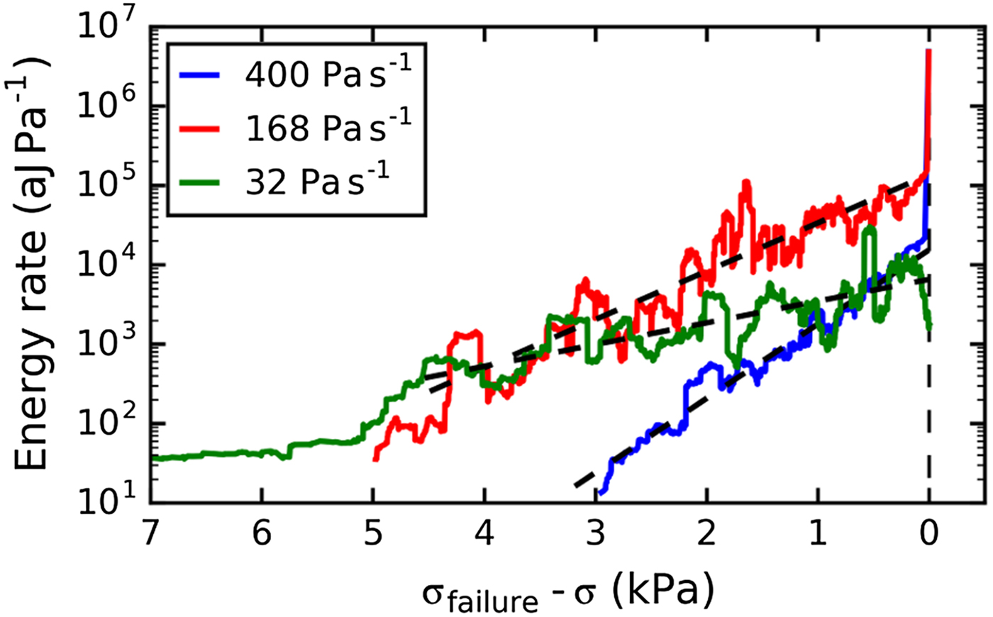
Fig. 11. Evolution of the energy rate with increasing load for three different loading rates. Samples shown: LDL07A, LDL12B and LDL04B_load02, window size n = 100.
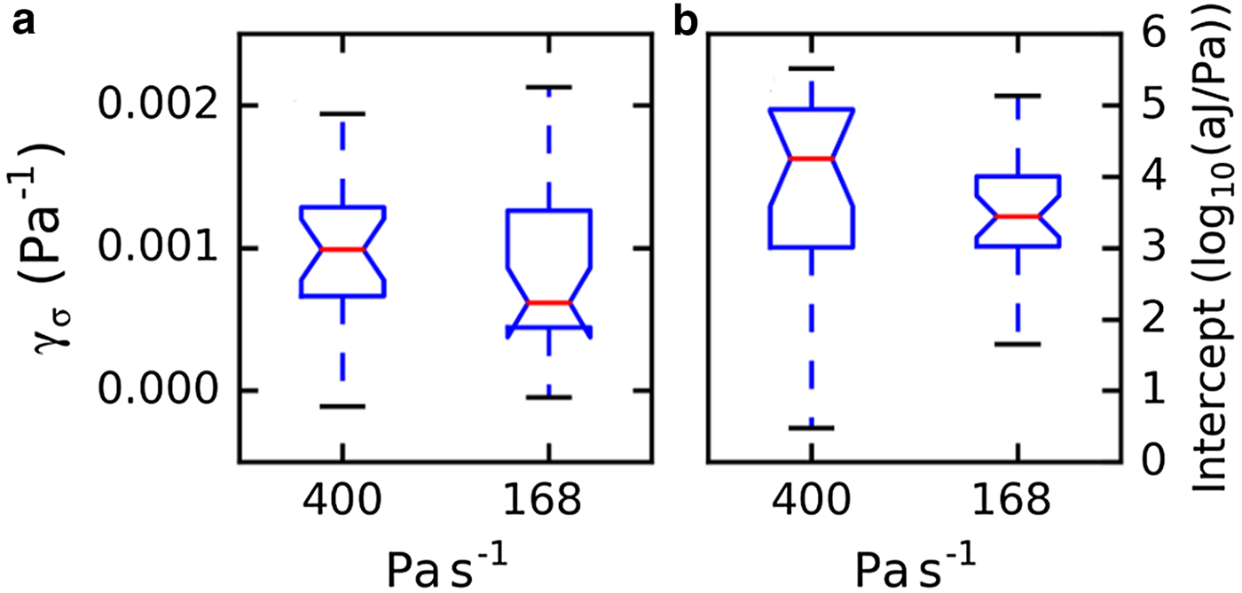
Fig. 12. Boxplots summarizing the temporal evolution of the energy rate for several samples and for two different loading rates (168 Pa s−1, N = 18; 400 Pa s−1, N = 19). (a) Exponential coefficient γ σ. (b) Energy rate at failure (logarithmic scale) obtained from the intercept of the linear fit at the failure point.
The magnitude of the inverse waiting time was much lower for the slower experiments, whereas the evolution before failure was similar for all three loading rates (Fig. 13). The waiting time increased exponentially before failure for all three loading rates.
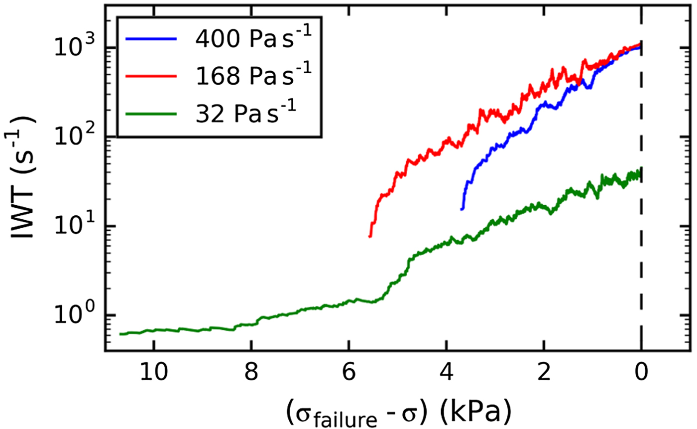
Fig. 13. Evolution of the inverse waiting time with increasing load for different loading rates. Samples shown: LDL07A, LDL12B and LDL04B_load02, window size n = 100.
3.3. AE signatures in the absence of complete failure
In the following, we present two examples of loading experiments without complete failure of the sample and analyze the observed AE features. Sample LDL04B was loaded with 32 Pa s−1 up to 13.8 kPa without fracturing. Figure 14 shows the time evolution of b-value, inverse waiting time and energy rate. For all windows, the power-law distribution provided the better fit, and the b-value did not change much over the entire duration of the experiment but varied. Similarly, the inverse waiting time and the energy rate did not increase exponentially as observed for the samples that failed, but varied with increasing amplitude in time. The constant b-value as well as the lack of exponential increase of energy rate and inverse waiting time suggest that the damage process was stable, i.e. did not change over the entire duration of loading. However, the variations indicate that the damage process was not continuous but consisted of a series of bursts, the size of the bursts increasing with increasing load.
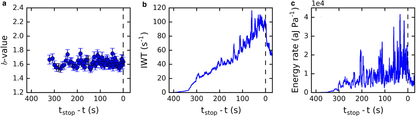
Fig. 14. AE features for the sample LDL04B (ch2), which was loaded with 32 Pa s−1 and did not fracture. Evolution with time for (a) b-value (running window size n = 300 hits, window separation 200 hits), (b) inverse waiting time (IWT) (n = 300 hits), (c) energy rate (n = 200 hits). The error bars indicate the std dev.
The second example of a loading experiment without complete failure is sample LDL07B, which was loaded at a rate of 168 Pa s−1. In addition to the previously described decrease of b-value and increase of energy rate and waiting time over the entire duration of the experiment, we observed a spike in the inverse waiting time, and energy rate with a simultaneous rapid decrease of the b-value at 28.2 s before reaching the maximum load (Fig. 15, dotted red line). All parameters indicated an acceleration of the damage process over a short time without observing fracture of the whole sample. Moreover, the magnitude of the observed change in the AE features varied strongly from channel to channel. It was pronounced for ch1, ch2 and ch5, whereas for the other channels (ch3, ch4 and ch6) was barely visible. We assume that the acceleration of the AE activity was caused by a major local failure that did not spread through the entire sample (partial failure). The AE response was, therefore, not equally present in the overall signal of the different channels, since the attenuation was higher for the sensors further away from the source.
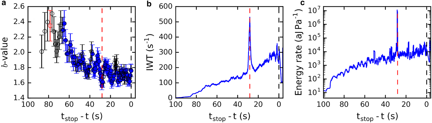
Fig. 15. Example of AE features in case of a local failure that did not lead to failure of the entire sample (LDL07B ch1; 168 Pa s−1). The local failure is marked by the red dashed vertical line at 28.2 s. The sample reached the maximum load of 20 kPa without failing. Evolution with time for (a) b-value (running window size n = 250 hits, window separation 100 hits), (b) inverse waiting time (IWT) (n = 300 hits), (c) energy rate (n = 100 hits). In the b-value evolution plot, the blue dots indicate that the power-law distribution provided the better fit than an exponential distribution; and vice versa for the red indicating that the exponential distribution yielded a better fit. The cases shown with open circles are those for which the goodness-of-fit was low and the model was not appropriate with 90% confidence (P-value >0.1). The error bars indicate the std dev.
4. DISCUSSION
4.1. AE signatures prior to failure
The deformation and, consequently, the damage were concentrated in the WL where eventually the crack formed so that the sample failed completely. Therefore, we assume that the majority of the recorded AE were generated in the WL and carry information about the damage process. We identified several features in the AE signatures for the time preceding failure that seem indicative of the ongoing damage process. The energy rate and the mean inverse waiting time increased before failure implying an increase of the size and frequency of the AE events (Figs 8, 9a). We interpret the increase of size and frequency of the AE events as an acceleration of the damage process with increased size and frequency of damage and/or micro-cracks generating the AE.
The AE energy was power-law distributed indicating a scale invariance of the AE and the b-value decreased approaching failure (Fig. 7). The complementary cumulative distributions exhibited a significant curvature indicating a deviation from a power-law (Fig. 7), which may have multiple origins. According to Weiss (Reference Weiss1997), the curvature may be due to the high attenuation of the acoustic waves, which has been shown for snow (Capelli and others, Reference Capelli, Kapil, Reiweger, Or and Schweizer2016). An alternative reason may be that the AE energy distribution follows a truncated power-law with exponential cut-off, which is given by the finite size of the system. The observed decrease of the b-value could be due to a diverging cut-off approaching failure, which would result in an apparent b-value decrease (Amitrano and others, Reference Amitrano, Grasso and Senfaute2005; Alava and others, Reference Alava, Nukalaz and Zapperi2006; Girard and others, Reference Girard, Amitrano and Weiss2010). The goodness-of-fit of a truncated power-law will almost always be better compared with a simple power-law, since a function with two parameters can adapt better to the empirical data (Alstott and others, Reference Alstott, Bullmore and Plenz2014). However, the use of a truncated power-law has two main disadvantages: (1) the additional parameter increases the complexity of the analysis, and (2) the identification of the exponential tail can be difficult due to the limited number of events used for the fit (Amitrano, Reference Amitrano2012). The second problem could be mitigated by increasing the window size, causing, however, a decrease of the temporal resolution. Therefore, we used a simple power-law fit for the evaluations presented in this work, since the apparent decrease of the b-value provides a valid precursory pattern (Amitrano, Reference Amitrano2012).
The decrease of the b-value corresponds to a change in the event distribution statistics and indicates that the portion of events with high energy increases before failure. A similar continuous decrease of the b-value was observed for the collapse of a rock cliff (Amitrano and others, Reference Amitrano, Grasso and Senfaute2005) and in numerical simulations of failure behavior (e.g. Girard and others, Reference Girard, Amitrano and Weiss2010; Pradhan and others, Reference Pradhan, Hansen and Chakrabarti2010; Amitrano, Reference Amitrano2012). A decrease of the b-value is often attributed to a transition from homogeneously distributed uncorrelated damage producing mostly small AE to larger correlated events, or in other words, to local stress concentrations causing localized damage (Johansen and Sornette, Reference Johansen and Sornette2000; Girard and others, Reference Girard, Amitrano and Weiss2010). Although we do not have any direct proof of a change to localized and correlated damage before failure of snow, by analogy to other materials and numerical models, we assume that this change is likely taking place since we observed a feature, namely the decrease of b-value, which is often related to this transition from uncorrelated to localized damage leading to failure (Lockner, Reference Lockner1993; Guarino and others, Reference Guarino, Garcimartin and Ciliberto1998; Girard and others, Reference Girard, Amitrano and Weiss2010).
For snow, Reiweger and others (Reference Reiweger, Mayer, Steiner, Dual and Schweizer2015b) observed a drop in the b-value shortly before brittle fracture, whereas we observed a progressive decrease of the b-value. The experimental setup and the analysis method employed by Reiweger and others (Reference Reiweger, Mayer, Steiner, Dual and Schweizer2015b) were similar to those in our study, however, with the difference that our sample size was ~10 times larger (basal area: 200 cm2 vs 2500 cm2). A decrease of the b-value coincident with brittle failure was also observed by Datt and others (Reference Datt, Kapil and Kumar2015) for samples of even smaller size (~35 cm2). Therefore, we suggest that the observed difference in timing of the b-value decrease may be due to size effects. For small samples, the development of a major damage zone may quickly lead to complete failure of the sample. On the other hand, for large samples, the load may be redistributed allowing the progressive formation of several damage zones up to a critical point when finally the whole sample fails. This interpretation is supported by the observation of partial failures (Fig. 15). As in the case of the small samples, for the partial failures, the acceleration occurred on a short timescale compared with the duration of the experiment.
According to the theory of critical phenomena, the energy rate should diverge approaching failure following a power-law as was observed for load-controlled failure (Guarino and others, Reference Guarino, Garcimartin and Ciliberto1998; Amitrano and others, Reference Amitrano, Grasso and Senfaute2005) and for numerical simulations (e.g. Girard and others, Reference Girard, Amitrano and Weiss2010). Similarly, a divergence of the inverse waiting time was observed by Faillettaz and others (Reference Faillettaz, Funk and Sornette2011). In contrast, we observed an exponential increase of the energy rate and inverse waiting time without divergence at failure. In fact, an exponential increase was previously reported for displacement-controlled experiments (Guarino and others, Reference Guarino, Garcimartin and Ciliberto1998; Salminen and others, Reference Salminen, Tolvanen and Alava2002). If the number of AE events per unit time is too high, the signals of distinct AE will be superimposed and measured as a single hit. This can explain the absence of the divergence in the waiting time. However, this is not true for the energy rate, since the much higher energy rate measured after failure shows that the maximum measurable energy rate was not reached before failure (see Fig. 8a). A possible explanation of our findings is that sintering (healing) counteracts the damage and hence inhibits the divergence toward failure.
4.2. Rate-dependent behavior of snow and resulting AE features
As expected, the deformation and failure behavior strongly depended on the loading rate. The strain at equal stress was much higher for the lowest loading rate and the majority of samples did not fail. The strain rate increased with increasing load for all loading rates. For example, as shown in Figure 6, the strain rate for the experiments with the lowest loading rate increased to 4.5 × 10⁻⁴ s−1 at a load of 13 kPa, a value even higher than measured for the experiment with the highest loading rate. This finding suggests that the deformational behavior of the sample significantly changed with increasing load, presumably as consequence of damage accumulation and subsequent change in the snow microstructure.
Our results are in accordance with the previous experimental observations on the failure behavior as a function of loading rate (Narita, Reference Narita1983; Schweizer, Reference Schweizer1998; Reiweger and Schweizer, Reference Reiweger and Schweizer2013). Schweizer and others (Reference Schweizer, Jamieson and Schneebeli2003) reported a transition from ductile to brittle behavior at ~10−3 to 10−4 s−1 for displacement-controlled shear experiments. However, we observed for the load-controlled experiments comparatively high strain rates at slow loading rates. Still, in our experiments, we did not observe brittle fracture due to experimental constraints, i.e. the maximum load was limited. These findings suggest that depending on the type of load, the strain rate alone is not sufficient to control the ductile-to-brittle transition, and that a more complex model is necessary to describe the snow failure behavior. As we observed that even at slow loading rates with ongoing damage process in the WL high strain rates may develop, we may argue that in combination with the inherent inhomogeneity of the snowpack, high stress rates may develop eventually leading to brittle fracture – and avalanche release.
The rate-dependent failure behavior of snow was also reflected in the AE emission signatures. The b-value decrease toward failure was lower for the lower loading rates with almost constant b-value for the lowest rate in the ductile range. The observed differences in the b-value evolution are in accordance with the observed difference between the ductile and brittle failure behavior and allow hypothesizing on the micromechanical origin of that difference in the failure behavior. The b-value decrease observed for the high loading rates can be interpreted as transition from homogeneously distributed uncorrelated damage to localized and correlated damage (causing larger AE events) occurring as the load increases. This transition eventually leads to brittle fracture of the entire sample. For the intermediate loading rate the transition was less pronounced. At the lower loading rates the b-value did not change indicating that the transition does not take place. We hypothesize that at the low loading rates, the damage process is compensated by the healing process, and the internal stresses can be redistributed by viscous deformation (Kirchner and others, Reference Kirchner, Michot, Narita and Suzuki2001). Therefore, no transition was observed.
The energy rate depended on the loading rate as well. The exponential coefficient γ σ was similar for the two higher loading rates resulting in brittle fracture, while it was lower for the lowest loading rate. This indicates that the damage rate increase with increasing load was lower for the slower loading rate. Although the strain increase with increasing load was much higher for the slow loading rates, the energy rate at failure was similar or even lower to the energy rate measured for the experiments at the higher loading rates. Since we would expect a relation between strain and damage evolution, and hence higher AE activity for higher strain, the damage process at slow loading rates must be different from the one at high loading rates. A possible explanation is that during the experiments at low loading rates, the micro-cracks or local failures are smaller than at high loading rates, resulting in AE with smaller amplitude and higher wave frequency, since the frequency of acoustic waves is inversely related to the size of the source (e.g. Aki, Reference Aki1967). However, this type of AE were not detected since the attenuation of acoustic waves in snow is high, in particular for high-frequency signals (Capelli and others, Reference Capelli, Kapil, Reiweger, Or and Schweizer2016). Higher frequency AE for slow experiments were observed by Scapozza and others (Reference Scapozza, Bucher, Amann, Ammann and Bartelt2004) for much smaller specimens, and were attributed to creep processes in the ice matrix.
For most of the samples loaded at slow loading rates, the AE signatures indicated that the damage process was for the entire duration of the experiment in a stable state, i.e. the damage process was likely compensated by the healing process (Fig. 14). On a shorter timescale, however, the AE parameters varied suggesting that the damage process was not really constant but consisted of a sum of small bursts. We assume that the damage bursts were generated by cascades of correlated micro-cracks caused by localization of stresses at the microscale. However, the healing process inhibited the development of an unstable state through interaction of the small-scale damage and, therefore, the complete failure of the sample.
The above findings show that precursory features, which would allow the prediction of failure and are reported in the literature for other materials and models (e.g. Girard and others, Reference Girard, Amitrano and Weiss2010), were not present (divergence of energy rate and inverse waiting time at failure) in the AE signals we measured or that at slow loading rates failure may occur without precursors (decrease of b-value). Moreover, the described exponential increase of inverse waiting time and energy rate has just limited value for the identification of the failure point. This can be seen as a disadvantage for the application of AE to the snow stability assessment. However, the observed difference in the AE signature in dependence of the loading rate may be used to investigate which of the two types of damage process we describe is involved in the formation of spontaneous avalanches, and may help to better understand as well as better model how the initial failures form that lead to avalanche release.
5. CONCLUSIONS
We developed a new apparatus that allows performing load-controlled snow failure experiments with large snow samples (0.25 m2) at different loading rates and simultaneously monitoring the AE generated during the failure process. The large sample size allowed us to investigate the interaction of cracks and accumulation of damage processes. We studied the influence of the loading rate on the AE signatures and interpreted the observed AE features in view of the damage process preceding complete fracturing of the sample.
For fast loading rate experiments, we observed a gradual decrease of the exponent of the AE energy distribution, i.e. the decrease of the b-value. This behavior can be interpreted based on the theory of critical phenomena as a transition from a stable state with uncorrelated AE events to an unstable state with correlated AE events leading to complete failure. Moreover, the energy rate and the waiting time increased exponentially prior to failure indicating an acceleration of the damage process.
The strongly loading rate-dependent behavior of snow was reflected in both the mechanical deformation of the samples prior to failure and the AE signatures. At high loading rates, we observed low strain and brittle fracture, whereas if loaded slowly, the samples exhibited high strain and mostly did not fail up to the maximum load of 20 kPa. At high loading rates, the AE response was characterized by a decreasing b-value and high energy rate increase, whereas at low loading rates, the b-value did almost not change and the energy rate increase was moderate. We deduce that during slow loading, the damage and healing processes were balanced preventing the complete failure. Although the AE parameters, when considering the entire duration of the experiment, indicated a stable state of the damage process, on a shorter timescale the AE parameters varied indicating an erratic damage process consisting of a sum of small bursts. We assume that these bursts were generated by cascades of correlated micro-cracks caused by the localization of stresses at the microscale (~1 cm2). Most likely, the healing process (sintering and internal stress relaxation) prevented the development of an unstable state through interaction of this small-scale damage and, therefore, the complete failure of the sample.
Occasionally, we observed major local failures not leading to complete failure of the sample. The corresponding AE signatures differed from channel to channel, since signal attenuation was higher the further the sensors were from the failure zone. The occurrence of AE bursts, such as the observed local failure or the variations observed during the experiments at low loading rates, might allow identifying states with high probability of nucleating an initial failure that may eventually propagate and cause complete failure. To identify such unstable states, multiple sensors or distributed AE measurements may be required (e.g. Faillettaz and others, Reference Faillettaz, Or and Reiweger2016). Therefore, future efforts should focus on the combined interpretation of the AE features of distributed sensors.
Our experimental results provide new insights into the failure behavior of snow in the context of interpreting the failure of disordered materials as critical phenomenon. Considering the disorder and its effect on failure behavior is crucial for advancing numerical modeling of snow failure – to eventually be incorporated by upscaling techniques into slab avalanche release models.
ACKNOWLEDGEMENTS
This project was funded by the Swiss National Science Foundation (SNF), project number 200021-146647. We thank Margaret Matzl for performing the CT scans and Marco Collet and the SLF workshop team for the planning and construction of the loading apparatus. We thank the editor Nicolas Eckert and the anonymous reviewers for the numerous suggestions that helped to improve the paper.


 Open access