


1. INTRODUCTION
The increased mass loss of the Greenland ice sheet (GrIS) since 2009 is mainly caused by an increase in surface melt and run-off (Enderlin and others, Reference Enderlin2014). Surface melt is determined by the surface energy balance, which is the sum of incoming and outgoing energy at the surface. Absorbed shortwave radiation has been identified as the major source of energy (van den Broeke and others, Reference van den Broeke, Smeets, Ettema and Munneke2008a; van As and others, Reference van As2012), which is determined by the amount of incoming solar radiation and the surface albedo. Hence, the broadband albedo (from now on just referred to as albedo) has been identified as a major melt component in the surface mass balance (SMB) of the GrIS (Bougamont and others, Reference Bougamont, Bamber and Greuell2005; Tedesco and others, Reference Tedesco2011; van Angelen and others, Reference van Angelen2012).
The albedo of ice varies highly over space and time (e.g. Bøggild and others, Reference Bøggild, Brandt, Brown and Warren2010; Chandler and others, Reference Chandler, Alcock, Wadham, Mackie and Telling2015; Shimada and others, Reference Shimada, Takeuchi and Aoki2016). Despite spatial variability most model studies still treat ice albedo as a uniform constant (e.g. Mernild and others, Reference Mernild, Liston, Hiemstra and Christensen2010; Rae and others, Reference Rae2012) or as constant over time (e.g. Noël and others, Reference Noël2015). Snow albedo, on the other hand, is often modelled by multi-layer snowpack and radiative transfer models, considering grain growth and impurities (e.g. Gent and others, Reference Gent2011; Lipscomb and others, Reference Lipscomb2013; Gabbi and others, Reference Gabbi, Huss, Bauder, Cao and Schwikowski2015; Oaida and others, Reference Oaida2015). Models of ice albedo are still at their infancy.
The highest melt rates of the GrIS are observed in the ablation area, where glacier ice is exposed each summer, when the seasonal snow has disappeared. This goes in hand with the observed drop in the surface albedo, because the albedo of ice is significantly lower than that of snow (e.g. Moustafa and others, Reference Moustafa2015). The duration and area of exposed ice will increase under a warmer climate (Brutel-Vuilmet and others, Reference Brutel-Vuilmet, Menegoz and Krinner2013; Vizcaino and others, Reference Vizcaino, Lipscomb, Sacks and van den Broeke2014) as snow melts earlier and the equilibrium line moves to higher elevations. Therefore, ice albedo will be of greater importance for the SMB of the GrIS in the future.
Here, we propose a model framework, which is based on an energy-balance approach for melt, together with components for impurity accumulation and the albedo of snow and ice. We focus on the albedo of ice in this study and therefore include only a simplified treatment of the snowpack and snow albedo. The model includes the effect of clouds and the zenith angle of the sun for both snow and ice, but the effect of impurities is only included in the ice albedo. Nevertheless, impurity accumulation due to atmospheric deposition and meltout of englacial impurities is computed daily for both snow and ice.
The aim is to develop a model, which can be used as the SMB component of an ice-sheet model using regional climate model data as input. In this study, the model framework is calibrated and tested on the western margin of the GrIS with data of automatic weather stations (AWS). Simulated albedo and SMB is compared with observations and the regional climate models MAR (v3.5.2, Fettweis and others, Reference Fettweis2017) and RACMO (v2.3, Noël and others, Reference Noël2016).
First, we begin with an outline of impurities on snow and ice and the description of the model test site. In Section 2, we present the model equations and parameters, and the calibration procedure, followed by model results. We conclude by discussing the results of the model simulations, the model sensitivity and the role of impurity meltout.
1.1. Albedo and impurities
Absorption of electromagnetic radiation by clean glacier ice at visible wavelengths is very weak, whereas small amounts of highly absorbent impurities have a big effect on snow and ice albedo (Warren and Wiscombe, Reference Warren and Wiscombe1980; Wiscombe and Warren, Reference Wiscombe and Warren1980; Warren and Brandt, Reference Warren and Brandt2008). The most absorbent impurity is black carbon (BC), which is about 200 times more absorbent than mineral dust (Dang and others, Reference Dang, Brandt and Warren2015). BC particles are also highly absorptive in the visual range, where the solar radiation is greatest. In addition to the aerosols dust and BC, microbes may influence the albedo by aggregating material (Takeuchi and others, Reference Takeuchi, Kohshima and Seko2001) and by production of dark materials (Takeuchi, Reference Takeuchi2002; Remias and others, Reference Remias, Holzinger, Aigner and Luetz2012). Brown-black ice algae can potentially decrease the albedo of ice by up to 40% relative to clean ice (Yallop and others, Reference Yallop2012). Despite the potentially high influence of microbes, their dynamics and exact effect on albedo are not well understood (Stibal and others, Reference Stibal, Šabacká and Žárský2012; Yallop and others, Reference Yallop2012).
Non-biological impurities on the ice surface accumulate by dry or wet deposition, by release of impurities from the snowpack or by meltout of englacial impurities. The ice itself can be considered a reservoir of mineral dust and BC (Reeh and others, Reference Reeh, Oerter, Letréguilly, Miller and Hubberten1991; Bøggild and others, Reference Bøggild, Oerter and Tukiainen1996). These englacial impurities entrained in the ice are transported to the ablation zone by ice flow, where they meltout and contribute to the impurity mass on the ice surface (e.g. Oerlemans, Reference Oerlemans1991; Bøggild and others, Reference Bøggild, Oerter and Tukiainen1996; Klok and Oerlemans, Reference Klok and Oerlemans2002; Oerlemans and others, Reference Oerlemans, Giesen and van den Broeke2009). The accumulated impurities on the ice surface lower the albedo for several years, because they are preserved on top of the glacier ice under the winter snow cover, and eventually reemerge in spring.
The effect of impurities on snow surfaces, on the other hand, is short. Even light snowfall during winter buries impurities and resets the snow albedo to the high values of fresh dry snow (Dumont and others, Reference Dumont2014). In spring, when snow melts, the impurities tend to concentrate at the snow surface, which amplifies the impact of impurities on snow albedo (Doherty and others, Reference Doherty, Warren, Grenfell, Clarke and Brandt2010, Reference Doherty2013). However, the impact of snow albedo in the ablation zone is still rather short because the snow cover is thin and therefore the duration of snow melt is short. All impurities from within the snowpack are released onto the ice surface when snow melts completely and ice is exposed.
Typical values of BC concentrations, found in snow on the GrIS, are ~3 ng g−1 with peaks of 20 ng g−1 (Dumont and others, Reference Dumont2014). Values of dust concentration in snow can reach up to 500 ng g−1 (Dumont and others, Reference Dumont2014), which has about the same effect on albedo as 2.5 ng g−1 BC. Dust concentration in ice cores are up to 9000 ng g−1 (Ruth and others, Reference Ruth, Wagenbach, Steffensen and Bigler2003) and of BC up to 16 ng g−1 (McConnell and others, Reference McConnell2007), while the surface concentration of impurities on ice range from 0.36 g m−2 up to 1.4 kg m−2 (Bøggild and others, Reference Bøggild, Brandt, Brown and Warren2010; Takeuchi and others, Reference Takeuchi, Nagatsuka, Uetake and Shimada2014).
1.2. The K-transect in western Greenland
The so-called ‘K-transect’ (also known as Søndre Strømfjord transect) is located on the western margin of the GrIS at 67°N (Fig. 1) and has been the target of numerous field campaigns. We chose this location as the test site for the model because of available SMB measurements as well as continuous AWS observations.
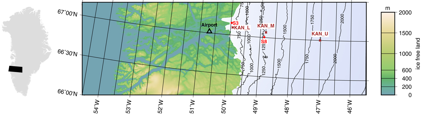
Fig. 1. Weather stations and sampling sites at the K-transect in western Greenland, near the Kangerlussuaq airport (topography data by Morlighem and others (Reference Morlighem, Rignot, Mouginot, Seroussi and Larour2014)). Brown crosses mark the PROMICE weather stations operated by GEUS. Red squares mark additional mass-balance sites where ice samples have been taken close to the PROMICE stations (Wientjes and others, Reference Wientjes2012). Station KAN_U (1840 m a.s.l.) is located near the equilibrium line. Locations S8 and KAN_M (1270 m a.s.l.) are located in the ‘dark region’ with a lower albedo.
Accumulation in the K-transect is low compared with other parts of the GrIS (Burgess and others, Reference Burgess2010). At low elevation near station KAN_L (680 m a.s.l.) snow is redistributed by wind into gullies and crevasses (van den Broeke and others, Reference van den Broeke, Smeets, Ettema and Munneke2008a), causing ice exposure throughout the melting season, while at higher elevations ice is covered by snow in the beginning of the melt season and exposed later on; and, above the equilibrium line, ice is never exposed.
A peculiar area named ‘dark region’ persists below the equilibrium line each melt season. The region is ~30 km wide and starts at ~30 km away from the margin (Wientjes and Oerlemans, Reference Wientjes and Oerlemans2010). Previously the cause of this dark region was believed to be meltwater (Zuo and Oerlemans, Reference Zuo and Oerlemans1996), but now it is attributed to dust (Wientjes and Oerlemans, Reference Wientjes and Oerlemans2010) and carbonaceous particles (Wientjes and others, Reference Wientjes2012). The occurrence of a dark area, the available data as well as the ice exposure make the K-transect an attractive test location for our model.
2. MODEL DESCRIPTION
2.1. Model framework and setup
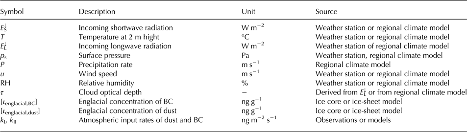
The model simulates daily surface albedo, impurity loadings, snow thickness and SMB for a unit square metre on an ice sheet or glacier and requires the inputs listed in Table 1. In general, our model can be forced by regional climate model output, while in this study we use AWS data in order to optimise the parameters and test the model directly with measurements.
Table 1. Required forcings for the model.
Our model framework consists of seven components shown in Figure 2 and the common parameters are listed in Table 2. The model is developed in Mathematica (version 10, Wolfram Research, Inc., 2014) using self-coded solvers for the differential equations, with a time step of 1 day. The following sections describe each component in advancing order of the flow chart.
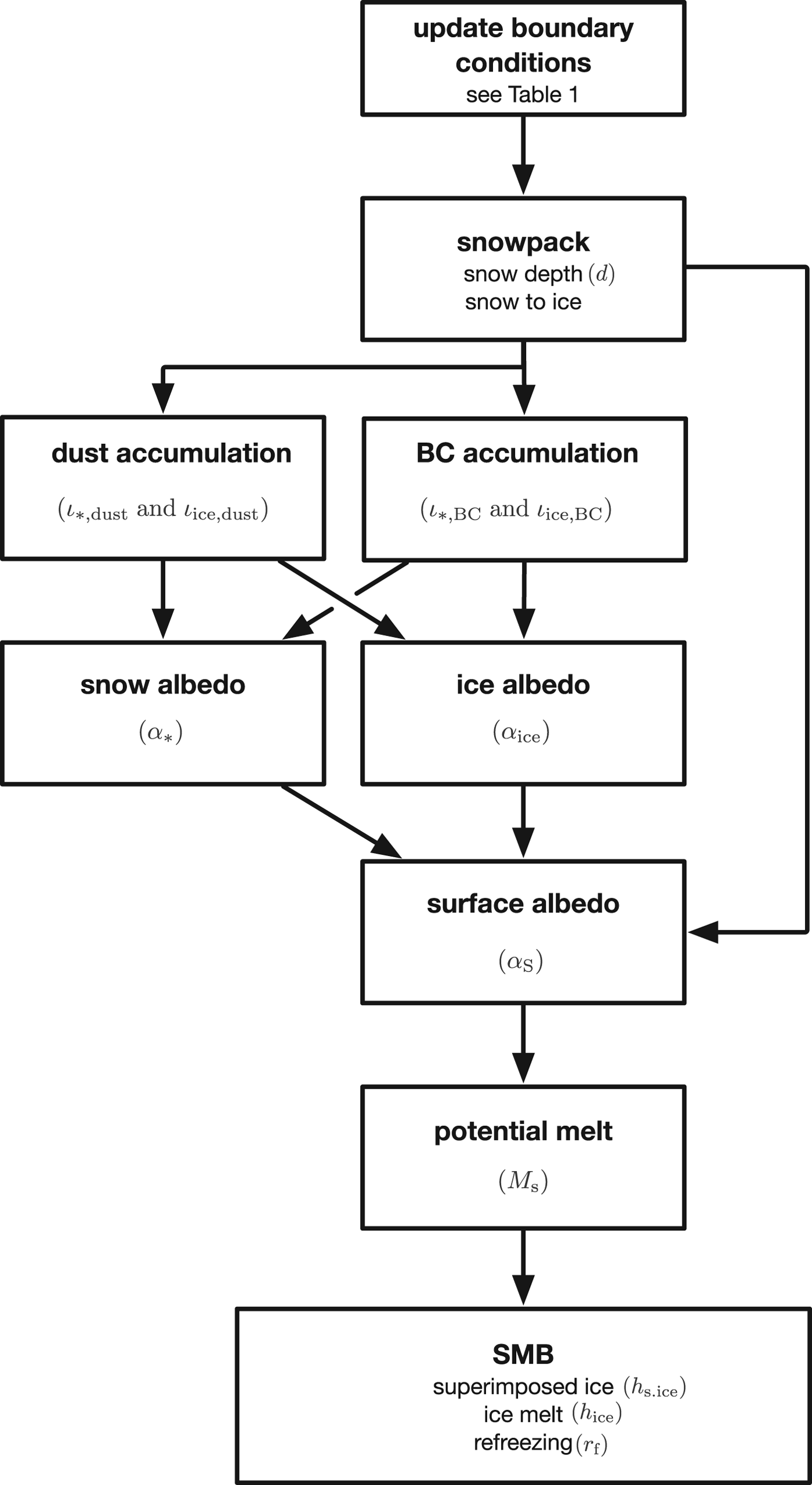
Fig. 2. Flow chart of the surface albedo and surface mass-balance model for a time step of 1 day.
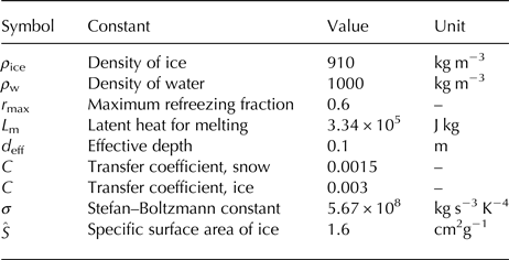
Table 2. Standard physical parameters.
2.2. Snowpack
Snow depth (d) is required for the final SMB, and in order to distinguish between snow and ice surface. It is calculated by a balance between the solid precipitation rate P solid and the melt rate M s (Robinson and others, Reference Robinson, Calov and Ganopolski2010):
 $$ \displaystyle{{\rm d} \over {\rm d}t} d = P_{\rm solid} - M_{\rm s}\comma \quad d \in \lpar 0\comma\; d_{\rm max}\rpar . $$
If the snow depth exceeds d max = 5 m w.e. (Robinson and others, Reference Robinson, Calov and Ganopolski2010; Fitzgerald and others, Reference Fitzgerald, Bamber, Ridley and Rougier2012), the snow depth is reset to 5 m and the surplus amount is added to the ice thickness, which accounts for the snow to ice metamorphism in the accumulation zone. The melt rate is obtained by considering the surface energy balance and is described in Section 2.7. The solid precipitation rate P solid in (1) is based on a temperature-dependent fraction f(T) and the total precipitation rate P (Robinson and others, Reference Robinson, Calov and Ganopolski2010):
 $$ P_{\rm solid} = P \times f\,(T)\comma $$
where the surface temperature-depending fraction f(T) is empirically based on data of Greenland (Calanca and others, Reference Calanca, Gilgen, Ekholm and Ohmura2000; Bales and others, Reference Bales2009) and states that below a minimum temperature (T min = −7°C) all precipitation is snow and above a maximum temperature (T max = +7°C) rain:
 $$\eqalign {& f\lpar T\rpar = \matrix{ 1\comma \hfill & T \lt T_{\rm min}\comma \cr 0\comma \hfill & T \gt T_{\rm max}\comma \cr \cos\left({\displaystyle{{ T-T_{\rm min}} \over {T_{\rm max} - T_{\rm min}}}}\right)\left({\displaystyle {\pi \over 2}}\right)\comma \hfill & T_{\rm min} \lt T \lt T_{\rm max}.} }$$
2.3. Impurity accumulation
Particulate impurities such as BC and mineral dust as well as microbial material have four different sources (Fig. 3):
-
• Atmosphere – distant sources: (k I) by dry or wet deposition,
-
• Atmosphere – local sources: (k II) by regionally transported material from the surrounding tundra,
-
• Flow: (k III) by transport from the accumulation zone to the ablation zone where impurities meltout,
-
• Biological: (k IV) by local biological production of organic material on the ice or snow surface.
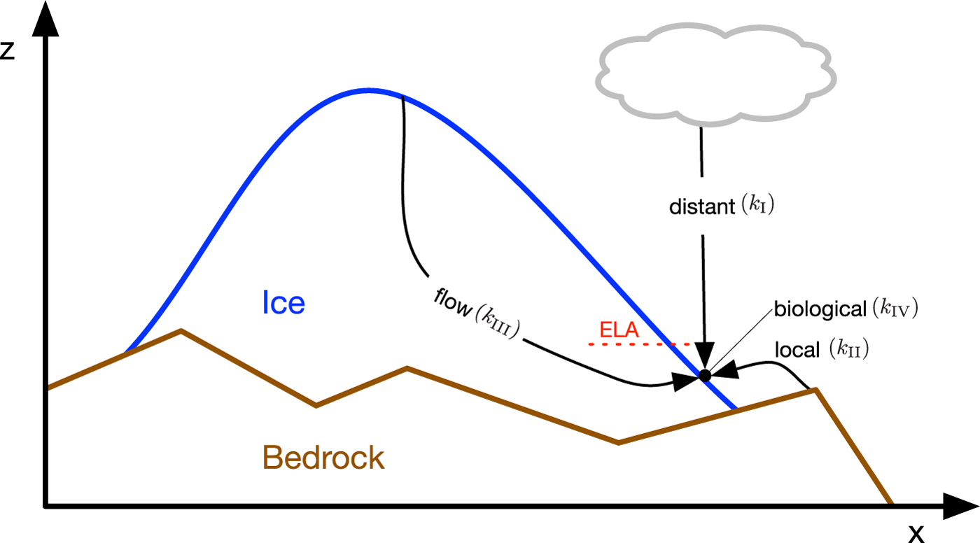
Fig. 3. Cross section through an ice sheet showing the four different sources of impurities in the ablation zone. ELA stands for equilibrium line altitude.
The magnitude of each source depends on the impurity species. The biological source k IV is only relevant for organic matter associated with microbial production. Organic matter was found to contribute only ~5% to the impurity mass on the ablation zone of the GrIS (Bøggild and others, Reference Bøggild, Brandt, Brown and Warren2010; Wientjes and others, Reference Wientjes, van de Wal, Reichart, Sluijs and Oerlemans2011; Takeuchi and others, Reference Takeuchi, Nagatsuka, Uetake and Shimada2014). Due to its relative low concentration and unknown effect on absorption we omit the biological production for now. Nevertheless, we still prepare the impurity accumulation in a way that biological activity can be included in future versions of the model.
The atmospheric sources (k I and k II) contribute to BC and dust accumulation both at higher elevations of the ice sheet and at the margin, while the meltout of englacial impurities, source k III, only contributes in the ablation zone and when ice melts. The following equations are valid for BC (n = BC) and dust (n = dust).
Both atmospheric sources contribute directly to the impurity mass inside the snowpack ι *,n (ng m−2) as well as the local biological production. The vertical distribution inside the snowpack is not considered, which is not necessary since the effect of impurities on snow albedo is not included in the model.
We assume that impurities remain within the snowpack after deposition. Therefore, the impurity concentration inside the snowpack is described by
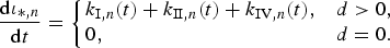 $$\eqalign {\displaystyle{{{\rm d} \iota_{{\ast} \comma n}} \over {{\rm d}t}} & = \left\{ \matrix {k_{{\rm I}\comma n} \lpar t\rpar + k_{{\rm II}\comma n}\lpar t\rpar + k_{{\rm IV}\comma n}\lpar t\rpar \comma \hfill & d \gt 0 \comma \cr 0\comma \hfill & d = 0.}\right. }$$
As ice is exposed (i.e. at snow depth d = 0) englacial impurities and the atmospheric sources and local production all contribute to the impurity mass on the ice surface ι ice, n (ng m−2). The impurity accumulation is counteracted by a reduction term (ν ice(t) ι ice, n ), which is the removal by liquid water and is assumed to be the same for dust and BC. Ideally, ν ice(t) changes with time and includes removal by rain and meltwater, but it is kept constant in this study due the currently limited knowledge about the surface processes. We assume no resuspension of impurities to the atmosphere, because the surface on which they reside is either wet or frozen. Further, we assume that once the snow cover disappears all the impurities in the snowpack are instantly added to the impurity content of the ice surface and no upward impurity flux from ice to snow:
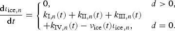 $$\eqalign {\displaystyle{ {\rm d} \iota_{{\rm ice}\comma n} \over {\rm d}t} & = \left\{ \matrix{ 0\comma \hfill & d \gt 0 \comma \cr k_{{\rm I}\comma n}\lpar t\rpar + k_{{\rm II}\comma n}\lpar t\rpar + k_{{\rm III}\comma n}\lpar t\rpar \cr + k_{{\rm IV}\comma n}\lpar t\rpar - \nu_{{\rm ice}}\lpar t\rpar \iota_{{\rm ice}\comma n}\comma \hfill & d = 0.}\right. }$$
The contribution of meltout of englacial impurities k III, n (t), originating from ice flow, depends on the melt rate of ice and the englacial impurity concentration [ι englacial,n ] (the square brackets denote fractions of weight in ppmw). We assume that the impurity content in superimposed ice (h s.ice) is neglectable, since observations indicate a very small impurity concentration in superimposed ice (Chandler and others, Reference Chandler, Alcock, Wadham, Mackie and Telling2015) and impurities only accumulate on the snow surface during melt:
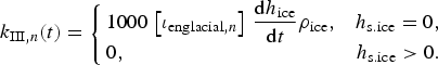 $$\eqalign {k_{{\rm III}\comma n}\lpar t\rpar & = \left\{ \matrix{ 1000 \, \left[ \iota_{{\rm englacial}\comma n}\right] \, \displaystyle {{\rm d} h_{\rm ice} \over {\rm d} t} \rho_{\rm ice}\comma \hfill & h_{{\rm s}.{\rm ice}} = 0 \comma \cr 0\comma \hfill & h_{{\rm s}.{\rm ice}} \gt 0.} \right. }$$
where k III,n (t) is in ng m−2, h ice is the thickness of ice (see 2.8) and ρ ice is the density of ice in kg m−3.
2.4. Ice albedo
The albedo of ice depends on its specific surface area $\hat {S}$
, the effects of impurities (d
α
c), the zenith angle of the sun (dα
θz
) and clouds (dα
clouds). Gardner and Sharp (Reference Gardner and Sharp2010) developed a parameterisation based on experiments with a radiative transfer model of snow and ice coupled to a similar model of the atmosphere:
$\hat {S}$
, the effects of impurities (d
α
c), the zenith angle of the sun (dα
θz
) and clouds (dα
clouds). Gardner and Sharp (Reference Gardner and Sharp2010) developed a parameterisation based on experiments with a radiative transfer model of snow and ice coupled to a similar model of the atmosphere:
 $$\eqalign { \alpha_{\rm ice}= \alpha_{\hat {S}} + {\rm d} \alpha_{\rm c} + {\rm d} \alpha_{\theta_z} + {\rm d} \alpha_{\rm clouds}\comma }$$
where $\alpha _{\hat {S}}$
is the albedo of clean ice with a zenith angle of 0 and no clouds. It is determined by the specific surface area
$\alpha _{\hat {S}}$
is the albedo of clean ice with a zenith angle of 0 and no clouds. It is determined by the specific surface area $\hat {S}$
of ice in cm2 g−1, which depends on the size and distribution of air bubbles and cracks (Gardner and Sharp, Reference Gardner and Sharp2010)
$\hat {S}$
of ice in cm2 g−1, which depends on the size and distribution of air bubbles and cracks (Gardner and Sharp, Reference Gardner and Sharp2010)
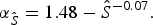 $$\alpha_{\hat {S}} = 1.48 - {\hat {S}}^{- 0.07}. $$
In this study, we use a specific surface area of 1.6 cm2 g−1 for ice with a density of 894 kg m−3 (Dadic and others, Reference Dadic, Mullen, Schneebeli, Brandt and Warren2013). The albedo reduction due to BC is modelled by the equation (Gardner and Sharp, Reference Gardner and Sharp2010)
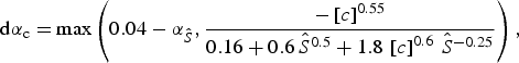 $$\eqalign { {\rm d} \alpha_{\rm c} = & \max \left(0.04 - \alpha_{\hat {S}}\comma \displaystyle {-\left [ c \right ] ^{0.55}\over 0.16 + 0.6\, {\hat {S}}^{0.5} + 1.8\, \left [ c\right ] ^{0.6}\, {\hat {S}}^{-0.25}} \right)\comma }$$
which is designed for concentrations of BC (c in ppmw), and the effect of dust can be included by adding a BC equivalent term. We use a scaling factor of 1/200 to account for the lower absorption of dust (Gardner and Sharp, Reference Gardner and Sharp2010; Dang and others, Reference Dang, Brandt and Warren2015). We define an effective concentration of BC and dust, which accounts for both englacial impurities and impurities located on the ice surface:
 $$ \left [ c\right ] = \left [ \iota_{{\rm eff}\comma BC}\right ] + \left [ \iota_{{\rm eff}\comma {\rm dust}}\right ] \times 1/200\comma $$
where [ι
eff, n
] is the effective aerosol concentration in ppmw, which depends on the englacial concentration as well as the active component of the impurities located at the ice surface. A fraction of impurities can accumulate in cryoconite holes, and be shielded from the low-standing sun of the Arctic (Bøggild and others, Reference Bøggild, Brandt, Brown and Warren2010). This is expressed by the active fraction ${\cal {F}}$
, which is assumed to be the same for BC and dust, in the equation
${\cal {F}}$
, which is assumed to be the same for BC and dust, in the equation
 $$\left [ \iota_{{\rm eff}\comma n}\right ] = \left [ \iota_{{\rm englacial}\comma n}\right ] + \left [ \iota_{{\rm ice}\comma n}\right ] \times {\cal F}\comma $$
where only the active fraction ${\cal {F}}$
contributes to the ice albedo reduction. A value of one means that all impurities are dispersed on the ice surface.
${\cal {F}}$
contributes to the ice albedo reduction. A value of one means that all impurities are dispersed on the ice surface.
The impurity accumulation on ice in (5) is calculated in ng per square metre, while (9) requires fractions of weight (ppmw). We therefore use the following equation to convert between the two quantities:
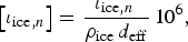 $$\left [ \iota_{{\rm ice}\comma n}\right ] = {\displaystyle{{\iota_{{\rm ice}\comma n}\,} \over {\rho_{\rm ice}\, d_{\rm eff}}}}\, 10^{6}\comma $$
where d eff is the effective depth (in metres). This assumes that impurities on the ice surface have an equivalent effect as the same amount of impurities uniformly distributed in the ice over the effective depth. The upper boundary of the effective depth is linked to the extinction coefficient of ice. At 5 m depth less than 0.1% of the original energy remains, based on an extinction coefficient for clear white ice of 1.6 m−1 (Bøggild and others, Reference Bøggild, Winther, Sand and Elvehøy1995). In contrast, van den Broeke and others (Reference van den Broeke2008b) found that part of the shortwave radiation is absorbed below the surface and causes melting down to 0.45 m. Since the impurities accumulate on the ice surface we assume that the penetration depth is still lower and assume that the shortwave radiation is already absorbed in the first 10 cm. The influence of different effective depths is addressed in Section 3.4.
2.4.1. Clouds
Clouds cause a spectral shift in incident radiation, which increases the albedo with increasing cloud optical thickness τ. The change of albedo caused by clouds is obtained by (Gardner and Sharp, Reference Gardner and Sharp2010)
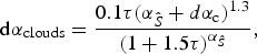 $$ {\rm d} \alpha_{\rm clouds} = {\displaystyle{{0.1 \tau \lpar \alpha_{\hat {S}} + d \alpha_{\rm c}\rpar ^{1.3}} \over {\lpar 1 + 1.5 \tau \rpar ^{\alpha_{{\hat {S}}}} }}\comma}$$
which depends, besides the cloud optical thickness τ, on the specific surface area and the impurity content.
The cloud optical depth is derived from the incoming longwave radiation (E L ↓) (van den Broeke and others, Reference van den Broeke, van As, Reijmer and Van de Wal2004; Munneke and others, Reference Munneke2011):
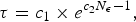 $$\tau = c_1 \times e^{c_2 N_{\epsilon}- 1}\comma $$
where the values of the coefficients c 1 = 2.09 and c 2 = 2.49 are based on data of the K-transect (Munneke and others, Reference Munneke2011, Table 2) and are the mean values of coefficients derived for three stations on similar elevations. The ‘longwave-equivalent cloudiness’ N ε is based on the differences in emissivity of clear and cloudy conditions and is 1 for overcast and 0 for clear conditions. The longwave-equivalent cloudiness is obtained from daily values of incoming longwave radiation and temperature of all stations (N = 6320, period 2009–15 for KAN_M and KAN_L, and 2011–15 for KAN_U).
2.4.2. Zenith angle of the sun
Albedo increases with increasing zenith angle because light is less likely to penetrate deep into ice or snow. Hence, the path length is shorter and the albedo is higher. This is parameterised by (Gardner and Sharp, Reference Gardner and Sharp2010)
 $${\rm d} \alpha_{\theta_z} = 0.53 \alpha_{\hat {S}} \lpar 1 - \lpar \alpha_{\hat {S}} + {\rm d} \alpha_{\rm c}\rpar \rpar \lpar 1 -\cos \theta_z\rpar ^{1.2}\comma $$
where θ z is the zenith angle. Since we use a time step of 1 day we use an insolation-weighted zenith angle for the daily average (e.g. Hartmann, Reference Hartmann2016).
2.5. Snow albedo
We keep snow albedo unaffected by impurities in this study, since the concentrations are low and the effect on surface albedo in the ablation zone is short (see also Fig. S1 in the supplements). The same equations as for ice are used and the effect of clouds and the zenith angle (13 and 15) are still captured:
 $$\alpha_{\ast} = \alpha_{{\hat {S}}\comma \ast} + {\rm d} \alpha_{\theta_z} + {\rm d} \alpha_{\rm clouds}\comma $$
where $\alpha _{{\hat {S}},\,{\ast} }$
is the albedo of snow based on the specific surface area of snow
$\alpha _{{\hat {S}},\,{\ast} }$
is the albedo of snow based on the specific surface area of snow ${\hat {S}},\,\ast $
which changes due to snow metamorphosis. An accurate evolution of
${\hat {S}},\,\ast $
which changes due to snow metamorphosis. An accurate evolution of ${\hat {S}},\,{\ast} $
requires a multi-layer snowpack model and a time step smaller than 1 day. Since we want to keep the snow component as simple as possible, we parametrise the evolution of
${\hat {S}},\,{\ast} $
requires a multi-layer snowpack model and a time step smaller than 1 day. Since we want to keep the snow component as simple as possible, we parametrise the evolution of $\alpha _{{\hat {S}},\,\ast }$
instead. The parameterisation is based on Douville and others (Reference Douville, Royer and Mahfouf1995). During conditions of melt (M
s > 0) the snow albedo decreases exponentially:
$\alpha _{{\hat {S}},\,\ast }$
instead. The parameterisation is based on Douville and others (Reference Douville, Royer and Mahfouf1995). During conditions of melt (M
s > 0) the snow albedo decreases exponentially:
 $$\eqalign {\alpha_{\hat {S}\comma \ast}\lpar t\rpar = \lpar \alpha_{\hat{S}\comma \ast}\lpar t-\Delta t\rpar -\alpha_{\hat{S}\comma \ast\comma {\rm min}}\rpar e^{\tau_{{\rm f}}} + \Delta \alpha_{\hat{S}\comma {\rm fresh}\ast} \comma }$$
while during cold days α * decreases linearly:
 $$\eqalign { \alpha_{\hat{S}\comma \ast}\lpar t\rpar = \alpha_{\hat{S}\comma \ast}\lpar t-\Delta t\rpar - \tau_a + \Delta \alpha_{\hat{S}\comma {\rm fresh}\ast} . }$$
Fresh snow has a higher specific surface area and increases $\alpha _{\hat {S},\,\ast }$
:
$\alpha _{\hat {S},\,\ast }$
:
 $$\eqalign { \Delta \alpha_{\hat{S}\comma {\rm fresh}\ast} & = \left \{\matrix{ 0 \hfill & P_{{\rm solid}}=0 \comma \cr \displaystyle {P_{{\rm solid}} \Delta t\over w_{{\rm crn}}} \lpar \alpha_{\hat{S}\comma \ast\comma {\rm max}}-\alpha_{\hat{S}\comma \ast\comma {\rm min}}\rpar \hfill & P_{{\rm solid}} \gt0.} \right. }$$ $\alpha _{\hat {S},\,\ast }$
is limited between the minimum value
$\alpha _{\hat {S},\,\ast }$
is limited between the minimum value $\alpha _{\hat {S},\,\ast ,\,{\rm min}}$
and the maximum value
$\alpha _{\hat {S},\,\ast ,\,{\rm min}}$
and the maximum value $\alpha _{\hat {S},\,\ast ,\,{\rm max}}$
. The decay parameters τ
f and τ
a influence the albedo reduction since the last snowfall. The parameter w
crn (in m w.e.) determines the increase during snowfall.
$\alpha _{\hat {S},\,\ast ,\,{\rm max}}$
. The decay parameters τ
f and τ
a influence the albedo reduction since the last snowfall. The parameter w
crn (in m w.e.) determines the increase during snowfall.
2.6. Surface albedo
The albedo at a geographical point on a glacier or ice sheet is determined by the surface type, clouds, the solar zenith angle and impurities. If the snow depth is below a critical mark d crit the surface albedo is still influenced by the darker underlaying ice (Fig. 4). Above the critical snow depth d crit the surface albedo is equivalent to the albedo of snow α * (based on (van den Berg and others, Reference van den Berg, van de Wal and Oerlemans2008; Robinson and others, Reference Robinson, Calov and Ganopolski2010)):
 $$\eqalign { \alpha_{{\rm s}} & = \left \{ \matrix{ \alpha_{{\rm ice}}\comma \hfill & d = 0\comma \cr \alpha_{{\rm ice}} + \displaystyle {{d}\over {d}_{{\rm crit}}}\lpar \alpha_{\ast}-\alpha_{{\rm ice}}\rpar \comma \hfill & 0 \lt d< d_{{\rm crit}}\comma \cr \alpha_{\ast}\comma \hfill & d \ge d_{{\rm crit}}. } \right. }$$
This equation allows the snow albedo to be lower than the ice albedo, which could be the case, although rare, when debris-rich wet snow covers clean ice.

Fig. 4. The relationship between ice albedo, snow albedo and impurities to surface albedo (α s). The surface albedo is still influenced by the underlaying ice surface if the snow depth (d) is lower than the critical snow depth (d crit).
2.7. Potential melt
We use an energy-balance model to derive the potential melt rate. Subsurface and heat flux from rain are both insignificant (van As and others, Reference van As2012) in the K-transect, which reduces the surface energy balance to
 $$\eqalign {& E_{{\rm M}}=E_{{\rm S}}^\downarrow \lpar 1- \alpha_{{\rm s}} \rpar + E_{{\rm L}}^\downarrow + E_{{\rm L}}^\uparrow + E_{{\rm H}} + E_{{\rm E}}\comma }$$
where fluxes are positive when they add energy to the surface. The incoming shortwave and longwave radiation E S ↓ and E L ↓ are external inputs. Outgoing longwave radiation E ↑ L is calculated by the Stefan–Boltzmann law with the surface temperature T s. The surface temperature is obtained by balancing the right-hand side. Energy for melt E M is available when the right-hand side can not be balanced, i.e. the surface temperature T s is at the melting point. The turbulent heat fluxes of latent heat E H and sensible heat E E are calculated with different transfer coefficients C for snow and ice (see Table 2) (Cuffey and Paterson, Reference Cuffey and Paterson2010):
 $$ E_{{\rm H}}=0.0129 \, C\, p_{{\rm s}}\, \lpar T-T_{{\rm s}}\rpar \comma$$
 $$E_{{\rm E}} = 22.2 \, C\, u\, \lpar p_{{\rm w}} - p_{{\rm w\comma s}}\rpar \comma$$
where u is the wind speed, p s is the surface pressure and p w is the vapour pressure. The surface vapour pressure p w, s is derived by assuming saturation, p w, s = pw, sat, with (WMO, 2014)
 $$\eqalign { p_{{\rm w\comma sat}} = 611.2\, e^{17.62\, T_{{\rm s}} / \lpar 243.12 + T_{{\rm s}}\rpar } \comma }$$
where p w, sat is in Pa.
The potential melt rate M s is derived from the available energy for melt E M:
 $$M_{\rm s} = \displaystyle{{E_{{\rm M}} \over \rho_{\rm w}\, L_{\rm m}}\comma }$$
where ρ w is the density of water, L m is the latent heat of melting.
2.8. Surface mass balance
The change of ice thickness h ice in m w.e. together with the snow depth forms the SMB component of the model. The equation accounting for refreezing reads (Robinson and others, Reference Robinson, Calov and Ganopolski2010)
 $$\eqalign { \displaystyle{{\rm d} \over {\rm d}t} h_{{\rm ice}} = \left \{\matrix{ M_{{\rm s}} r_{{\rm f}}\comma \hfill & d \gt 0 \comma \cr {\rm min}\, \lpar P_{{\rm solid}}-M_{{\rm s}}\comma 0\rpar \comma \hfill & d=0 \comma } \right. }$$
where r f is the refreezing fraction within the snowpack as a function of the snow depth and the surface temperature T (Robinson and others, Reference Robinson, Calov and Ganopolski2010):
 $$\eqalign { r_{{\rm f}} & = \left \{ \matrix{ 0\comma \hfill & d = 0 \comma \cr r_{\rm max} f\lpar T\rpar \comma \hfill & 0 \lt d \le 1 \comma \cr r_{\rm max}+\left [ \lpar 1-r_{\rm max}\rpar \lpar d-1\rpar \right ] \comma \hfill & 1 \lt d \le 2 \comma \cr 1 \comma \hfill & d \gt 2 . } \right. }$$
When the snow depth is below 1 m the refreezing fraction is determined by the maximum fraction of refreezing r max and the fraction of snow (3). Above 1 m, but below 2 m, the refreezing fraction increases linearly and reaches its maximum at 2 m. The thickness of superimposed ice h s.ice is derived form the first part of (25).
2.9. Calibration and evaluation
We chose the free parameters based on data availability: the snow albedo parameters w
crn, $\alpha _{{\hat {S}},\,\ast ,\,{\rm min}}$
,
$\alpha _{{\hat {S}},\,\ast ,\,{\rm min}}$
, $\alpha _{\hat {S},\,\ast ,\,{\rm max}}$
, τ
f, τ
a, critical snow depth d
crit, the active fraction of BC and dust on ice
$\alpha _{\hat {S},\,\ast ,\,{\rm max}}$
, τ
f, τ
a, critical snow depth d
crit, the active fraction of BC and dust on ice $\cal {F}$
and the reduction fraction on ice ν
ice. The ranges of parameters are shown in Figures 5, 6.
$\cal {F}$
and the reduction fraction on ice ν
ice. The ranges of parameters are shown in Figures 5, 6.
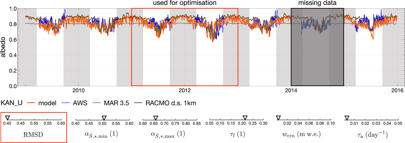
Fig. 5. Albedo model results for station KAN_U from 2009 until the end of 2015 with missing data in 2014. Optimisation of snow parameters is performed on data of 01.01.2011 to 31.12.2012. The remaining period is used to test the albedo model at a location where ice is never exposed. Only data outside the grey areas are used during the optimisation, when radiation data are usually available. Model results are compared with AWS data (blue) and model results of MAR and downscaled results of RACMO. MAR and RACMO albedo are smoothed with a running average over 7 days to improve readability of the graph. The lower sections show the resulting parameters and the ranges used during the optimisation.
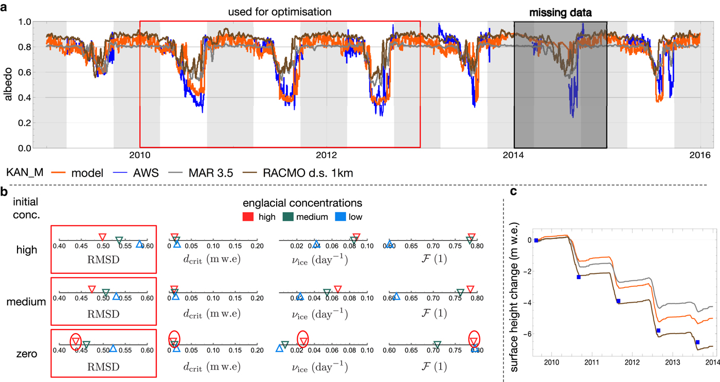
Fig. 6. Model results of station KAN_M from 2009 until the end of 2015 with missing data in 2014. Panel (a) shows the resulting albedo compared with AWS data and simulations of MAR and RACMO. Panel (b) shows the results of the optimisation for nine scenarios of initial impurity loading and englacial concentration. Only data outside the grey areas are used during the optimisation, when AWS data are usually available. The lowest RMSD is obtained with the zero initial and high englacial concentration setting, and is marked by a red circle. The model run (orange) in (a and b) uses this parameter settings and the optimised snow parameters. Panel (c) shows surface height change compared with SMB measurements (blue squares).
Optimisation of the parameters in the equations for $\alpha _{\hat {S},\,\ast }$
is necessary since we apply them to
$\alpha _{\hat {S},\,\ast }$
is necessary since we apply them to $\alpha _{\hat {S},\,\ast }$
rather than the final snow albedo. Therefore, literature values of w
crn,
$\alpha _{\hat {S},\,\ast }$
rather than the final snow albedo. Therefore, literature values of w
crn, $\alpha _{\hat {S},\,\ast ,\,{\rm min}}$
,
$\alpha _{\hat {S},\,\ast ,\,{\rm min}}$
, $\alpha _{\hat {S},\,\ast ,\,{\rm max}}$
, τ
f, τ
a cannot be used.
$\alpha _{\hat {S},\,\ast ,\,{\rm max}}$
, τ
f, τ
a cannot be used.
The critical snow depth determines the rate of change from the summer to the winter surface albedo as well as the change from wet snow to bare ice and is found via the optimisation.
The active fraction $\cal {F}$
bundles all surface processes together and is a free parameter, which accounts for impurity dynamics on the ice surface and cryoconite hole formation. During optimisation
$\cal {F}$
bundles all surface processes together and is a free parameter, which accounts for impurity dynamics on the ice surface and cryoconite hole formation. During optimisation $\cal {F}$
is allowed to vary over the range of 0.6–0.8, which means to 60–80% of the impurities are actively darkening the ice surface. This range of
$\cal {F}$
is allowed to vary over the range of 0.6–0.8, which means to 60–80% of the impurities are actively darkening the ice surface. This range of $\cal {F}$
values is based on unmanned aircraft observations at the K-Transect (Ryan and others, Reference Ryan, Hubbard, Stibal and Box2016) where ~60–80% of the surface was distributed impurities east of station KAN_M. Although this is not directly linked to our meaning of the active fraction, it still is related and reduces the range of expected values for the active fraction.
$\cal {F}$
values is based on unmanned aircraft observations at the K-Transect (Ryan and others, Reference Ryan, Hubbard, Stibal and Box2016) where ~60–80% of the surface was distributed impurities east of station KAN_M. Although this is not directly linked to our meaning of the active fraction, it still is related and reduces the range of expected values for the active fraction.
The runoff fraction on ice is also a free parameter, since it is currently not observed and its range is estimated from observed impurity masses on the GrIS ablation zone (Section 4.2).
The optimisation is done by minimising the RMS deviation (RMSD) between the modelled and observed albedo during the period of 20 March until 20 September when AWS albedo data are available. Optimisation is performed with the Mathematica function ‘NMinimize’, which automatically chooses an appropriate method such as Nelder–Mead, differential-evolution, simulated annealing and random search (Wolfram Research, Inc., 2014), and the process is stopped after a maximum of 1000 iterations.
The optimisation of the parameters is performed in two stages. First, the snow albedo parameters are optimised on data of KAN_U where ice is never exposed. In the second stage, the ice parameters are optimised on data of KAN_M, already using the optimised snow parameters. In the first stage, the parameters w
crn, $\alpha _{\hat {S},\,\ast ,\,{\rm min}}$
,
$\alpha _{\hat {S},\,\ast ,\,{\rm min}}$
, $\alpha _{\hat {S},\,\ast ,\,{\rm max}}$
, τ
f and τ
a are optimised, and in the second stage at KAN_M the critical snow depth dcrit and the active fraction of BC and dust on ice
$\alpha _{\hat {S},\,\ast ,\,{\rm max}}$
, τ
f and τ
a are optimised, and in the second stage at KAN_M the critical snow depth dcrit and the active fraction of BC and dust on ice $\cal {F}$
, the reduction fraction on ice ν
ice.
$\cal {F}$
, the reduction fraction on ice ν
ice.
During optimisation we use the data of 2011/12 at KAN_U and 2010–12 at KAN_M, which leaves the rest of the data, and all the data of station KAN_L, for model evaluation. The simulated albedo is compared with AWS data and simulations of the regional climate models MAR and RACMO. MAR (v3.5.2) uses NCEP-NCARv1 reanalysis forcings (Fettweis and others, Reference Fettweis2017) and gives results on a 20 km grid, which we bilinearly interpolated to the AWS locations. RACMO uses ERA-40 and ERA-Interim forcings, and the native 11 km grid has been downscaled to 1 km (v2.3, Noël and others, Reference Noël2016) by using the values of the nearest grid point. In addition, SMB is compared with observations (Machguth and others, Reference Machguth2016) and simulations of MAR and RACMO.
2.10. Boundary conditions and initial conditions
The model requires initial values of snow depth and impurity surface concentration, in addition to the boundary conditions mentioned in Table 1. The initial snow depth is derived from sonic ranger data and are: at KAN_L 0.2 m w.e. on 01.01.2009, at KAN_M 0.5 m w.e. on 01.01.2009 and 0.25 m w.e. on 01.01.2010. For KAN_U, close to the equilibrium line, the initial snow depth is arbitrary set to 2 m, which does not effect the result, since ice is never exposed there.
Since direct observations of surface concentrations are lacking, we use three scenarios of initial surface concentrations during optimisation; one each for high, medium and no initial impurity loadings, respectively. In all scenarios, the initial snow impurity concentrations are zero, since model snow albedo is unaffected by impurities and impurity loadings on snow are comparably low.
The ‘high’ initial scenario corresponds to 200 g m−2 dust and 1 g m−2 BC, and the ‘medium’ scenario corresponds to 50 g m−2 dust and 0.1 g m−2 BC.
All the atmospheric boundary conditions in Table 1 are provided by the AWS, besides the precipitation which comes from MAR. The atmospheric input rate from distant sources (k I) of BC is 0.001 g m−2 a−1 obtained from ice cores (Lee and others, Reference Lee2013). For dust the atmospheric input rate is 0.01 g m−2 a−1, based on model simulation (Mahowald and others, Reference Mahowald, Albani, Engelstaedter, Winckler and Goman2011) and ice core analysis (Albani and others, Reference Albani2015). The local atmospheric input (k II) for both dust and BC is set to zero, since we do not distinguish between those two sources at the moment.
Similar to the three scenarios for initial conditions, the optimisation at KAN_M is performed with three scenarios of englacial concentrations based on the available data of BC (ice samples at S1 and S8, Wientjes and others, Reference Wientjes2012) and dust (Ruth, Reference Ruth2007). The scenario with high englacial concentrations uses 4 ng g−1 BC and 3000 ng g−1 dust, the medium concentrations scenario uses 2 ng g−1 BC and 1000 ng g−1 dust and the low concentration scenario 0.5 ng g−1 BC and 10 ng g−1 dust. These three englacial concentrations scenarios are applied to each initial condition scenario.
At KAN_L the BC concentration is 1 ng g−1, based on the nearby S1 core (Wientjes and others, Reference Wientjes2012). The dust concentration is 200 ng g−1 at KAN_L, based on NGRIP (Ruth, Reference Ruth2007) and the location outside the dark area.
3. MODELLING RESULTS
3.1. Calibration
Figure 5 presents the station KAN_U with the results of the optimised snow albedo parameters and the corresponding simulated albedo (for SMB see Fig. S2 in the supplements). The obtained values are 0.506 for $\alpha _{\hat {S},\,\ast ,\,{\rm min}}$
, 0.660 for
$\alpha _{\hat {S},\,\ast ,\,{\rm min}}$
, 0.660 for $\alpha _{\hat {S},\,\ast ,\,{\rm max}}$
, 0.215 for τ
f, 0.0034 m w.e. for w
crn and a reduction of
$\alpha _{\hat {S},\,\ast ,\,{\rm max}}$
, 0.215 for τ
f, 0.0034 m w.e. for w
crn and a reduction of $\alpha _{\hat {S},\,\ast }$
during dry conditions (τ
a) of 0.003 day−1.
$\alpha _{\hat {S},\,\ast }$
during dry conditions (τ
a) of 0.003 day−1.
Figure 6 shows the optimisation result of the ice albedo parameters. The scenario with no initial impurities and high englacial concentrations gives the lowest deviation from albedo measurements. Therefore, this scenario delivers the best estimates of the parameters, which are 0.009 m w.e. for the critical snow depth dcrit, 0.028 day−1 for the reduction fraction on ice ν
ice and 0.792 for the active fraction $\cal {F}$
.
$\cal {F}$
.
3.2. Evaluation
The model is evaluated at all stations. At KAN_U (Fig. 5) modelled albedo is in good agreement with data, also outside the period, which was used for optimisation. The observed SMB during the period 2011–2014 is slightly negative, while all the models, MAR and RACMO and ours similarly produced a slightly positive SMB (Fig. S2 in the supplements).
At station KAN_M in Figure 6 (panel c) the simulated SMB is lower than the observed one and is between MAR and RACOMO. The simulated albedo follows the AWS data during summer when ice is exposed, while MAR and RACMO display a 0.2 too high ice albedo of ~ 0.6.
At lower elevations at KAN_L (Fig. 7) the albedo of ice is ~ 0.5 each summer. All models succeeded in a similar way to reproduce the ice albedo in summer, while all models failed to catch the variations in spring, which are lager than at KAN_M and likely caused by drifting snow. The resulting SMB at KAN_L of our model is between the other models, but lower than the observations (Fig. S3).
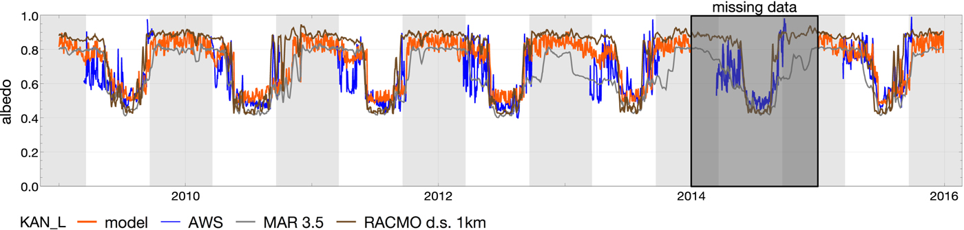
Fig. 7. Simulated and observed albedo at KAN_L with the model parameters from the optimisation at KAN_M and KAN_U and the englacial concentration of BC of 1 and 200 ng g−1 dust.
3.3. Station KAN_M in 2010
Figure 8 displays the simulations of the KAN_M station in the year 2010 in more detail, where the initial snow depth is set to 0.25 m w.e. (panel e) based on sonic ranger data and simulated snow depth is converted to metres with a snow density of 650 kg m−3. While in Figure 6 the snow depth on 01.01.2010 is a result of the snow depth evolution in 2009 (0.34 m w.e.). All initial impurity concentrations are zero, according to the best scenario in Figure 6.

Fig. 8. Detailed results of station KAN_M in 2010. (a) Near-surface temperature from AWS, (b) daily precipitation from regional climate model MAR (c and d) show the evolution of dust (red) and BC (black) inside the snowpack and on the ice surface. Panel (e) shows snow depth evolution of the models and derived from sonic ranger data. (f) Surface type; s.i. ice stands for superimposed ice. (g) Surface albedo evolution of data and simulations. The AWS data in thick blue, MAR and RACMO simulations are smoothed (over 7 days). Panel (h) shows the albedo of snow and ice due to changes in the specific surface area. Panels (i–k) show components of the albedo for both snow and ice.
The amount of dust and BC inside the snowpack (panel (c)) builds up until all the snow has melted in late June (panel (e)). All the impurities from the snowpack are deposited on the ice surface, causing a jump of BC concentration in (d), while the input of dust from snow is comparably small and is not visible in (d).
When ice is exposed there is an influx of impurities from meltout and the constant atmospheric deposition. In late September, the amount of dust decreases because the amount of impurity loss exceeds gain by meltout and atmospheric deposition.
Panels (i–k) show the evolution of the albedo components of ice and snow. Panel (i) shows the increasing darkening effect of impurities on the albedo of ice caused by accumulating dust and BC. The effect of clouds on ice is smaller than that on snow due to the lower specific surface area of ice. One significant summer snowfall event is visible in late August, which the model captures, although with a too high albedo.
The simulated maximum amount of BC on the ice surface is 0.006 g m−2 and of dust is 1.7 g m−2. Hence, the mass of dust on the ice surface is 270 times larger than BC. The maximum amount in the snowpack is 0.31 mg m−2 BC and 3.12 mg m−2 dust.
3.4. Sensitivity
Figure 9 shows surface height change relative to the optimised setting. The boundary conditions are from KAN_M at 2010 repeated over 5 years. The sensitivity experiments are compared with the settings of KAN_M at 2010, described above. Corresponding plots of albedo and impurity loading can be found in Figure S5 in the supplements.

Fig. 9. Simulations of surface height change relative to the optimised settings at KAN_M 2010 (orange) in (a). Panel (b) shows a zoom in on (a).
Atmospheric input has only a small effect on the final SMB, as can be seen in the experiment when atmospheric input is turned off (brown line). On the other hand, if meltout of impurities is prohibited the loss is about 4 m w.e. lower than the reference. Similarly changes in englacial concentrations have a significant effect on the SMB.
The upper limit of the effective depth d
eff of 5 m causes less mass loss after 5 years, since it influences the effect of impurities on the albedo of ice. Next, the specific surface area of ice has big effects on SMB. A 0.6 cm2 g−1 lower specific surface area of ice causes 1.8 m w.e. more ice loss. A much higher specific surface area $ \hat {S} $
of 10 cm2 g−1, i.e. ice with more air bubbles, causes a brighter surface and a smaller effect of impurities. Therefore, the specific surface of 10 cm2 g−1 causes more than 8 m w.e. less ice loss, compared with the reference.
$ \hat {S} $
of 10 cm2 g−1, i.e. ice with more air bubbles, causes a brighter surface and a smaller effect of impurities. Therefore, the specific surface of 10 cm2 g−1 causes more than 8 m w.e. less ice loss, compared with the reference.
A higher reduction fraction ν ice of 0.05 causes impurities to runoff faster and therefore causes about 1 m w.e. less ice loss after 5 years due to a higher albedo. Similarly, a smaller ν ice of 0.001, or 0.1% impurity mass loss per day, causes impurities to build up and an albedo decrease of 0.2 (Fig. S5).
In the next test, the surface temperature is increased by 2 and 5 K, with and without meltout of impurities. The effect of temperature on mass loss is negative and more negative when meltout is considered. This is a result of longer ice exposure and additional meltout caused by the higher temperatures (Fig. S5). At 5 K higher temperatures the difference between prohibited and activate meltout is 10 m w.e.
Finally, a different conversion factor between dust and BC is investigated. The lower factor of 1/100 causes a higher mass loss of ~1.8 m w.e., while a factor of 1/300 causes 0.8 m w.e. less mass loss.
4. DISCUSSION
4.1. Assumptions and uncertainties
We now briefly discuss the assumptions and uncertainties of each model component of the order of the flow chart (Fig. 2).
The snowpack component is a simple, one-dimensional model, which does not account for density changes or the evolution of the specific surface area due to snow metamorphosis. The snow-depth determines the time of ice exposure and therefore the timing when impurities can accumulate. The lower initial snow depth in Figure 8 caused a lower albedo, which matched observations better, compared with Figure 6, where a too high snow depth was carried over from 2009.
The next component to discuss is the impurity accumulation inside the snowpack and on the ice surface. The impurity accumulation inside the snowpack in our model depends solely on the atmospheric inputs and biological production. Since the atmospheric fallout rates of both BC and dust are low, the impact on the albedo of snow is also low (see also Fig. S1). The constant influx of dust and BC is a simplification – in nature the influx of impurities is very erratic – as can be seen in ice core records (McConnell and others, Reference McConnell2007; Ruth, Reference Ruth2007). Therefore, the impurity concentration inside the snowpack also follows this highly variable behaviour in nature. In order to account for this in the model, a more sophisticated treatment of snow albedo would be required. This could be achieved with a multilayer snowpack model together with impurity deposition determined by an atmospheric model.
The scenarios of the initial impurity concentration and englacial concentrations indicate that the initial impurity loading was likely low in combination with high englacial concentrations. Short ice cores and surface concentration measurements are required to better constrain the model and make these scenarios unnecessary. In addition, time-lapse cameras on the weather stations and frequent measurements of surface concentrations could be used to gain insight and derive a more physical handling of impurity loss and lateral movement.
Changes in the reduction fraction have a big impact on the magnitude of accumulated impurities (Figs 9, S5). Three years for optimisation is considered too short to be confident in the reduction fraction ν ice. The reduction fraction varied over the entire range in Figure 6b. In addition the reduction term in this study is a simplification, because removal of impurities most likely varies with particle size and depends on meltwater production and rainfall.
The snow albedo in general is in good agreement with observations, despite its simple parameterisation. The daily variation in snow albedo was higher than in observations, which is most likely caused by the effect of clouds (Fig. 8k) and depends on the cloud optical depth derived from longwave radiation data and $\alpha _{\hat {S},\,\ast }$
, which was parametrised. A model of specific surface area evolution of snow could be used to derive
$\alpha _{\hat {S},\,\ast }$
, which was parametrised. A model of specific surface area evolution of snow could be used to derive $\alpha _{\hat {S},\,\ast }$
, which would also enable consideration of impurities on snow. Currently the impurity effect on snow is zero, which causes an overestimation of the effect of clouds; see (13). However, despite the simplicity of the snow albedo component it captures the termination of the snow cover and hence provides a realistic initiation of glacier ice melt.
$\alpha _{\hat {S},\,\ast }$
, which would also enable consideration of impurities on snow. Currently the impurity effect on snow is zero, which causes an overestimation of the effect of clouds; see (13). However, despite the simplicity of the snow albedo component it captures the termination of the snow cover and hence provides a realistic initiation of glacier ice melt.
A high uncertainty affecting the ice albedo is the active fraction $\cal {F}$
, which is linked to cryoconite hole development. An additional uncertainty is caused by the conversion of surface concentrations to ng g−1 using the effective depth deff. The parameterisation of ice albedo (9) assumes an external mixture of carbon particles (located outside of ice grains, Gardner and Sharp (Reference Gardner and Sharp2010)). We assumed that particles located on the ice surface have a similar effect on albedo as this external mixture. This might be an oversimplification, which most likely will not hold at very high surface concentrations, when most of the radiation is absorbed by particles on the surface. For example, a layer of dust thicker than 1.33 mm insulates the ice surface (Adhikary and others, Reference Adhikary, Nakawo, Seko and Shakya2000) and therefore reduces melt. A dust layer this thick corresponds to a surface concentration of the order of kg m−2, while at stations KAN_M and KAN_L the total simulated impurity loading was only of the order of a few g m−2. Nevertheless, a study of impurities located on the ice surface is required in order to improve the active fraction and the conversion. Ideally, this would make the conversion obsolete, so that the ice albedo could directly be related to surface concentrations.
$\cal {F}$
, which is linked to cryoconite hole development. An additional uncertainty is caused by the conversion of surface concentrations to ng g−1 using the effective depth deff. The parameterisation of ice albedo (9) assumes an external mixture of carbon particles (located outside of ice grains, Gardner and Sharp (Reference Gardner and Sharp2010)). We assumed that particles located on the ice surface have a similar effect on albedo as this external mixture. This might be an oversimplification, which most likely will not hold at very high surface concentrations, when most of the radiation is absorbed by particles on the surface. For example, a layer of dust thicker than 1.33 mm insulates the ice surface (Adhikary and others, Reference Adhikary, Nakawo, Seko and Shakya2000) and therefore reduces melt. A dust layer this thick corresponds to a surface concentration of the order of kg m−2, while at stations KAN_M and KAN_L the total simulated impurity loading was only of the order of a few g m−2. Nevertheless, a study of impurities located on the ice surface is required in order to improve the active fraction and the conversion. Ideally, this would make the conversion obsolete, so that the ice albedo could directly be related to surface concentrations.
The active fraction varied over almost the entire range (Fig. 6b) between 0.6 and 0.8 and is uncertain. The uncertain initial surface concentrations and englacial concentrations cause the active fraction to vary. The high active fraction of 0.792 is at the upper limit of the range, and is an indication that the initial concentration or englacial concentration are too low. Therefore, direct measurements of the englacial and surface concentration and observations of dust and BC deposition can further constrain the active fraction. The active fraction itself could possibly be obtained by time-lapse cameras and further studies on the dynamics of cryoconite holes and the dynamics of dispersed impurities. For now, the active fraction bundles all surface processes together, but it could be a model component on its own in the future.
The zenith angle of the sun has a high impact on the albedo of ice and snow. The slope of the GrIS is small and therefore has little effect on the effective zenith angle, while this is not the case for steep valley glaciers. In this study, we use a daily time step and calculated the zenith angle by an insolation-weighted daily mean. A smaller time step could be used to improve the effect of the zenith angle and include diurnal variations. Other uncertainties influence the effect of the zenith angle, because the associated albedo variation depends on the specific surface area and the effect of impurities (15).
The free parameter of the surface albedo component (20) is the critical snow depth, which only varied over a narrow range in all nine scenarios and therefore has a low uncertainty.
The simulated surface concentrations are within the range of observations of 0.36–1400 g m−2, although they most likely are too low. Besides initial concentrations, atmospheric inputs, englacial concentrations and the surface concentrations also depends on melt rates, which makes it dependent on all the other uncertainties. Therefore, the confidence in the simulated surface concentration is low. Nevertheless, simulating the exact surfaces concentration was not the goal. Routinely observations of surface concentrations near the AWS could be used to better constrain the model and improve the overall performance.
Biogenic matter was not included during optimisation of the free parameters. This adds uncertainty to the optimised free parameters of the active fraction and reduction fraction, as dark biogenic material and in situ production was neglected.
Overall, the performance of the model is satisfying, because the albedo at all three stations approximated observations well and the quality of SMB simulations was similar to MAR and RACMO. This shows the potential of the model framework and should motivate further studies on ice surface processes and impurity concentrations and dynamics.
4.2. Runoff of impurities and residence time
As discussed above, the confidence in the value of the reduction fraction is rather low. Therefore, we investigated equilibrium surface concentrations of dust, i.e. when the amount of accumulation of dust is balanced with the amount of dust loss. The surface concentration still varies during ice exposure, but otherwise is constant each year after equilibrium is reached. In nature, the system is very dynamic as a result of weather and dust influx, both from atmosphere and from meltout. Nevertheless, the equilibrium surface concentrations compared with the observed surface concentrations gives further insight in the magnitude of the reduction fraction.
In the extreme case of no englacial dust, it would take a reduction fraction as low as 0.0001 to reach just 1 g m−2 of dust (see Fig. S6a in the supplements). On the other extreme with an englacial concentration of 5000 ng g−1, the same reduction fraction of 0.0001 would cause a surface concentration of above 1 kg m−2, which has been observed in North-east Greenland (Bøggild and others, Reference Bøggild, Brandt, Brown and Warren2010). Taking the same high englacial concentration and a reduction fraction of 0.05 results in an equilibrium dust concentration of 1.8 g m−2.
By assuming 60 days of ice exposure and no additional influx, it would take only about 3 years to reduce from 100 g m−2 to below 1 g m−2 with the optimised reduction fraction of 0.028 day−1. On the other hand, it would take almost 1000 years to reduce from 100 to below 1 g m−2 with a reduction fraction of 0.0001 (Fig. S6b).
Our optimised reduction fraction is most likely at the high end, as it results in an equilibrium surface concentration of dust below 100 g m−2, even at extreme englacial concentrations and high rates of atmospheric deposition (Fig. S6a). Further studies of the dynamics of dispersed impurities are required to derive a better representation of impurity runoff and redistribution.
4.3. Meltout of impurities
What is the dominant source of dust and BC on the ice surface?
One metre of ice melt releases englacial impurities, which have been deposited over multiple years or decades in the accumulation zone several thousand years ago.
Dust concentrations in ice formed during the last glacial are 10–100 times higher than in ice formed during the Holocene (Steffensen, Reference Steffensen1997). For example, melt of 1 metre of ice with a dust concentration of 1000 ng g−1 releases 0.91 g m−2 of dust. At the current rate of atmospheric deposition from large-scale transport it would take about 100 years to deposit the same amount of dust from the atmosphere directly (Fig. S7 in the supplements). Therefore, meltout is the main source of dust on the ice surface, which is also supported by a study of the isotopic composition (Nagatsuka and others, Reference Nagatsuka2016).
Atmospheric deposition of local dust could play a significant role close to the margin if the transport by wind from the surrounding tundra is effective. The local dust source is likely restricted to the outermost ablation zone because of the prevailing katabatic winds. Therefore, there might be a ‘threshold elevation’ up to which local dust from the tundra contributes significantly. Above this threshold, large-scale transport from distant sources dominates.
For BC the pattern is less clear. Local sources can be neglected because Greenland has a population of only approximately 50 000 along the entire western flank of the ice sheet and no forest exists. Ice formed between 1851 and 1951 has a mean concentration of BC of 4 ng g−1, while the preindustrial concentration is 1.7 ng g−1 (McConnell and others, Reference McConnell2007). Atmospheric deposition is the dominant source of BC, up to annual melt rates of 1 m and a BC concentrations of 1.0 ng g−1 (Fig. S6b). At higher melt rates melt-out of BC dominates, but the atmospheric deposition still contributes significantly to the amount of BC on the ice surface.
The sensitivity analysis in Figure 9 shows that without atmospheric deposition the mass loss was <0.2 m w.e. lower compared with the reference. When prohibiting melt-out the mass loss was almost 4 m w.e. lower after the same period.
5. CONCLUSIONS
We developed a surface mass-balance model with a dynamic ice albedo component. In our model, ice albedo is affected by the accumulation of dust and BC, clouds and the zenith angle of the sun. The model is forced with data from weather stations and compared with observations of albedo and SMB. A sensitivity evaluation showed that the model is most sensitive to changes in englacial concentrations, which determines the amount of impurities released by melt.
Dust is the main contributor to impurity by mass, of which meltout is the main source. Meltout of BC is the dominant source at annual melt rates above 1 m. Nevertheless, current atmospheric deposition of BC contributes considerably to the total amount of BC on the ice surface. Therefore, mitigation of BC emissions outside of Greenland has an immediate effect on the albedo of the ice surface. The scarce population and lack of forest in Greenland eliminate the local BC source.
Glacier ice albedo and its linkage to impurity dynamics on the surface has never been quantified in this detail before and the lack of necessary input data is obviously present. We have to the best ability applied in situ measurements and have carefully evaluated free parameters based on thorough field experience. The model results presented here shed light on the most important data requirements for improving confidence in future model output. The free parameters, which we find most critical, and treated in the discussion section are the active fraction $\cal {F}$
and reduction rate of ice ν
ice.
$\cal {F}$
and reduction rate of ice ν
ice.
The model presented can be used to study the long-term effect of dust and BC on the future melt of the GrIS and smaller glaciers. Goelles and others (Reference Goelles, Bøggild and Greve2015) applied an earlier version of the model to a simplified geometry mimicking the GrIS. They found that, without considering all feedback processes, an additional mass loss of up to 7% in the year 3000 can be expected if impurity meltout and accumulation is considered.
SUPPLEMENTARY MATERIAL
The supplementary material for this article can be found at https://doi.org/10.1017/jog.2017.74.
ACKNOWLEDGMENTS
Data from the Programme for Monitoring of the Greenland Ice Sheet (PROMICE) and the Greenland Analogue Project (GAP) were provided by the Geological Survey of Denmark and Greenland (GEUS) at http://www.promice.dk. We would like to thank B. Noël for providing data and D. van As for providing pictures of the KAN_M station. Thanks to R. Greve, C. Borstad, T. Schuler and S. Marshall for their advice which helped to improve the manuscript. Thanks also to A. Roy for a helpful conversation about the specific surface area of snow. Finally, we thank the anonymous reviewers for their useful comments that helped to improve the paper.


 Open access