


1. Introduction
Glacier outlines are used in a range of glaciological and hydrological applications. An accurate mask of ice on land is needed for glaciological and hydrological modelling and to have up to date information on the state of glaciers. Furthermore, repeated glacier inventories are required to assess changes in glacier area and length. Satellite data are well suited for regional glacier mapping using standardized semi-automated methods as the images cover large areas (e.g.Paul and others, Reference Paul and Andreassen2009; Racoviteanu and others, Reference Racoviteanu, Paul, Raup, Khalsa and Armstrong2009). Sensors such as Landsat TM (since 1984) and later Landsat versions, ASTER (since 2000) and Sentinel-2 (since 2015) are the backbone of global glacier inventories such as the Global Land Ice Measurements from Space (GLIMS) database (Raup and others, Reference Raup2007; Paul and others, Reference Paul, Winsvold, Kääb, Nagler and Schwaizer2016) and the Randolph Glacier Inventory (RGI) (e.g. Pfeffer and others, Reference Pfeffer2014; RGI Consortium, 2017).
Glacier lakes, also called ice-marginal lakes or proglacial lakes, are lakes formed along the glacier margin where the land along the ice margin slopes towards the ice or when a lake is dammed by the ice or a moraine. As glaciers shrink, existing glacier lakes can expand, vanish or detach from the glacier, and new glacier lakes can form at the termini. Glacier lakes are growing worldwide (Shugar and others, Reference Shugar2020) and may have substantial sub-glacial and englacial reservoirs (Bigelow and others, Reference Bigelow2020). Ice-dammed lakes can cause catastrophic glacier lake outburst floods (GLOFs) or jökulhlaups when these dams fail (e.g. Liestøl, Reference Liestøl1956; Reynolds, Reference Reynolds1999; Harrison and others, Reference Harrison2018; Veh and others, Reference Veh, Korup, Roessner and Walz2018; Zheng and others, Reference Zheng2021). Glacier thinning can also result in more frequent lake drainage events (Capps and Clague, Reference Capps and Clague2014). Glacier termini calving into lakes cause enhanced melting (Carrivick and Tweed, Reference Carrivick and Tweed2013). Recent analysis of glacier recession in northern Norway revealed that since the little ice age maximum all glaciers with an area loss of >50% were fronted by proglacial lakes (Leigh and others, Reference Leigh, Stokes, Evans, Carr and Andreassen2020). Proglacial lakes also impact downstream fluvial sediment transport and are thus important for hydropower production and river sedimentation (Bogen and others, Reference Bogen, Xu and Kennie2014). Glacier lakes are mapped using optical imagery (e.g. Bolch and others, Reference Bolch, Buchroithner, Peters, Baessler and Bajracharya2008; Zhang and others, Reference Zhang, Chen and Tian2018; Qayyum and others, Reference Qayyum, Ghuffar, Ahmad, Yousaf and Shahid2020) or radar satellite imagery (Strozzi and others, Reference Strozzi, Wiesmann, Kääb, Joshi and Mool2012) or a combination (Wangchuk and Bolch, Reference Wangchuk and Bolch2020; How and others, Reference How2021). TheGLIMS database at the National Snow and Ice Data Center can store outlines for both proglacial and supraglacial lakes; however, the lakes must be associated with glacier IDs and submissions are still scarce (Bruce Raup, personal communication 24 September 2021).
Glaciers in mainland Norway, hereafter referred to as Norway, have changed markedly since 2000 with pronounced retreat of glacier termini (Andreassen and others, Reference Andreassen, Elvehøy, Kjøllmoen and Belart2020b). New satellite sensors such as Sentinel-2 (10–20 m) provide a higher spatial and temporal resolution than Landsat (15–30 m) (Kääb and others, Reference Kääb2016). This enables more detailed mapping and increases the chances of covering all glaciers over a shorter time span in an inventory (Paul and others, Reference Paul, Winsvold, Kääb, Nagler and Schwaizer2016). Sentinel-2 data have already been used to create a new inventory of the European Alps (Paul and others, Reference Paul2020) and Iceland (Hannesdóttir and others, Reference Hannesdóttir2021) and to check inventory data derived with Landsat OLI data for New Zealand (Baumann and others, Reference Baumann2021). Although semi-automated methods using satellite imagery are now the most common, manual digitization of georeferenced high-resolution (0.25 m) aerial photographs for detailed glacier inventories are also used, such as for the entire Swiss Alps, and give the opportunity for mapping supraglacial debris cover (Fischer and others, Reference Fischer, Huss, Barboux and Hoelzle2014; Linsbauer and others, Reference Linsbauer2021).
In the past, glacier inventories have been compiled for glaciers in Norway. The first assessment was a detailed list of the numbers and areas of glaciers in Norway (Liestøl, Reference Liestøl1962). This was followed by two detailed glacier inventories of southern Norway (Østrem and Ziegler, Reference Østrem and Ziegler1969; Østrem and others, Reference Østrem, Dale Selvig and Tandberg1988) and one of North Scandinavia (northern Norway and Sweden) (Østrem and others, Reference Østrem, Haakensen and Melander1973). These inventories were based on maps and aerial photographs, and consisted of tabular data and sketch maps displaying all identified glaciers. The first digital and satellite remote-sensing-based glacier inventory covering all of Norway was derived using Landsat TM/ETM+ scenes of 30 m resolution from the period 1999–2006 (Andreassen and others, Reference Andreassen, Winsvold, Paul and Hausberg2012). Subsequently, two more digital inventories were constructed, one based on digitising 168 topographic map sheets based on aerial photographs from 1947 to 1985, and one based on nine Landsat TM4 and TM5 satellite scenes from 1988 to 1997 (Winsvold and others, Reference Winsvold, Andreassen and Kienholz2014). However, the latter was not complete, e.g. not covering Jostedalsbreen, due to severe snow and cloud conditions. Recent updates include glacier outlines from the 2010s using Landsat-8 OLI, but only for smaller glacier regions: Lyngen in 2014 (Stokes and others, Reference Stokes, Andreassen, Champion and Corner2018) and part of northern Troms and Finnmark in 2018 (Leigh and others, Reference Leigh2019, Reference Leigh, Stokes, Evans, Carr and Andreassen2020). New outlines are also available from orthophotos and Pléiades imagery (0.25–2 m resolution) (Weber and others, Reference Weber, Boston, Lowell and Andreassen2019, Reference Weber, Andreassen, Boston, Lovell and Kvarteig2020; Andreassen and others, Reference Andreassen, Elvehøy, Kjøllmoen and Belart2020b). The inventory of southern Norway from 1973 and northern Scandinavia from 1988 (Østrem and others, Reference Østrem, Haakensen and Melander1973, Reference Østrem, Dale Selvig and Tandberg1988) contained information on glacier lakes as tabular entries, but the lakes themselves were not mapped.
The first digital glacier lake outline inventory of Norway was produced using Normalized Difference Water Index (NDWI) (Gao, Reference Gao1996), topographic maps and manual edits using the Landsat images from the 1999–2006 glacier inventory (Andreassen and Winsvold, Reference Andreassen and Winsvold2013). Additional lake inventories were constructed based on Landsat 1988–1997 and 2014 images using manual digitisation and the 1999–2006 lakes as a reference (Andreassen and Winsvold, Reference Andreassen and Winsvold2013; Andreassen and others, Reference Andreassen2021). An updated glacier lake inventory used NDWI and manual edits on Sentinel-2 images from 2018. This is the most recent and detailed lake inventory for Norway but does not include lakes located near glaciers smaller than 0.25 km2 (Nagy and Andreassen, Reference Nagy and Andreassen2019).
Although many studies have published satellite-based inventories, validation methods for these inventories are not standardized. Methods such as the buffer method (e.g. Granshaw and Fountain, Reference Granshaw and Fountain2006; Paul and others, Reference Paul and Andreassen2009; Meier and others, Reference Meier, Grießinger, Hochreuther and Braun2018) or the multiple manual digitisation of outlines by several qualified persons (Paul and others, Reference Paul2013) are typically used to assess uncertainties, whereas high-resolution validation data to assess accuracy are more rare. Earlier comparisons of Landsat of 30 m resolution with orthophotos of 0.25 m resolution (Andreassen and others, Reference Andreassen, Paul, Kääb and Hausberg2008; Fischer and others, Reference Fischer, Huss, Barboux and Hoelzle2014) found relative area differences of 2–5% in mapped glacier area, however for smaller glaciers (<1 km2) relative differences were larger (Fischer and others, Reference Fischer, Huss, Barboux and Hoelzle2014). Paul and others (Reference Paul2020) used orthophotos to control Sentinel-2 outlines and to manually correct debris-covered glacier outlines in the Austrian part of their inventory.
The overarching aim of this study is to create new glacier outlines and ice-marginal lake outlines in Norway, which is underpinned by three research objectives: (1) to present appropriate methods for glacier delineation and classification, (2) to derive and validate the outlines, and (3) to test the sensitivity of the results. We use Sentinel-2 imagery to derive an updated dataset of glacier outlines and ice-marginal lake outlines. To validate the outlines, we use very high-resolution aerial orthophotos (0.25 m) and Pléiades satellite data (0.5–2 m) for several test sites. We calculate the overall changes in glacier area since the previous 1999–2006 inventory. We assess the sensitivity of the results by applying the buffer method for all of Norway. We also compare our Sentinel-2 derived outlines of 10 m resolution with previously published outlines derived from a Landsat-8 pansharpened image of 15 m resolution for a subset of the glaciers.
2. Setting
Norway spans 13 degrees of latitude (from about 58 to 71°N, Fig. 1). In the previous inventory, 1999–2006, the total glacier area was 2692 ± 81 km2 (using ±3% as uncertainty). The larger part, 1523 km2 (57%), is in southern Norway, and 1169 km2 (43%) in northern Norway (Andreassen and others, Reference Andreassen, Winsvold, Paul and Hausberg2012). Atotal of 2534 glaciers (3143 glacier units when complexes are divided by ice divides) were defined in the inventory and categorized into 36 regions. In addition, ~400 polygons amounting to 24 km2 were classified as ‘possible snowfield’ (PSF). Mass-balance measurements in Norway are currently conducted on a selection of ten glaciers and one ice patch, and length change measurements on 30–40 glaciers (Kjøllmoen and others, Reference Kjøllmoen, Andreassen, Elvehøy and Melvold2021). A recent review of glacier changes since the 1960s reveals an overall retreat of the glaciers, great inter-annual variability of mass balance and accelerated deficit and retreat since 2000 (Andreassen and others, Reference Andreassen, Elvehøy, Kjøllmoen and Belart2020b). Some years with a positive (or less negative) mass balance after 2010 are attributed to variations in large-scale atmospheric circulation (Andreassen and others, Reference Andreassen, Elvehøy, Kjøllmoen and Belart2020b). For a sample of 131 glaciers covering 817 km2 in the ‘1960s’ and 734 km2 in the ‘2010s’, the area reduction was 84 km2, or 10% and the overall change in surface elevation was −15.5 m for the ~50-year period.
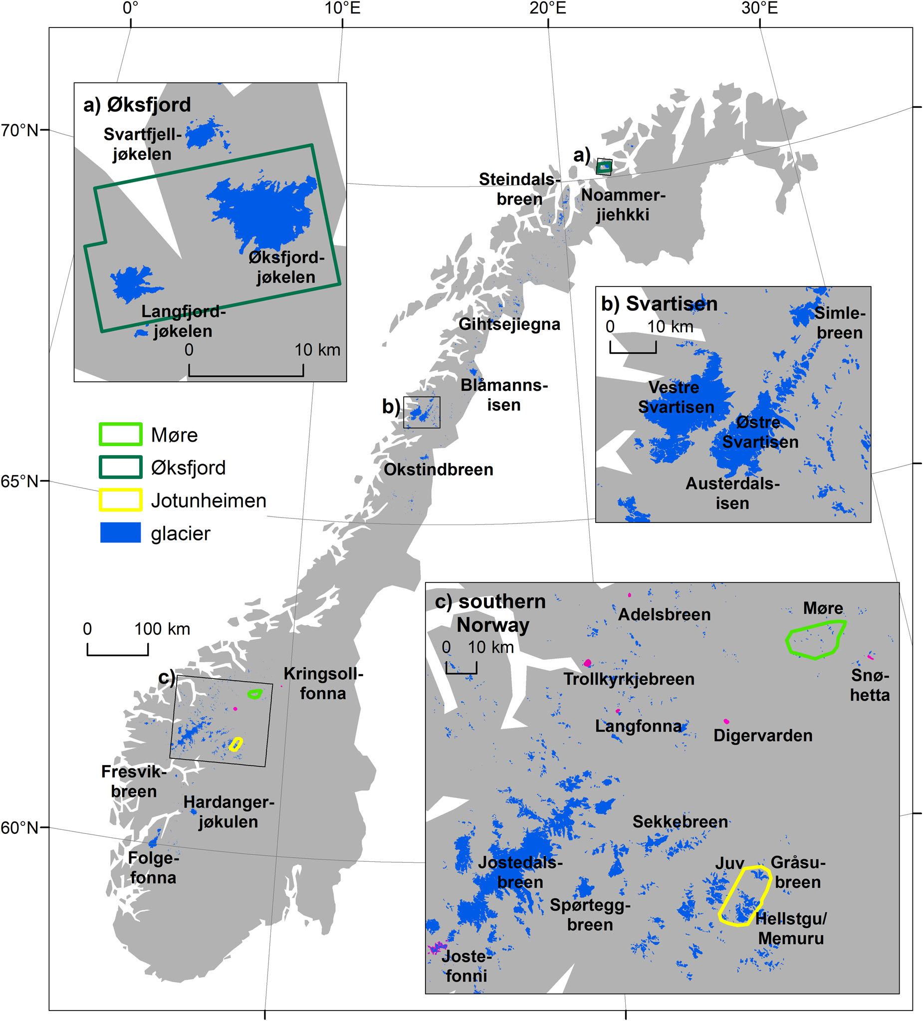
Fig. 1. Map of glaciers in Norway with names of many of the glaciers mentioned and extents of validation subsets referred to in this work. Pink colour shows the location of some of the smaller glaciers. Insets (a) Øksfjord, (b) Svartisen and (c) close up of some of the glaciers in southern Norway.
3. Data
3.1. Sentinel-2 scenes
The scenes used for glacier mapping are ideally acquired over a short time interval and have minimal seasonal snow and cloud cover (e.g. Raup and Khalsa, Reference Raup and Khalsa2007; Racoviteanu and others, Reference Racoviteanu, Paul, Raup, Khalsa and Armstrong2009). In the first years of the Sentinel era, 2015–2017, conditions were not optimal for glacier mapping in Norway due to too much snow. Scenes from August/September 2018 for northern Norway and August 2019 for southern Norway (Table S1) have less snow and cloud cover and were therefore used in this study. In total, 39 scenes were used: 34 of them were used for automatic mapping, and five were used for visual inspection (e.g. for small edits, but not used to automatically derive outlines). For some regions, multiple scenes had to be combined due to clouds obscuring the glaciers. For southern Norway, most of the scenes were taken from 27 August 2019, whereas scenes from 4 and 15 August 2019 were additionally used when glaciers were covered in clouds (Fig. 2). Earlier in the season, scenes had more seasonal snow, but had less terrain-induced shadowing due to the higher sun angle (e.g. Nagy and Andreassen, Reference Nagy and Andreassen2019). For northern Norway, most of the scenes were taken on 1 and 8 September 2018. Additional imagery from August 2019 and August/September 2018 was used when cloud coverage was unfavourable in the primary images. The glacier outline metadata describe data sources and dates used for the glaciers. In some cases, orthophotos were used due to clouds or severe terrain shadowing.
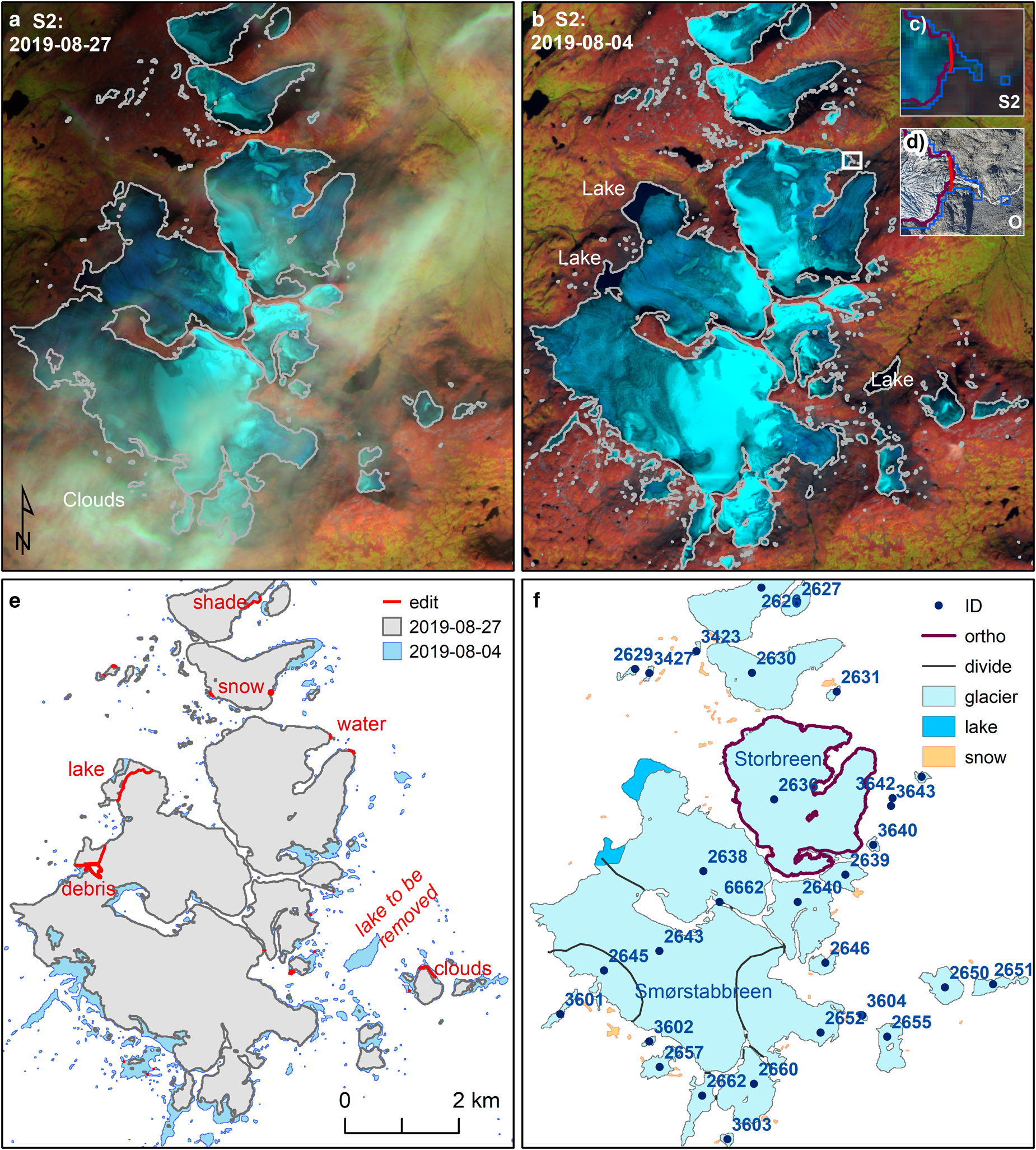
Fig. 2. Sentinel-2 images (false 11-8-4) of (a) 27 August and (b) 4 August 2019 and automatically derived outlines (grey and blue respectively). Due to cloud cover both scenes were used to derive glacier and glacier lake outlines. (c) Part of the Storbreen tongue where both a river and ice blocks had to be removed using manual line edits. (d) Orthophoto of 26 August 2019 used to manually digitise the glacier polygon (ortho). (e) Automatic mapping result shown with line edits. (f) Final results of classified glaciers and snow, ID points and ice divides. /Copernicus Sentinel data 2019/.
The Sentinel-2 scenes were downloaded as orthorectified scenes from the Norwegian National Ground Segment for Satellite Data (available at [satellittdata.no]). The orthorectified images are referred to as DTERRENG digital terrain model (DTM) data and are orthorectified using the national 10 m DTM of Norway. Geolocation errors are found in imagery orthorectified with the Planet DEM at the 90 m resolution for mainland Norway (e.g. Kääb and others, Reference Kääb2016; Andreassen and others, Reference Andreassen2021). Images orthorectified with the 10 m DTERRENG DTM were therefore preferred. Sentinel images are typically displayed in red-green-blue (RGB) colour composites of three bands or as single bands. Composite images were created using five of the bands: blue (2), green (3), red (4), NIR (8) and SWIR (11). All the five composite bands are available at a 10 m resolution, except for band 11 that is originally available at a 20 m resolution but was resampled to 10 m resolution.
3.2. Orthophotos
Orthophotos (the most recent at the time of viewing) from the Norwegian mapping authorities were used directly as web map service (wms) within the GIS and additional orthophotos were viewed in www.norgeibilder.no. The photographs were used to control the result, and to check for ice content and the extent of smaller objects that were automatically mapped from the Sentinel-2 imagery. Orthophotos originated from many different dates. Photographs taken several years prior to the Sentinel-2 scene used could not be used to directly control for glacier extent in 2018–19, as many glaciers have retreated in recent years (Andreassen and others, Reference Andreassen, Elvehøy, Kjøllmoen and Belart2020b; Kjøllmoen and others, Reference Kjøllmoen, Andreassen, Elvehøy and Melvold2021).
For some regions (Folgefonna, Hardangerjøkulen, Hardangervidda and Møre), new orthophotos from 2019 were available, the same year as the Sentinel-2 scenes used for the glacier mapping. Selected photos were downloaded and used for direct validation (Section 4.5). Snow conditions around the glaciers and the glacier extents vary during the summer as melting progresses or snowfall occurs. Whereas the 2019 Møre orthophotos were taken on the same day as the Sentinel-2 image and could be used for direct validation, most of the other 2019 photos were taken in late September after snow falls covered much of the glacier surfaces and perimeters making the orthophotos less informative (Fig. 3). For other regions, such as Jostedalsbreen, Breheimen and Jotunheimen, the most recent images were from 2015 or 2017 where snow conditions were often adverse with much seasonal snow (Fig. 3). For Fresvikbreen, the most recent images were from 19 July 2017 and had poor contrast and considerable seasonal snow cover (Fig. S1). Earlier images from 27 September 2010 were taken in a year with high melting and little seasonal snow remaining, but unfortunately a snowfall covered the surface prior to the time of the photograph being taken. For this glacier, the 19 September 2006 orthophoto provided the most information to assess ice content and glacier features. Such out-of-date images with good mapping conditions could still be useful to check the Sentinel-2 outlines in the accumulation regions with shadow, bergschrund and for the overall topography.
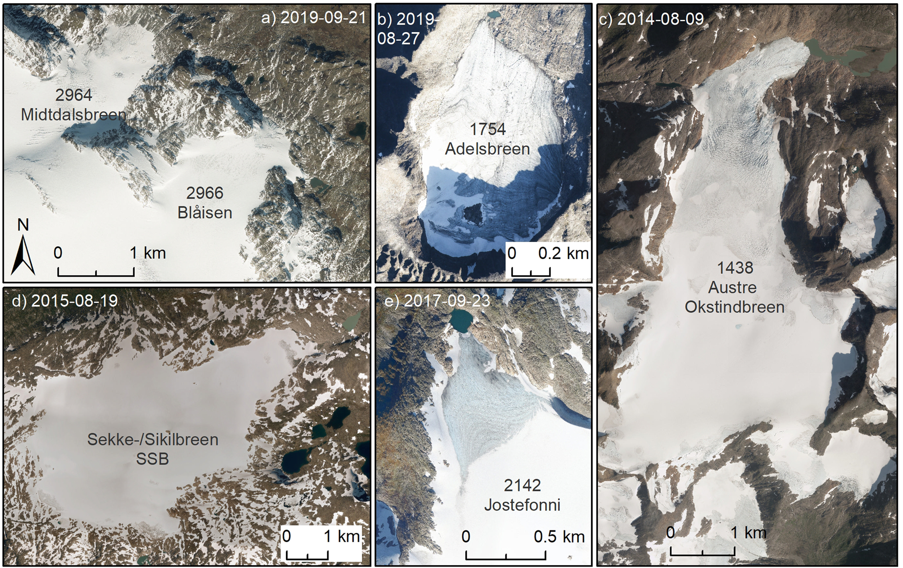
Fig. 3. Snow conditions and time of mapping varied greatly in the recent orthophotos from www.norgeibilder.no that were used to check the results from the Sentinel-2 mapping. (a) Part of the Hardangerjøkulen photo taken 25 days after the Sentinel-2 scene, glaciers are covered by fresh snow. (b) Adelsbreen, Møre, photo taken on the same day as the Sentinel-2 scene. (c) Part of Okstindbreen, photo taken 4 years earlier than the Sentinel-2 scene, (d) Sekkebreen, photo taken in 2015, a year with much seasonal snow remaining in southern Norway. (e) Part of Jostefonni, 2 years prior to the Sentinel-2 scene, seasonal snow still covered the glacier perimeter. All images © Norgeibilder.no. See Table S2.
We also had orthophotos with a 0.25 m resolution from targeted glacier surveys of Jotunheimen taken on 26 August 2019 for the Norwegian Water Resources and Energy Directorate (NVE). This survey was conducted one day before the Sentinel-2 scene of 27 August 2019 that was used to map most of the glaciers in this region.
3.3. Other datasets
Other datasets we used were:
• Satellite orthoimages derived from Pléiades scenes (© CNES 2019, Distribution Airbus DS). The two scenes we used were acquired near the time of the Sentinel-2 scenes used for the glacier mapping and were therefore optimal for validation of the outlines. One scene covered Øksfjordjøkelen and Langfjordjøkelen and was acquired 1 September 2018. The other scene covered parts of Jotunheimen and was acquired 27 August 2019. The scenes were available in 0.5 m (panchromatic) and 2 m (multispectral) resolution.
• The 10 m national DTM from the Norwegian mapping authorities.
• Standard topographical data of Norway (administrative borders, lake, land cover, elevation contours, etc.) as vector layers and as wms from the Norwegian mapping authorities.
• NVE's glacier inventory from 1999 to 2006 including over 400 PSF polygons without glacier ID (Andreassen and others, Reference Andreassen, Winsvold, Paul and Hausberg2012).
• NVE's glacier lake inventories from 1999 to 2006, 2014 and 2018 (described in Andreassen and others, Reference Andreassen2021 and references therein).
4. Methods
4.1. Glacier delineation
To map the ice bodies, we applied a standard band ratio method with a threshold on the selected Sentinel-2 scenes. This method uses threshold values and should be optimized for each satellite scene; however, the optimum threshold can be difficult to find and can vary also within a scene (Paul and others, Reference Paul, Winsvold, Kääb, Nagler and Schwaizer2016). Two thresholds were used. A band ratio threshold (T1) was calculated as the red band 4 divided by the shortwave infrared band 11 (SWIR). A threshold in the blue band 2 (T2) was used to improve classification in shadow (Paul and Kääb, Reference Paul and Kääb2005; Paul and Andreassen, Reference Paul and Andreassen2009; Winsvold and others, Reference Winsvold, Andreassen and Kienholz2014; Paul and others, Reference Paul2020). A median filter of 3 × 3 pixels kernel (30 × 30 m) was thereafter applied to reduce noise in shadow and remove isolated pixels. Then the selected thresholded result was converted to polygons. We incremented the band ratio and band thresholds with steps of 0.2 and 50, respectively, to find an optimal combination (Fig. 4). To include the dirty ice around glacier perimeters, T1 should be kept as low as possible (Paul and others, Reference Paul2013). Some of the smallest glaciers or possible snow fields may not be mapped for large values of T1 and T2 (Winsvold and others, Reference Winsvold, Andreassen and Kienholz2014). In our study, selected values of T1 varied between 2.0 and 3.0 and selected values of T2 varied between 1000 and 1200 (Table S1). In Jotunheimen, we chose a low value of T2 (1000) so as to not underestimate the shadowed parts (Fig. 4). For debris-free ice, the result was not very sensitive to the thresholds chosen (Fig. 4). Generally, less ice is mapped with a large band ratio threshold. The results were checked glacier-by-glacier using the orthophotos and Sentinel composites of natural colour (4-3-2), false colour composites (8-4-3 and 11-8-4) and single bands. Band 2 was useful for parts in shadow. Geolocation errors were found in some of the orthophotos. The Sentinel-2 scenes were in any case the primary source for the glacier and glacier lake outlines. Therefore, when editing and checking the datasets, the Sentinel-2 images were preferred as a background for consistency, whereas the orthophotos were used for familiarising oneself with the region and cross-checking (potential) ice content. Topographic maps were used as both wms and vector layers for identifying new glacier names and general topography (Fig. 5). The lake and land vector data of Norway were used to remove water bodies that were included in the automated mapping.
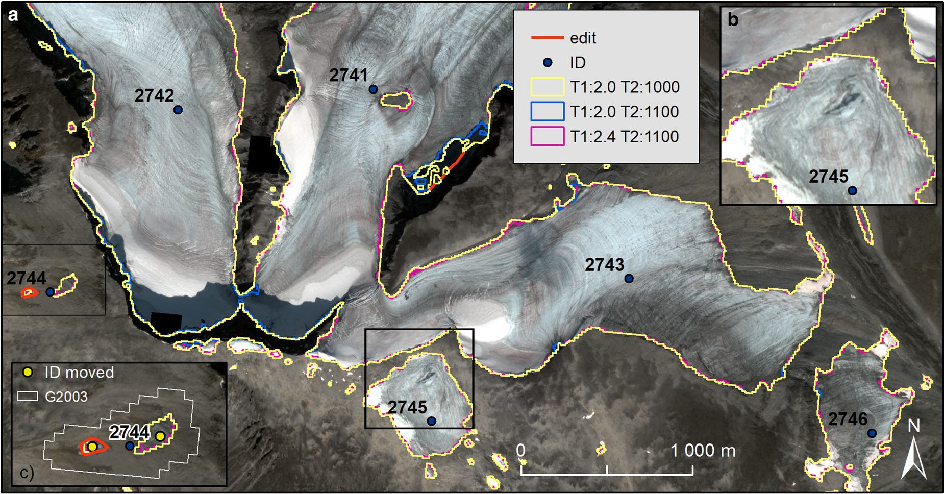
Fig. 4. (a) Three automatically derived outlines with values of T1 and T2 for a subset of Grjotbrean (2742 + 2741) and Gråsubreen (2743) in Jotunheimen from a Sentinel-2 scene from 27 August 2019 compared with a Pléiades image of the same date. (b) Detailed part of Glitterbrean and Gråsubreen. There is no difference between T2 1100 and 1000 in this part. (c) A small ice patch (ID 2744) that disintegrated since 2003 and where the ID was moved. The smallest part was manually edited in this case. The T1: 2.0 and T2:1000 were used as the final outline with edits. Many of the smaller polygons were not included in the final inveentory. /Pléiades © CNES 2019, Distribution Airbus DS.2019/.
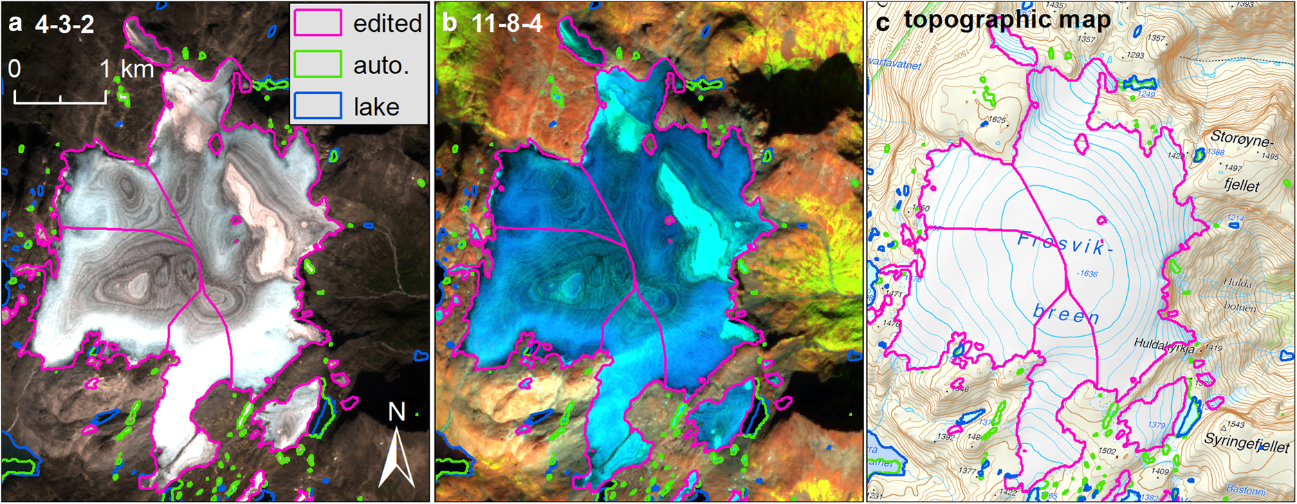
Fig. 5. (a) Sentinel-2 scene from 27 August 2019 for Fresvikbreen displayed in natural colours (band 4-3-2) and (b) false colours (band 11-8-4), with automatically (auto.) derived outlines and edited outlines (removal of lakes and snow and other edits). Lake: lake layer from the topographical main map series of Norway (N50). (c) The topographic map as wms from the Norwegian mapping authorities was used to check glacier names and topography. For Fresvikbreen orthophotos from 2017 (extensive snow cover), 2010 (fresh snow) and 2006 (minimal snow) from © Norgeibilder.no were also checked (Fig. S1). /Copernicus Sentinel data 2019/.
Where edits were needed, these were digitised as line segments and an edit code was associated with the line segment. The line segment was used to modify or cut the polygon. In this way, it was possible to track the edits that were made (Fig. 2).
Manual corrections are typically needed for water bodies, debris cover, shadow, snowfields and ice on water (e.g. Paul and others, Reference Paul and Andreassen2009). As in the previous 1999–2006 inventory, the main corrections were inclusion of shaded areas and editing at the glacier-lake interface (Andreassen and others, Reference Andreassen, Winsvold, Paul and Hausberg2012). Most glacier regions across Norway have little supraglacial debris. However, in areas of steep terrain (e.g. Lyngen, Jotunheimen, Møre and Sunndal which are dominated by small cirque and valley glaciers), supraglacial debris is more prominent and some debris-covered parts were corrected using manual digitisation. Moreover, automatically mapped holes (nunataks) were closed when they were likely to be debris. This was difficult to judge from the Sentinel-2 images alone, so uncertainties remain for smaller nunataks. It was also difficult to control parts in heavy terrain shadow, which also may include debris cover. Images captured earlier in the year (e.g. early summer) proved useful in determining areas prone to heavy shading, but determining glacier extent remained challenging where debris cover was present. Such debris-covered extents will have larger uncertainties. Seasonal snow was, as in previous inventories of Norway, a challenge especially along the margins of a glacier where it can persist late into, and sometimes throughout, the melt season (Fig. 3). In some cases, this was cut out and marked as snow (Fig. 2) but it can be difficult to separate snow from disintegrating ice. To keep such edits to a minimum, continuous polygons were mostly kept as is.
4.2. Glacier classification
A glacier can be defined as ‘a perennial mass of ice, and possibly firn and snow, originating on the land surface by the recrystallization of snow or other forms of solid precipitation and showing evidence of past or present flow’ (Cogley and others, Reference Cogley2011). We followed the same overall structure as in the previous inventory and divided the bodies into glaciers, ice patches or snow (Andreassen and others, Reference Andreassen, Winsvold, Paul and Hausberg2012). Snow was excluded but kept in a separate layer so it could be used in other applications or reselected if needed. Thanks to the higher resolution of Sentinel-2 (10 m) over Landsat (30 m) used in the 1999–2006 inventory, smaller items could be mapped. In the 1999–2006 mapping, the lower threshold was nine pixels, equivalent to 8100 m2 (0.0081 km2). With Sentinel-2, we selected nine pixels as the initial threshold, thus only 900 m2. As glaciers are shrinking and disintegrating even such small polygons can contain ice. All bodies larger than nine pixels were inspected by at least checking the Sentinel images. Many of the smaller polygons (<4000 m2) were quickly classified as snow based on topography and elevation in the region. As smaller ice bodies are also of interest in Norway, e.g. due to archeological finds that have been numerous on many small bodies since 2006 (e.g. Nesje and others, Reference Nesje2012; Pilø and others, Reference Pilø, Barrett and Eiken2021), we decided not to have a higher threshold. A test of ten archeological sites of interest showed that small ice bodies can be mapped with reasonable accuracy using Sentinel-2 images (Andreassen and others, Reference Andreassen, Callanan, Saloranta, Kjøllmoen and Nagy2020a). Furthermore, small polygons were often indicators of glaciers or ice patches in shadow (e.g.in cirques) that were not fully detected by the algorithm. Thus, by keeping this low size threshold, we detected several smaller glaciers in shadow and manually edited them. When recent orthophotos were not available or the mapped body was totally snow covered, the classification was based on previous classification, and appearance of ice in the Sentinel-2 image. Size is often used as a criterion for defining an ice body as a glacier, but some very small bodies in steep terrain can have ice content and crevasses. On the other hand, snow bodies can be large and have no ice content, but snow patches in steep terrain may have snow crevasses due to gravity.
Leigh and others (Reference Leigh2019) used Landsat imagery and orthophotos from norgeibilder.no to map glaciers in glacier regions 2 (Øksfjord) and 3 (Troms – North) (Andreassen and others, Reference Andreassen, Winsvold, Paul and Hausberg2012). They proposed a scoring system that can be used to classify glaciers in categories as certain, probable, possible and perennial snow. Scores of 1–5 points (maximum 20 in total) are given based on the appearance of crevasses, flow features, ice, etc. (Table S3). For example, a body with crevasses, deformation features and visible areas of ice will score >10 points and be classified as ‘certain’. A body that has ice and features indicating past flow will score as a ‘probable’ glacier and be classified as an ice patch or ice remnant. A body of ice with no presence of flow features or deformation will be categorized as ‘possible’. The advantage of this method is that it can be used objectively to categorize mapped bodies. The disadvantages are that it requires recent orthophotos and is a manual and time-consuming method. It is also difficult to differ between perennial and seasonal snow, as few of the orthophotos are taken at the end of the season (Fig. 3). In our study, we tested the scoring principles by Leigh and others (Reference Leigh2019) in a subregion (see Section 6.1). We also leaned on the classification criteria to aid the assignment, without assigning individual scoring points to each body.
4.3. Glacier attributes
For comparison purposes, we decided to use the ice divides from 1999 to 2006 as far as possible. Glacier divides were updated for some glaciers to fit with divides used in NVE's mass-balance calculations (Fig. S2). Some other minor edits were carried out, mainly to separate units more naturally. On many of the smaller glaciers, the 1999–2006 ice divides were not needed for the 2018–19 dataset due to glacier shrinkage or the fact that the Sentinel-2 resolution of 10 m was much better at separating neighbouring glaciers compared to the 30 m Landsat resolution. Glacier ID points were kept as is but moved if they were no longer within the glacier polygon or close to the polygon border due to glacier shrinkage. In cases where the glacier had disintegrated to several parts, the point was moved to the largest remnant or most ‘glacier-like’ remnant (Fig. 4c). This was done using topology editing and manual inspection in the GIS (©ArcMap 6.1). Each polygon was assigned a unique ID for 2018–19 that was either new or inherited from 1999 to 2006. All polygons within the 1999–2006 glacier extent inherited the 1999–2006 glacier ID as a secondary ID. In this way, one can calculate observed changes and have a unique identifier.
4.4. Glacier lakes
The semi-automated method used for glacier outline mapping in our study often requires manual edits to detach glacier lakes connected to the glacier outlines (Fig. 2). Thus, we produced an updated glacier lake outline dataset for 2018–19 to match the new 2018–19 glacier outlines. We included additional lakes for glaciers smaller than the 0.25 km2 threshold for glacier size that was set for the 2018 product (Nagy and Andreassen, Reference Nagy and Andreassen2019). For northern Norway, the glacier lakes were used as in the 2018 product, with some corrections and additions of lakes at glaciers below the 0.25 km2 glacier size threshold. The Sentinel-2 scenes used for the 2018 mapping were taken earlier in the season than the glacier outline mapping. This had the advantage of less terrain shadows but the disadvantage of more snow and ice remnants at the glacier perimeter and lake surface.
For southern Norway, we updated and mapped the lakes using the 2019 imagery. The glacier outline-lake interface was manually digitized as a line based on the Sentinel-2 imagery used for the glacier outline mapping. Each digitized lake interface line was given an edit code for ‘glacier lake’, and the glacier lake was detached from the glacier by splitting the mapped polygon with the digitized line. This often resulted in a polygon partly covering the glacier lake. To map the full glacier lake extent, the automatically mapped glacier lakes were either modified, extended with manual edits or merged with the 2018 outlines or lakes from the topographic map series 1:50 000 of Norway. Orthophotos from norgeibilder.no or other Sentinel-2 imagery were used to verify glacier lakes where newer photos were available, however not all lakes could be verified due to snow conditions, lake ice, or lack of recent orthophotos. For some of the smaller glacier lakes, the outline was automatically mapped and used ‘as is’ after splitting, while other parts of the lakes were manually digitized. Supraglacial lakes were also manually digitized. Large lakes were often easy to detect, while small and newly formed lakes were more difficult to identify and thus more uncertain. The lakes appeared dark in false colour composites compared to snow and ice, but very small glacier lakes were difficult to differentiate from debris, shadow or braided rivers. Lake colour also varied due to sediment content and lake size and shape (e.g. Matta and others, Reference Matta, Giardino, Boggero and Bresciani2017; Nagy and Andreassen, Reference Nagy and Andreassen2019). For this lake inventory, we included lakes that were likely to be in contact with the glaciers at the time of satellite image acquisition.
4.5. Validation
To validate our Sentinel-2 semi-automated mapping, we compared our data with manual digitisation from aerial orthophotos of selected glaciers in Jotunheimen, Møre, Dovre and Hardangerjøkulen (0.25 m resolution) and Pléiades orthoimages (0.5–2 m resolution) available for a subset in Jotunheimen and Finnmark. Below, we describe five validation cases. The manual digitisation described here was done independently of the Sentinel-2 mapping. An orthophoto or orthoimage was the only product available for the digitiser except for Langfjordjøkelen (case 4.5.1). Results from the validation and other sensitivity tests are summarized in Table 7 in Section 6.3.
4.5.1. Pléiades orthoimage and aerial orthophotos for a subset of Jotunheimen
In the first evaluation, a subset of the Pléiades scene of 27 August 2019 (0.5 and 2 m orthoimage) was used. The scene was acquired the same day as a Sentinel-2 scene used for the glacier mapping. Two of the authors independently digitised the glaciers manually. These were then compared with the final Sentinel-2 outlines for a total of 49 glaciers or ice bodies ranging from 0.002 to 8.1 km2 in area (Figs 4, 6–8). Some of the glaciers were mapped as two bodies in the Pléiades digitising, and one body by the Sentinel-2 algorithm (Fig. 7b). We compared the area sum of the bodies, and results revealed that the mapped glaciers differed between the two authors. Some smaller bodies were mapped by one author only. Some of the bodies were not included in the Sentinel mapping. The total area of the mapped ice bodies by the two authors using Pléiades was 40.95 and 40.52 km2, respectively, while the results from using Sentinel-2 was 40.63 km2. Thus, the Sentinel-2 area was 0.28% smaller or 0.78% larger compared to Pléiades reference. It is noteworthy that the Sentinel-2 estimate lies between those from Pléiades and that the Pléiades estimates for individual glaciers have larger variations (Fig. 6).
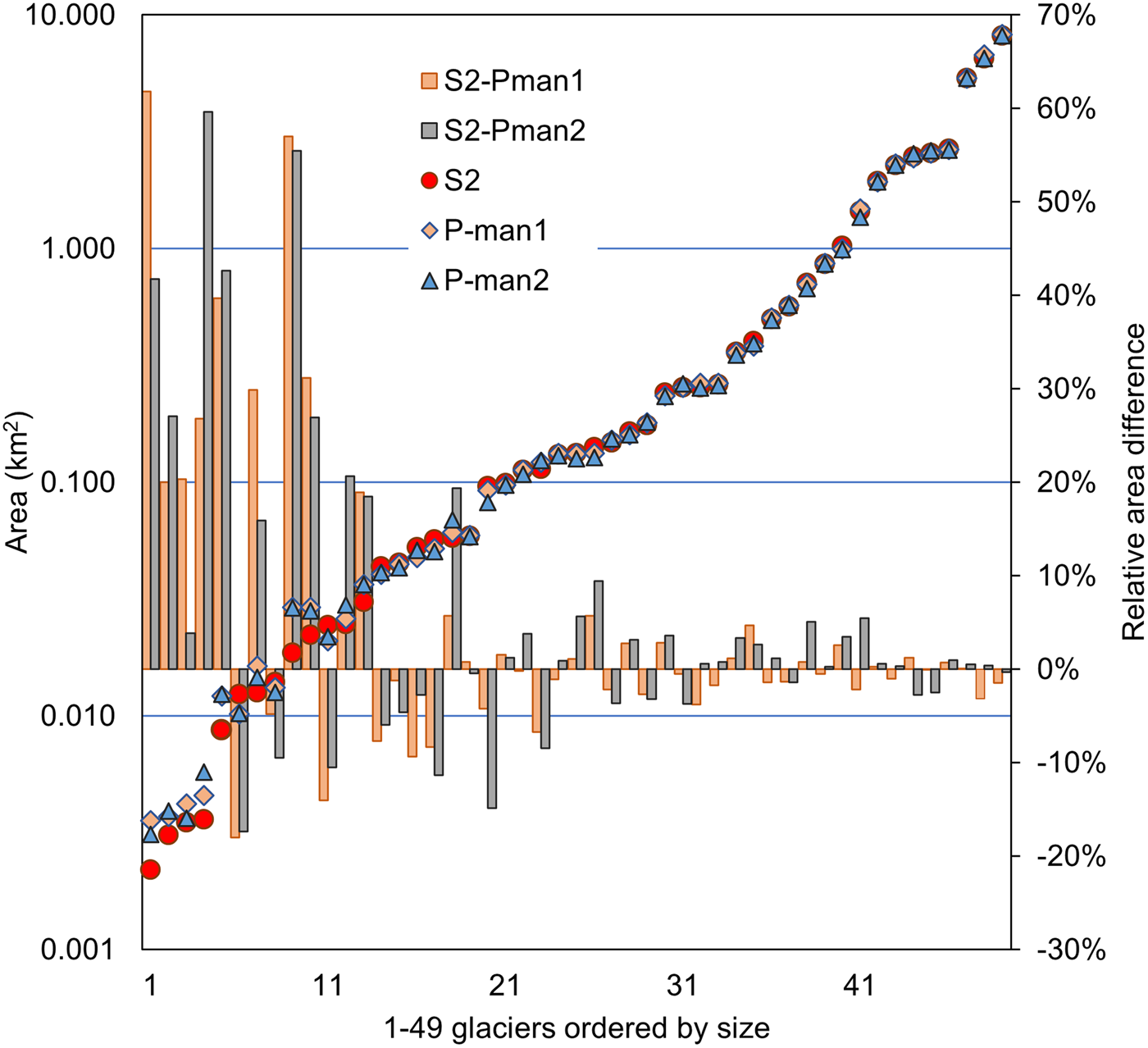
Fig. 6. Area derived from Sentinel-2 (S2) vs two independent manual digitisations from Pléiades imagery (P-man1 and P-man2) for a subset of 49 glaciers in Jotunheimen. Relative area differences are also shown. See Figures 4, 7 and 8 displaying some of the glaciers. Note that the scale is logarithmic on absolute left y-axis.
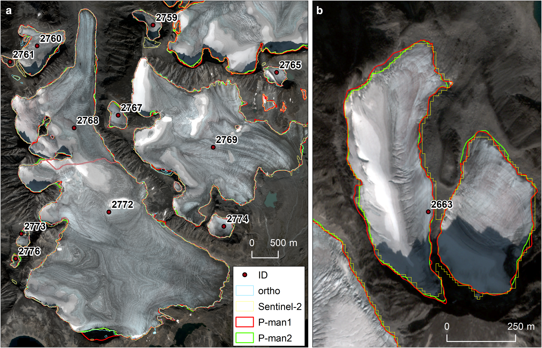
Fig. 7. Subset of the Pléiades scene of 27 August 2019 showing (a) Hellstugubreen (2768) and surrounding glaciers, and (b) glacier ID 2663. Figure 7a has one more outline (ortho), derived from orthophotos from 26 August 2019. /Pléiades © CNES 2019, Distribution Airbus DS/.
For a selection of glaciers in the Pléiades subset we had orthophotos taken on 26 August 2019 (0.25 m resolution), the day before the Sentinel-2 and Pléiades imagery. These glaciers were digitised by two of the authors (one digitisation per glacier). In total, 15 smaller and larger ice bodies were mapped, ranging in size from 0.01 to 8.16 km2. The total glacier area derived from the orthophotos was 19.59 km2, whereas the total glacial area derived from the Sentinel-2 was 19.53 km2, which represents a 0.3% difference. Of the ten glaciers in the sample larger than 0.1 (0.3) km2, amounting to 99 (96) % of the area, the relative differences were within ±4%. The glaciers smaller than 0.1 km2 had relative differences ranging between −66% (for the smallest glacier) and 9%. The three datasets (Pléiades, Sentinel-2 and aerial orthophotos) were taken with a 1-day time difference and melting along the perimeter is considered negligible. Results for Gråsusnippen (ID 2746), a 0.4 km2 ice patch, revealed that manual digitization attempts between the two authors differed by 2–5%. Differences were mainly due to decisions by the observer on what to include in the perimeter (Fig. 8). Using 2.4 as threshold T1 instead of 2.0 would reduce the area by 0.016 km2, or 4%. The area of Gråsusnippen ranges between 0.401 and 0.382 km2 for the various methods and rounds to 0.4 when using one decimal.
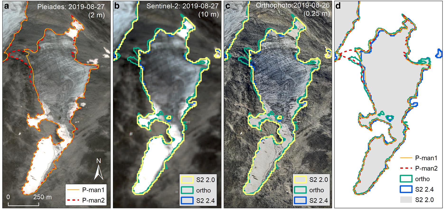
Fig. 8. Gråsusnippen (ID 2746) as mapped by manual digitisation of Pléiades image (P-man1 and P-man2), semiautomatic from Sentinel-2 (S2 2.0 and 2.4) and manual from orthophoto (ortho) together with resulting outlines. Here the largest difference is in the interpretation of dark ice in the north-western part. (a)Pléiades image, (b) Sentinel-2 (natural 4-3-2), (c) Orthophoto and (d) resulting outlines. /Pléiades © CNES 2019, Distribution Airbus DS. /Copernicus Sentinel data 2019/.
4.5.2. Glaciers around Snøhetta, Dovre
Three glaciers around the Snøhetta peak (Dovre, Innlandet county) were digitised by one author using orthophotos from 27 August 2019 from norgeibilder.no, the same day as the Sentinel-2 scene. The Sentinel-2 outlines were edited in areas of terrain shadow and at the terminus of one glacier (Fig. 9). The terrain shadowing and supraglacial debris made mapping in this region challenging. Some parts were corrected when cross-checking with the orthoimage and Sentinel-2 image. The total area of the three glaciers was 1.53 km2 for the orthophoto, 1.50 km2 for the Sentinel-2-edited and 1.40 km2 for the automatically derived product (Table 1). In the Snøhetta case, the automatic mapping resulted in the smallest areas, as parts in shadow were not mapped. The manually digitised outline from the orthophotos gave a 2.0% larger area than the corrected Sentinel-2, and a 9.5% larger area than the automatically derived outline. This illustrates how glacier areas can be underestimated in shaded or debris-covered parts.
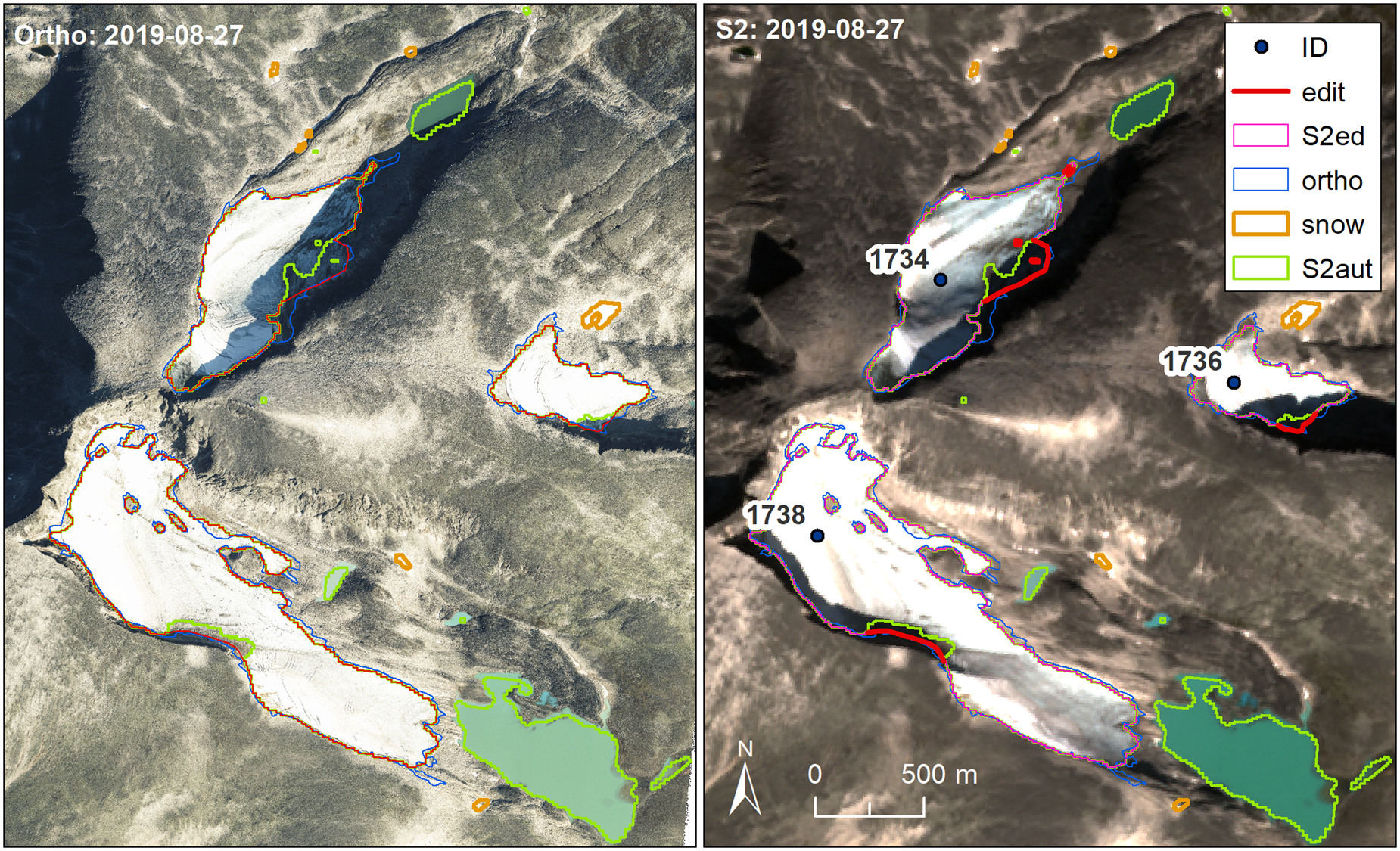
Fig. 9. Glaciers at Snøhetta as mapped from orthophotos and Sentinel on the same day, 27 August 2019. Left: orthophoto from norgeibilder.no. Right: Sentinel-2 image. Edit, manual edits; S2ed, Sentinel-2 with manual edits; ortho, manual digitised from orthophoto; snow, polygons classified as snow; S2aut, automatic outline classified from Sentinel-2. Note that the lakes are included in the automatic mapping. None of the lakes are now connected to the glacier. See Figure 1 for location. /Copernicus Sentinel data 2019/© Norgeibilder.no/.
Table 1. Resulting areas (A) of automatic mapping of Sentinel-2 (S2or), edited mapping (S2ed) and manually digitised from orthophoto (Ortho) and relative area differences ΔA between S2ed or S2or and Ortho (O), for the Snøhetta glaciers
4.5.3. Ice patch at Digervarden
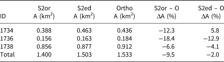
The Digervarden ice patch is of interest due to an archaeological ski find in 2014 (Finstad and others, Reference Finstad, Martinsen, Hole and Pilø2018). The ice patch was mapped with Landsat for the 1999–2006 inventory but was only included in the PSF layer stored in the NVE database (Fig. 10). The area mapped from the Landsat image taken on 9 August 2003 was 0.173 km2, whereas the area of the five ice bodies automatically mapped using Sentinel-2 from 27 August 2019 was 0.055 km2. A comparison of Sentinel-2 derived outlines with orthophotos from the same date revealed that the automatic mapping algorithm did not always capture the full perimeter along very thin and dark ice (typically remnants of ice and disintegrating parts) (Fig. 10). The manually digitized outlines from orthophotos (Fig. 10) resulted in a larger total area of 0.076 km2. The area of the two smaller items not included in Sentinel-2 mapping was 0.006 km2. They were also detected by the automatic mapping but were not included due to their insufficient size of four pixels. The total area of the present ice patch parts was 0.021 km2, 38%, larger than as mapped with Sentinel-2. Our Sentinel-2 mapping did not capture all parts of small bodies with dark surfaces. In detailed studies of such bodies, it is possible to manually digitize more ice from the Sentinel-2 images or fine-tune the thresholds.
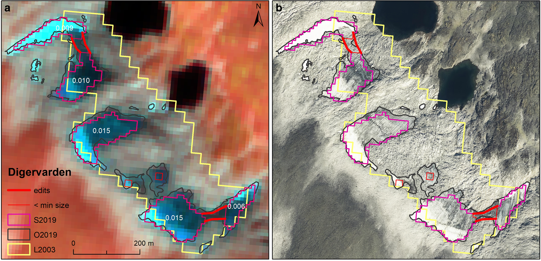
Fig. 10. Small ice patches mapped from Sentinel-2 (S2019) at Digervarden, Lesja, Innlandet county, compared to independent manual digitization from orthophotos taken the same day (O2019). (a) Sentinel-image from 27 August 2019 (false 11-8-4). (b) Orthophoto from the same day. The ice patches were mapped as one body (L2003) in the 1999–2006 inventory, and there included as a possible snowfield layer without any assigned ID./Copernicus Sentinel data 2019/© norgeibilder.no/.
For 2018–19, we selected one T1 and T2 threshold per scene ranging from 2.0 to 3.4 for T1 and 1000 to 1200 for T2 (Table S1), whereas the optimal threshold will vary through the scene (Paul and others, Reference Paul, Winsvold, Kääb, Nagler and Schwaizer2016). In this case, the orthophoto was the best source for a detailed outline, but Sentinel-2 has the advantage of a much higher temporal coverage, allowing us to follow the seasonal and annual changes (Andreassen and others, Reference Andreassen, Callanan, Saloranta, Kjøllmoen and Nagy2020a). In our overall manual edits, we added more ice in some cases (Fig. 4; inset 2744). However, in many cases, we did not have such validation data, and to obtain a consistent dataset and reduce the manual edits, we did not overedit such parts. Although the percentage differences may have been large, the excluded parts only contributed to a small area and ice volume.
4.5.4. Glacier and glacier lake Langfonna and Hardangerjøkulen
We also tested our semi-automated lake mapping with manual digitisation by two of the authors for two sites (Fig. 11). At Langfonna glacier (ID1864) in Møre og Romsdal, the lake area of the Sentinel-2 scene from 15 August (0.235 km2) coincided within ±1% of the digitisation from orthophotos (0.232 and 0.234 km2) from 27 August 2019 (Table 2). For the glacier area, the difference was larger. The Sentinel-2 area was 0.374 km2 and the manual digitisation was 0.348–0.360 km2. This corresponds to a 4–7% smaller area, which was mainly due to less snow being included and less glacier area mapped in the steep part on the eastern rim. Some of the difference may also have been due to snow melting between 15 and 27 August 2019 (the image of 27 August 2019 had clouds and was not used).
Fig. 11. (a) Glacier lakes Langfonna, Møre. (b) Glacier lakes at western part of Hardangerjøkulen (HAJ). See Figure 1 for location. Orthophotos from © norgeibilder.no are from (a) 27 August and (b) 26 July (left part) and 21 September 2019 (note the fresh snow).
Table 2. Lake area derived for a lake at Langfonna and several lakes at Hardangerjøkulen
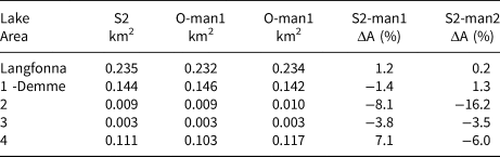
S2: lake area mapped from Sentinel-2. O-man1 and O-man2: digitised manually from orthophotos. S2-man1 and S2-man2: differences (percentage) between lake areas derived from Sentinel-2 and from orthophotos. See Figure 11.
An additional test was carried out by digitising the glacier-dammed lake Demmevatnet at the outlet glacier Rembesdalskåka and three other ice-marginal lakes in the western part of Hardangerjøkulen (Fig. 11b). Here, the area of lake Demmevatnet was within 1% of the Sentinel-2 derived lake areas, whereas the three other lakes varied between 3 and 16%. Demmevatnet was drained in a GLOF event on 24 August 2019 and was thus empty at the time of mapping the glacier outline and lakes 2–4 (Fig. S3). Therefore, the earlier image from 4 August was used for Demmevatnet (Fig. S3). The largest relative area difference was for the smallest lake in the sample (lake 2). The largest difference in absolute area was for lake 4, with differences of −0.007 and 0.008 km2. Floating ice was included in one of the manual digitisations from orthophoto but excluded in the other manual and in the Sentinel-2 manual correction. In cases with floating ice or ice bergs close to the ice-lake interface, the lake outline was more uncertain.
Our testing revealed that glacier lakes can be mapped accurately from Sentinel-2 using our semi-automated approach. The lakes are clearly visible and easy to detect once they reach a size of ~0.1 km2, but smaller lakes are more uncertain. Based on our experience using NDVI and manual digitization on the Sentinel-2 image, the accuracy in manual mapping or semi-automated mapping as used here is as good as or better than the automatic approaches and can be faster, at least for a region such as mainland Norway.
4.5.5. Glacier extents of Øksfjordjøkelen and Langfjordjøkelen
Pléiades images available for two ice caps in Finnmark, Øksfjordjøkelen and Langfjordjøkelen were used to digitise the glacier outlines (one outline per glacier). The resulting area derived from manually digitised outlines was 35.9 km2 for Øksfjordjøkelen and 6.2 km2 for Langfjordjøkelen, while the results from the semi-automated mapping were 36.3 and 6.4 km2, respectively (Fig. 12, Fig. S4). It should be noted that for the Sentinel-2 imagery-based outlines for Landfjordjøkelen, the Pléiades images and outlines were compared when deciding the T1 and T2-values and as such, these outlines are not independent. The area difference between Pléiades and Sentinel-2 for Øksfjordjøkelen and Langfordjøkelen of 1.2% (0.44 km2) and 3.1% (0.20 km2), respectively, point to what can be expected when mapping Norwegian ice caps with relatively clean ice but with some shadow issues.
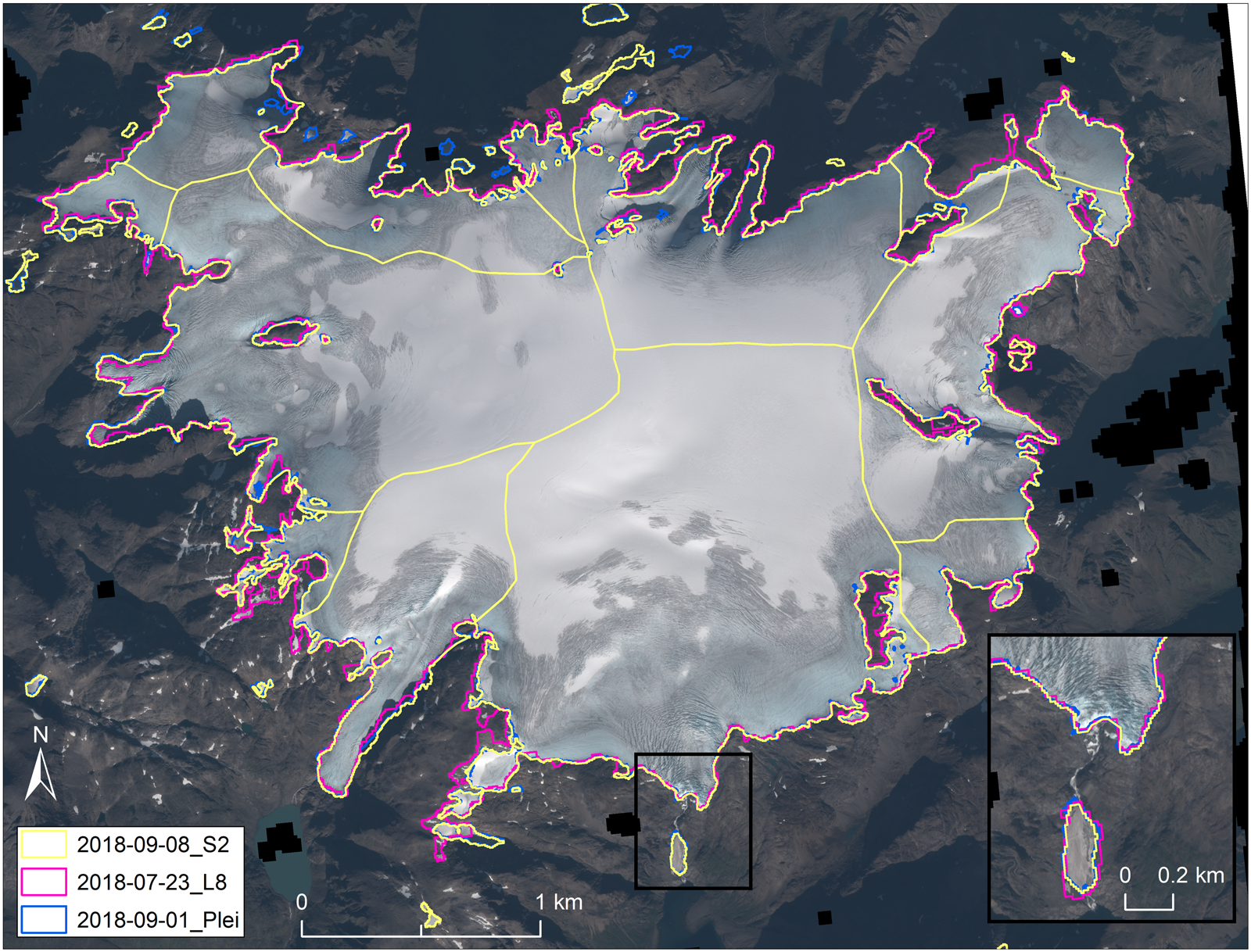
Fig. 12. Øksfjordjøkelen in Finnmark mapped manually from Pléiades orthoimage and semi-automatically from Sentinel-2 and Landsat 8 images from 2018. Inset shows the lower part of the outlet Isfjordjøkelen (ID 47) and the regenerated glacier Nerisen (ID 48). Background is Pléiades image shown in colour at 2 m resolution. The black pixels represent unmatched areas in the orthoimage. /Pléiades © CNES 2019, Distribution Airbus DS/.
5. Results
5.1. Total area and number of glaciers
The total area of glaciers mapped in the new 2018–19 inventory of Norway is 2328.4 km2. This includes 2375 ‘newly’ mapped ice bodies totalling 48 km2. The ‘new’ bodies range in size from <0.001 to 0.205 km2 and 23 of them are larger than 0.1 km2. When excluding those mapped as PSF in 1999–2006 (e.g. Digervarden, Fig. 10), there are still over 2000 ‘new’ bodies totalling 37 km2 with nine larger than 0.01 km2. Mapped snow polygons not included in the 2018–19 inventory represented an area of 98 km2 in total. Glaciers with a size of >5 km2 (>1 km2) >0.5 km2 amount to 46% (78%) 85% of the total area. Glaciers and ice bodies smaller than 0.1 km2 amount to 5.6% of total area and 75% of the total number. A total of 60% (1399.9 km2) of the glacier area is in southern Norway and 40% (928.5 km2) is in northern Norway (Table 3). For the ten largest glacier complexes (glaciers not divided into glacier units), the total area is 1214.2 km2 in 2018–19 and they represent 52% of the total area. Glaciers in Norway are mainly found in the counties Vestland (1077 km2, 46% of total glacier area), Nordland (722 km2, 31% of total area), Innlandet (247 km2, 11% of total area) and Troms and Finnmark (207 km2, 9% of total area). These four counties contain 97% of the total area (Fig. S5). Norway and Sweden are divided into three GTN-G (RGI) subregions in glacier region 8 Scandinavia (GTN-G, 2017) (Fig. S5). The glacier region 08-01 (N Scandinavia) contains 928 km2 (40% of total Norway), 08-02 (SW Scandinavia) contains 1137 km2 (49% of total) and 08-03 (SE Scandinavia) contains 263 km2 (11% of total). Whereas the two GTN-G subregions 08-02 and 08-03 are fully covered by our inventory, the 08-01 region lacks the Swedish glacier area.
Table 3. Mapped glaciers and ice patches included in the 2018–19 inventory derived from Sentinel-2 per size class
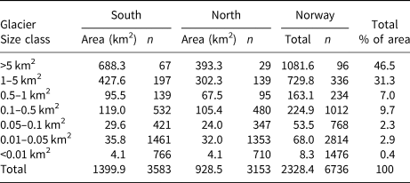
A, area; n, number. The glaciers are divided into units, e.g. Jostedalsbreen as more than 80 units.
5.2. Glacier area change from 1999–2006 to 2018–2019
The total glacier area of Norway declined from 2692 km2 in 1999–2006 to 2328 km2 in 2018–2019, which is a reduction of 364 km2, or 13.5%. Including the PSF layer mapped for 1999–2006 gives a total area of 2716 km2 and thus a reduction of 388 km2 or 14.3%. The 3143 glaciers included in 1999–2006 had a total area of 2281 km2 in 2018–2019, a reduction of 411 km2 or 15.3%. All 36 glacier regions used in the 1999–2006 inventory (Andreassen and others, Reference Andreassen, Winsvold, Paul and Hausberg2012; Winsvold and others, Reference Winsvold, Andreassen and Kienholz2014) have a reduced glacier area, with the largest losses in the northernmost regions (Fig. S6). When only considering the glaciers mapped in the 1999–2006 inventory, the glacier area in northern Norway (regions 1–19) was reduced from 1170 to 910 km2, a loss of 260 km2 or −22%. The glacier area in southern Norway (regions 20–36) was reduced from 1522 to 1371 km2, a loss of 151 km2 or −10%. The largest losses are observed in Svartisen East (55 km2), Svartisen West (39 km2) and Jotunheimen West (26 km2). It should be noted that the northern regions 4–19 have 1999–2006 mapping years 1999 and 2001, whereas the southern regions were mapped in 2002, 2003 and 2006, thus most of the changes in northern Norway are for a longer period. Looking at percentage change per year for all regions, the five regions with the most negative change per year are: 35 Hardangervidda, 18 Vefsn, 8 South Troms, 34 Hardangervidda and 32 Hallingskarvet, with changes ranging from −3.2 to −3.0% a−1. All these regions are characterised by small glaciers. The regions with the smallest negative changes are 25–27 Jostedalsbreen (South, Mid, North), 33 Hardangerjøkulen and 32 Folgefonna, with changes in the range between −0.27 and −0.62% a−1. These regions include some of the largest glaciers in Norway.
Some of the glacier complexes have parts that are now detached from the main glacier, such as Gihtsejiegna (Fig. 13b). The detached parts are not counted in the current area for the glacier complex, but as a separate unit. The detached glaciers are, however, included in the overall glacier area for Norway and in glacier change analyses. Furthermore, it should be noted that some of the disconnecting of glaciers in the new inventory is likely attributed to better spatial resolution of the Sentinel-2 imagery and availability of orthophotos as opposed to actual breakup of glaciers between the inventories. The ten largest glacier complexes have all shrunk since 1999–2006 (Table 4). When including the detached parts in the analysis to assess the overall glacier changes, a total reduction of 87 km2 or 6.6% of the ten complexes is observed. The largest relative reduction is for Okstindbreen (0.7% a−1), whereas Jostedalsbreen has been reduced the least in relative area (0.2% a−1). Some of the individual tongues of Jostedalsbreen have retreated markedly, such as Bødalsbreen (~880 m), Nigardsbreen (~650 m), Austdalsbreen (~300 m) and Tuftebreen (~200 m) (Fig. 13a).
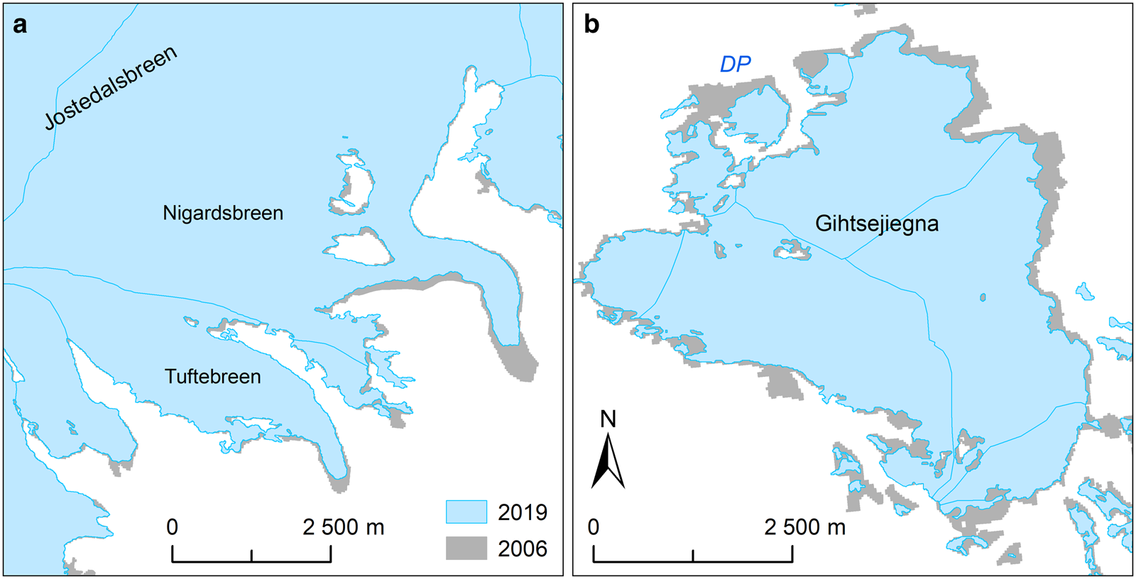
Fig. 13. Glacier changes comparing 2018–19 with 1999–2006 for (a) Nigardsbreen and Tuftebreen, outlets of Jostedalsbreen, (b) Gihtsejiegna. DP, detached parts from main glacier since 1999–2006. The individual mapping years are given. Note that map scale differs. The grey colour shows where the glaciers have shrunk from the previous to the current inventory. See Figure 1 for location.
Table 4. List of the ten largest glacier complexes in Norway and their change since the 1999–2006 inventory
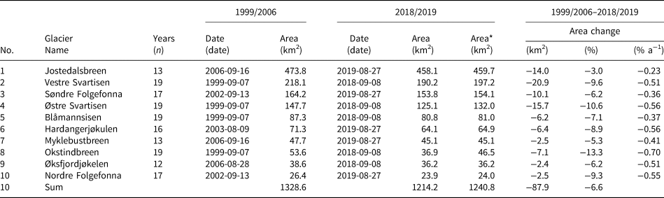
Area is the area of the complex, and area* includes parts disconnected in 2018–19 that were included in the 1999–2006 outlines. Glacier changes are calculated from the area of 1999–2006 and the area* of 2018–19.
Looking at the change of individual glaciers for the 3143 glaciers mapped in 1999–2006 reveal that most glaciers have shrunk between 1999–2006 and 2018–19. As expected, there is more variability for the smallest glaciers (Fig. 14). When inspecting the glaciers and comparing them with the 1999–2006 outlines, it was clear that in many cases, the smallest glaciers were mapped differently due to the higher resolution of Sentinel-2 (10 m) than Landsat (30 m). Moreover, the changes in ice divides and topology for some of the units give changes that are due more to methodology than actual glacier changes. Paul and others (Reference Paul2020) decided not to compare glacier by glacier from their 2003 Landsat inventory to their 2015 Sentinel-2 inventory for the European Alps as glacier-specific comparison was difficult due to differences in interpretation and a different location of the ice divides. Results must be interpreted with care for individual glaciers as the ruleset for glacier identification changes with different resolution of the datasets. We recommend checking orthophotos and the satellite imagery, as well as the glacier outlines from both inventories.
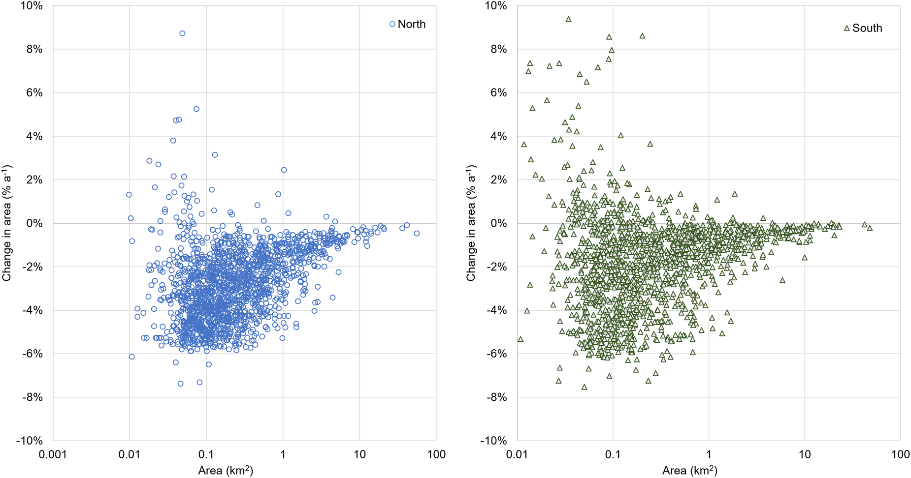
Fig. 14. Glacier change in % a−1 from 1999–2006 to 2018–19 for the 3143 glaciers mapped in 1999–2006 divided into (a) North and (b) South. Note that area scale is logarithmic. Area size is the original size in 1999–2006.
5.3. Glacier lakes
In total, we mapped 455 ice-marginal lakes in direct contact with the glaciers at the time of mapping. The surface areas of the lakes range in size from 0.00042 to 38.5 km2 (Storglomvatnet, Svartisen) with a total of 90.6 km2 and mean (median) of 0.20 km2 (0.15 km2). Of the lakes, 360 lakes with a total area of 10.1 km2 were newly formed or not mapped in the glacier lake inventory from 1999 to 2006 (Andreassen and Winsvold, Reference Andreassen and Winsvold2013). We mapped nearly 200 lakes that were not included in the 2018 product, mainly due to inclusion of lakes associated with glaciers in the size category 0.05–0.25 km2 that were not included in the 2018 mapping (Nagy and Andreassen, Reference Nagy and Andreassen2019; Andreassen and others, Reference Andreassen2021).
In our study, large lakes that have a clear glacier-ice interface were easy to identify and distinguish from the glaciers, whereas smaller and shallow lakes were more difficult to identify. Comparison with glacier lake and glacier outlines from 1999 to 2006 revealed a clear growth of many glacier lakes, formation of new lakes and some lakes no longer in contact with the glaciers (Fig. 15). For some glaciers, existing lakes have grown as glaciers have retreated such as Glacier ID 2532, a detached glacier that was connected to Spørteggbreen in the 1960s (Fig. 15a). Here images from 2006, 2014 and 2019 clearly show the retreat of the glaciers. While the two largest lakes were already present in 2006, new lakes have formed along the perimeter as the glacier has retreated (Fig. 15a). At the ice cap Hardangerjøkulen, many lakes have formed along the relatively flat western part that has been exposed as the ice has retreated (Fig. 15b). Vetlefjordsbreen from Jostefonni was calving in the lake in 2006 and the lake has continued to grow since then. The glacier has now retreated upslope and is no longer connected to the lake (Fig. 15c). Austerdalsisen from Østre Svartisen was also connected to the lake in the last inventory dating back to 1999 and has in recent years retreated from the lake. The distance to the lake was 150–200 m in 2018 (Fig. 15d). The glacier lakes of Vetlefjordbreen and Austerdalsisen were therefore not included in the 2018–19 dataset but are found in the historical glacier lake outline datasets. It was also clear that glacier lakes grew from 2018 to 2019 in southern Norway, by comparing the 2018 product with the updated product. Thus, Sentinel-2 can be used to show glacier lake growth at an annual scale. Some of the glacier lakes are dammed by the glacier or by moraines and are occasionally partly or fully drained. One of the glacier-dammed lakes, Demmevatnet at Rembesdalskåka, drained prior to 27 August 2019, the time of the mapping of Hardangerjøkulen. Here we included the lake perimeter from 4 August 2019 (Fig. S3).
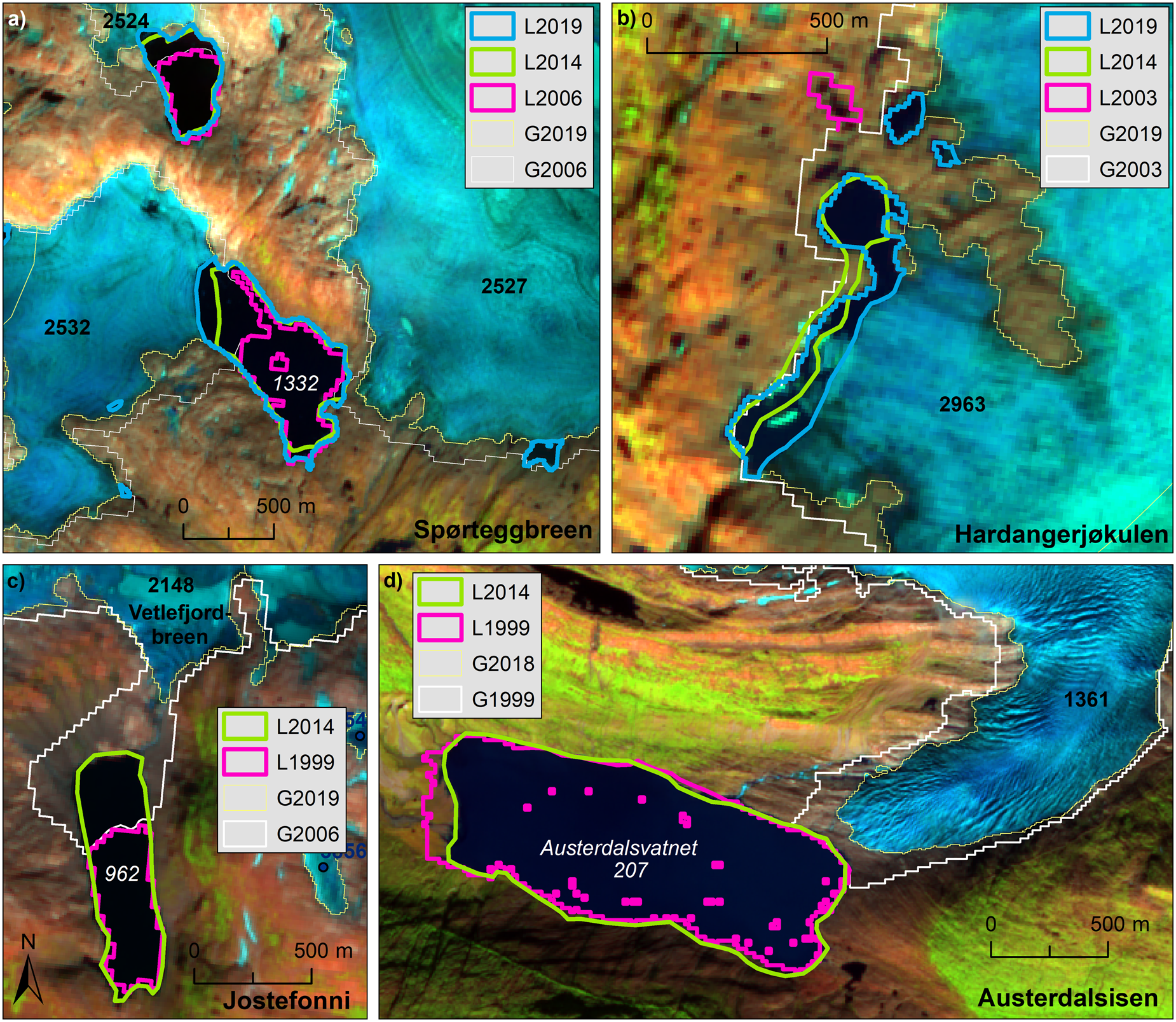
Fig. 15. Subsets of Sentinel-2 scenes (false 11-8-4) (a), (b) and (c) are scenes from 27 August 2019, (d) is a scene from 8 September 2018 showing glacier retreat, lake formation and growth between the previous 1999–2006 inventory and the current 2018–19 inventory. Lakes derived from Landsat images of 2014 are also shown. G, glacier outline; L, glacier lake outline and year denotes year of Sentinel-2 or Landsat image. (a) Part of Spørteggbreen (2527 and 2524) and detached patch 2532. (b)Part of western Hardangerjøkulen (2963) north of Rembesdalskåka. (c) Vetlefjordbreen (2148), part of Jostefonni where the glacier lake has grown, and the glacier has retreated out of the lake. (d) Austerdalsisen, outlet of Østre Svartisen, where the glacier was connected to the lake but now retreated upslope and is no longer attached. Elevations of lakes in white italic from norgeskart.no. Glacier IDs in black. /Copernicus Sentinel data/.
6. Discussion
6.1. On what to include in a glacier inventory
It can be challenging to decide what to include and exclude in an inventory. We wanted to include the parts containing ice, not seasonal or pure snowfields. In Norway, snowfields can be persistent and checking the available orthophotos revealed that many of them are long lasting and likely change little over time. For example, orthophotos and Landsat images from 2006 revealed minimal snow conditions in the Jostedalsbreen and Møre regions compared to more recent orthophotos and satellite images of 2019. Several years with mass surplus in the last decade (Andreassen and others, Reference Andreassen, Elvehøy, Kjøllmoen and Belart2020b) have resulted in transient growth of snowfields as well as glaciers. Snow conditions do not only depend on the current year but also on perennial snowfields that survive several years.
We mapped more smaller ice bodies than in the 1999–2006 inventory. An increase in the number of glaciers was also the case for the 1999–2006 inventory compared to previous inventories based on analogue aerial photography, with the explanation that automatic mapping typically includes more glaciers than manual digitising (Andreassen and others, Reference Andreassen, Winsvold, Paul and Hausberg2012). For example, in central Troms and Finnmark county, Leigh and others (Reference Leigh2019) found more glaciers using a semi-automated approach with cross-checking on 0.25 m aerial imagery, including 78 newly identified and mapped ice bodies in their analysis of the glacier area. Similarly, in the latest glacier inventory of the European Alps using Sentinel-2, Paul and others (Reference Paul2020) noted that many very small glaciers that are now included were not mapped or were mapped too small in the prior Alps-wide inventory (Paul and others, Reference Paul, Frey and Le Bris2011). The 2020 European Alps glacier inventory included 4395 units larger than 0.01 km2 (Paul and others, Reference Paul2020), while the 2011 inventory included 3770 units larger than 0.01 km2 (Paul and others, Reference Paul, Frey and Le Bris2011).
Sentinel-2 images can be used to observe ice and crevasses for larger glaciers, but this is more difficult on smaller bodies. A subregion of 161 km2 in Møre (Fig. 1) was chosen to compare differences between the classification we used for 2018–19 and the classification according to Leigh and others (Reference Leigh2019). Author 1 had controlled the automatically mapped polygons using Sentinel-2 imagery and orthophotos for the final 2018–19 outlines, while author 2 scored the polygons independently according to Table S3 using the orthophotos (Fig. 16). Results showed that for the 58 polygons, nine of them were classified as snow by author 2, representing an area of 0.101 km2. On the other hand, author 2 scored 20 of the classified snow polygons as ice patches and PSFs amounting to 0.004 and 0.062 km2, respectively, in total 0.066 km2. Moreover, author 2 also suggested to score many of the smaller ice patches as possible glaciers based on orthophotos, where there appeared to be an indication of crevassing and/or deformation of debris banding. Deformed debris bands may be remnants of former glacier flow, with the present-day ice body having shrunk to the point at which it retains their presence without any glacier motion.
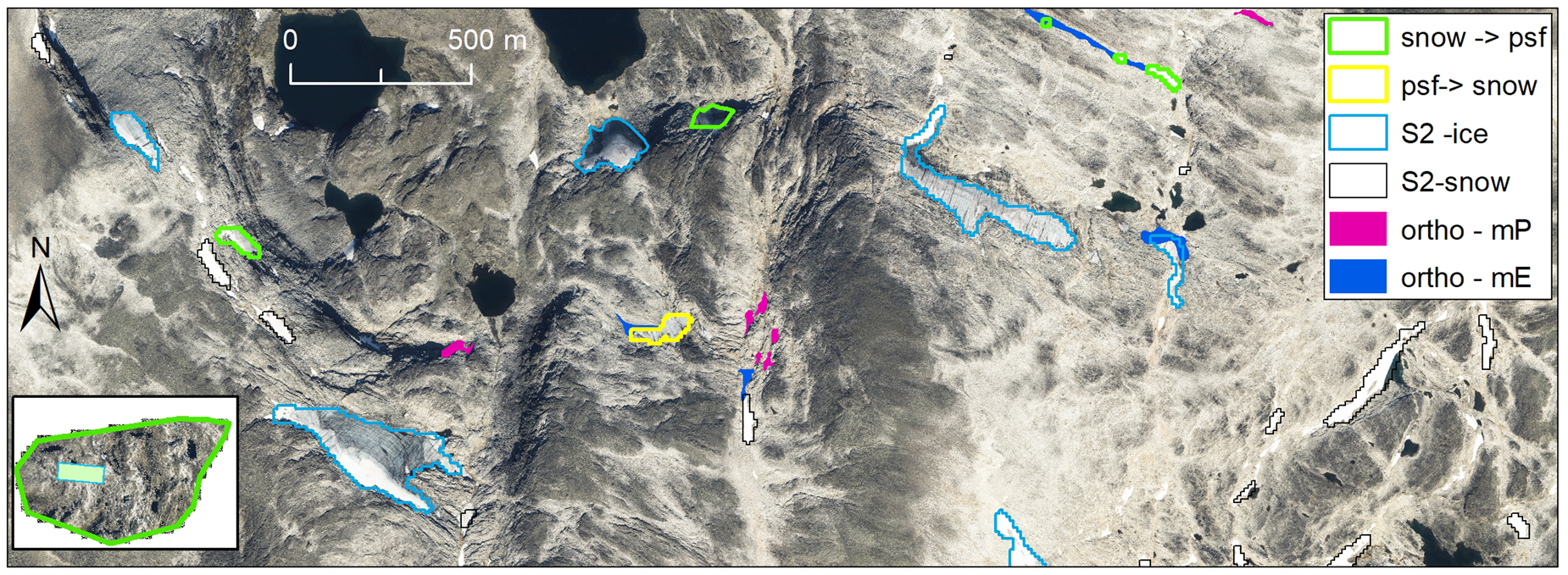
Fig. 16. Illustration of part of an area in Møre where the scoring system was tested on an orthophoto to classify glaciers, ice and snow using Sentinel-2. The inset shows the total area used for testing the scoring system and the extent of the part shown in detail. See Figure 1 for location. The green and yellow outlines reveal differences between the classification; green shows where snow was interpreted as ‘possible’ glaciers/ice patches and yellow where a classified ice patch was interpreted as snow using the scoring system. The filled polygons show where orthophoto scoring and mapping suggested inclusion of more possible glaciers/ice patches (ortho – mP) and more edits of the existing polygons (ortho – mE) in the 2018–19 inventory. Background orthophoto of 27 August 2019 from ©norgeibilder.no.
Furthermore, there is potential for very small glaciers (e.g.smaller than 0.5 km2) to persist in isolated topographic niches, with a high proportion of debris cover and/or extensive intense shading (e.g. Capt and others, Reference Capt, Bosson, Fischer, Micheletti and Lambiel2016; De Marco and others, Reference De Marco2020). These glaciers gain mass from wind-blown and avalanche snow (Helfricht and others, Reference Helfricht, Lehning, Sailer and Kuhn2015), gain mass and insulation from rock wall debris input (Bosson and Lambiel, Reference Bosson and Lambiel2016), are protected from solar radiation by relief (Olson and Rupper, Reference Olson and Rupper2019) and can be strongly influenced by permafrost conditions (Etzelmüller and Hagen, Reference Etzelmüller, Hagen, Harris and Murton2005). Very small glaciers can form at the base of rock walls, within recesses on steep valley sides, and/or impounded by large moraines or rock lips. Such glaciers are more likely to be missed or discarded in regional glacier inventories, especially those that rely on an automated component that is known to be more susceptible to miss shaded/debris-covered ice or which excludes potential false positives based on slope profiles. However, we are confident that we did not miss many ice bodies >0.1 km2 with the thorough inspection we did for this inventory.
Recently, Leigh and others (Reference Leigh2019, Reference Leigh, Stokes, Evans, Carr and Andreassen2020) identified several undocumented snow/ice-bodies in northern Norway that exist in heavily shaded niches, some of which are also debris covered. For example, Figure 17 shows two units that have not been recorded in any prior inventory or map: a ~0.02 km2 unit situated within a niche on a rock wall, ~140 m above glacier 123 (Figs17a–e) and a ~0.03 km2 partially debris-covered unit in an alcove below a rock wall and impounded by a large moraine (Figs 17f–i). On the Sentinel-2 imagery, it is difficult to discern the units or differentiate them from a snow patch (Figs 17e, i), and even on the aerial imagery from 2016 (Figs 17d, h), persistent snow cover prevents any identification of glacier ice. It has only been possible to determine the likely nature/origin of these units by viewing them in the field where oblique observations at a time with minimal snow cover (September) allow for ice, with debris banding to be detected (Figs 17b, g). It is not possible to obtain ground photographs for all ice/snow bodies across Norway. Therefore, it is highly likely that current limitations will inevitably mean some potential glaciers will be misclassified or remain undocumented.
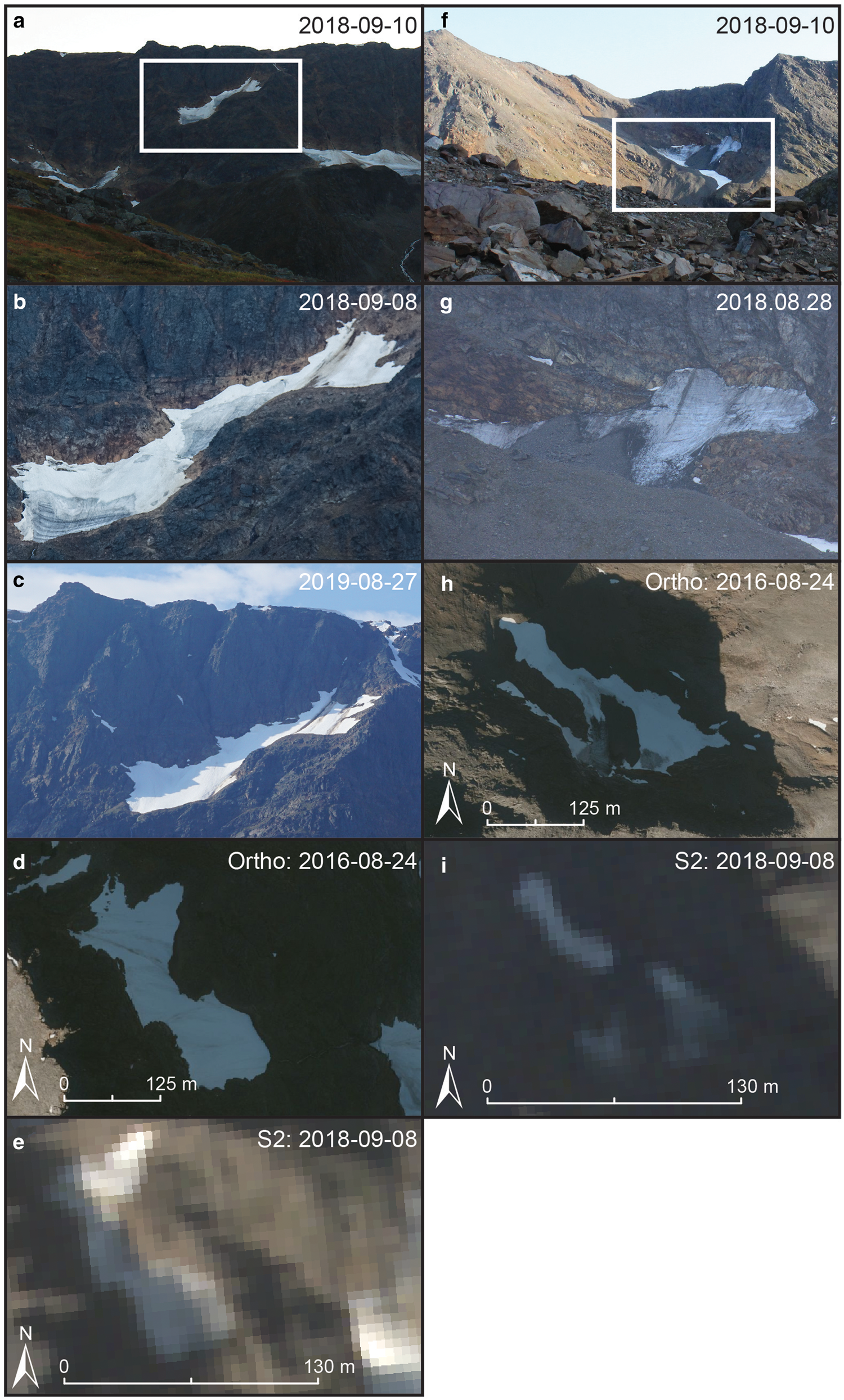
Fig. 17. Two very small ice bodies in the Kåfjord Alps (Troms and Finnmark county) first identified on high-resolution aerial imagery and subsequently viewed in the field. (a–e) A small (choose to refer to this as either ice/snow unit or glacier) within a niche on a rock wall above glacier 123; (a) oblique field photograph showing the ice/snow unit within the white rectangle, (b) zoomed in photograph showing bare ice, debris banding and a small ridge at its front, (c) a year later but with complete snow cover, (d) the unit from aerial imagery, (e) the unit from Sentinel-2 imagery. (f–i) A small glacier in an alcove below a steep rock wall, impounded by a large moraine, and partially debris covered; (f) oblique field photograph showing the ice/snow unit within the white rectangle, (g) a zoomed in photograph showing bare ice, some debris banding and debris cover, (h) the unit from aerial imagery, (i) the unit from Sentinel-2 imagery. /Copernicus Sentinel data 2018/© norgeibilder.no/.
6.2. Uncertainties in identifying and mapping very small glaciers on different image sources
In the central regions of Troms and Finnmark county (formerly classified as northern Troms and western Finnmark), Leigh and others (Reference Leigh, Stokes, Evans, Carr and Andreassen2020) used a semi-automated mapping approach on Landsat imagery from 2018 to map the glaciers and assess glacier changes. This is the same year as we used for our Sentinel-2 mapping in this region. In total, they mapped 252 glaciers on pansharpened Landsat-8 OLI imagery (15 m resolution; image date 28 July 2018) with a total glacierised area of 66.4 km2. Of the 252 glacier units mapped by Leigh and others (Reference Leigh, Stokes, Evans, Carr and Andreassen2020), 202 of these (equating to 65.29 km2) align with units mapped in this study using Sentinel-2 imagery (10 m resolution; equating to 61.52 km2), while the remaining 50 units (equating to 1.13 km2) were not included in the Sentinel-2 imagery. Furthermore, mapping conducted with the Sentinel-2 imagery identified an additional 139 units (equating to 1.38 km2) not mapped using Landsat-8 imagery. The differences in which glaciers were mapped in our inventory compared to Leigh and others (Reference Leigh2019) highlight the difficulty of identifying and mapping very small glaciers (<0.02 km2) from different image sources and using slightly different techniques.
Differences between our Sentinel-2 based glacier outlines and the aligned glacier units from the Landsat-8 based outlines can result in both larger and smaller units. For example, glacier ID 60 was mapped as 0.06 km2 on the Sentinel-2 imagery compared to 0.11 km2 on the Landsat-8 imagery (~0.05 km2 or 83% larger in area), whereas glacier ID 128 was mapped as 0.49 km2 on the Sentinel-2 imagery compared to 0.38 km2 on the Landsat-8 imagery (a ~0.12 or 29% smaller area: Fig. 18). On average, however, the Sentinel-2 derived outlines are ~0.02 km2 smaller than those mapped from Landsat-8 imagery, giving a smaller total area of the overlapping glaciers of 3.77 km2 (6%). The differences between the Sentinel-2 and Landsat-8 derived outlines for glaciers in valleys or cirques were smallest, even when considering the associated difficulties in mapping these units (e.g. heavy shading, supraglacial debris). The greatest differences were found for the glaciers located on elevated plateaus, such as glacier ID 120, which when mapped using Sentinel-2 imagery was definable as three separate units equating to a total area of ~0.08 km2. When mapped using Landsat-8 imagery it was depicted as one unit with an area of ~0.2 km2, representing an approximate 150% (0.12 km2) increase in the mapped glacier area. Mapping glaciers accurately is difficult at higher elevations, particularly owing to the prevalence of late-lying snow that can mask glacier boundaries.
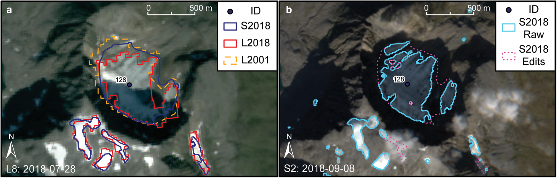
Fig. 18. Edited 2018 Sentinel-2 outlines (S2018), original 2018 Landsat 8 outlines (L2018; Leigh and others, Reference Leigh, Stokes, Evans, Carr and Andreassen2020), and original 2001 Landsat 7 outlines (L2001; Andreassen and others, Reference Andreassen, Winsvold, Paul and Hausberg2012); (b) unedited glacier outlines (S2018 Raw) and manual edits (S2018 Edits). Note: in (a) and (b) Landsat 8 (L8) and Sentinel-2 (S2) imagery are both shown in natural colours. /Copernicus Sentinel data 2018/.
There were also some differences associated with unit classification, whereby individual glacier/ice units are assigned specific classification (see Section 4.2, Table S3) based upon visual inspection of key glacial indicators (Leigh and others, Reference Leigh2019). The greatest differences in unit classification were found on those units smaller than 0.1 km2. Figure S7 provides an example of a previously unmapped body that has subsequently been mapped on Sentinel-2 imagery with an area of 0.03 km2 (this study) and on Landsat-8 imagery with an area of 0.05 km2 (Leigh and others, Reference Leigh, Stokes, Evans, Carr and Andreassen2020). Following the glacier scoring system, Leigh and others (Reference Leigh, Stokes, Evans, Carr and Andreassen2020) classified this new unit as a certain glacier based on the presence of multiple visual clues in the 2006 imagery (e.g.deformation of debris banding, evidence of multiple debris bands, bare ice, moraines in the recently deglaciated foreland). However, for the purpose of this study it was only classified as an ice patch/PSF. When such units are cross-checked on high-resolution colour orthophotos, interpretation and distinction between glacier ice vs remnant glacier ice vs non-glacial ice patches remains challenging, especially when there are unfavourable snow conditions (e.g. Figs S7d, e).
While there are undoubtedly differences in associated glacier area resulting from varying image resolution, differences also result from image capture date and time as extent and intensity of shading will change throughout the year and day. The mapping date of the Landsat-8 imagery was earlier in the melt season (28 July 2018) than the Sentinel-2 imagery (8 September 2018). The prevalence of late-lying snow has the potential to mask glacier boundaries, making the unit appear larger than it really is (Fig. 18). The smaller total area (6%) in the overlapping area in our Sentinel-2 mapping compared to the Landsat-8 mapping illustrates how results can differ within the same year. The end of July is probably a bit too early for optimal glacier mapping and it is in general better to use images from later in the season. We mainly used dates from the 1 or 8 September 2018 for northern Norway and 27 August 2019 for southern Norway for our 2018–19 inventory. Earlier scenes from 4 and 15 August 2019 had to be used for some glaciers in southern Norway due to clouds (Fig. 2). Thus, a compromise of image capture date may be needed to secure imagery from the necessary year, at the risk of overestimating the glacier area. Substantial cloud cover over the coastal areas of Norway results in a decreased availability of appropriate satellite imagery (e.g. Winsvold and others, Reference Winsvold, Andreassen and Kienholz2014). While Sentinel-2 provides a better temporal resolution (5-day repeat cycle, more frequent at the higher altitudes), Landsat-8 (16-day repeat cycle) is still valuable for glacier change detection.
Comparing the four largest glacier composites in the overlapping Landsat-8 and Sentinel-2 sample for Troms and Finnmark county shows that all glaciers are larger in Landsat-8 mapping than in the Sentinel-2 mapping (Fig. S4). The four ice caps had a total area of 49.9 km2 in Landsat-8 and 48.3 km2 in Sentinel-2, thus the glacier area was 3.3% larger from Landsat-8. The area derived from outlines digitised from Pléiades imagery for two of the glaciers, Langfjordjøkelen and Øksfjordjøkelen, as described in Section 4.5.5 was smaller (Table 5, Fig. 12, Fig. S4). Compared to Sentinel-2 (36.3 km2), the Pléiades area was −1.2% smaller (35.9 km2) and the Landsat area was 2.5% larger (37.3 km2). Again, the Landsat-8 mapping was conducted on an earlier image and a true comparison would need a closer time gap between acquisition dates. The agreement in mapped area between the Pléiades orthoimage and Sentinel-2 imagery shows that Sentinel-2 can be used for accurate glacier mapping for clean ice with limited shadowing.
Table 5. Comparison between glacier outlines of the largest four glaciers in the central region of the Troms and Finnmark county using three different imagery types with different image capture dates in 2018: Sentinel-2 (S2) (10 m) of 8 September, pansharpened Landsat-8 (L8) (15 m resolution) of 28 July, and Pléiades (P) (0.5–2 m resolution)
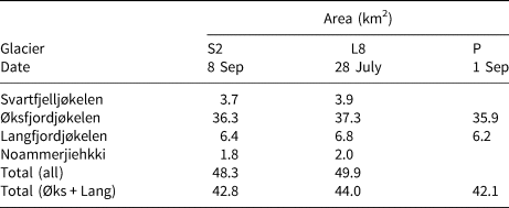
Note that for the Sentinel-2 imagery-based outlines for Landfjordjøkelen, the Pléiades image and outlines were compared when deciding the ratio and as such, these outlines are not independent. See Figure 12 for the Pléiades imagery of Øksfjordjøkelen.
6.3. Uncertainty estimates and validation
In the 1999–2006 inventory, an overall uncertainty of 3% was estimated, using validation data in a subset of glaciers in one region. The uncertainties in estimating the area of glaciers and glacier lakes from the new 2018–19 inventories have been assessed in this study using orthophotos and Pléiades orthoimages and testing out band ratio and band 2 thresholds. This revealed that the relative uncertainty increased with decreasing glacier size. An overall uncertainty between <1 and 3% can be expected, but individual uncertainties can be much larger for the smallest glaciers. Although we had good validation datasets from Pléiades and orthophotos, these were also partly challenging to analyse due to dark ice in some parts (Figs 7, 8). To assess the real accuracy, we need to compare our estimates with field measurements. Even with validation data as we have there, we do not have ground truthing. Our manual digitisation revealed that both the number and area of mapped glaciers varied between the digitisers. Still, results showed good overall agreement and revealed that the Sentinel-2 band ratio-based mapping worked well, except for parts in shadow or with debris where the uncertainties are larger. We conclude that for clean ice, the Sentinel-2 semi-automated mapping has an accuracy comparable to manual digitising from high-resolution data.
Another common method is to assess the uncertainty using the buffer method, by applying a negative or positive buffer around glacier outlines. This also reflects the sensitivity of the result. We assessed this impact by applying a negative or positive buffer around glacier outlines. Assuming an uncertainty along the perimeter corresponding to the Sentinel-2 10 m pixel size, we created buffers of ±5 and ±10 m around the glacier and glacier lake polygons. For all the glacier polygons, a ±5 m buffer resulted in a change in area of ±3.1%, increasing (decreasing) the glacier area to 2401 (2257) km2 (Table 6). A ±10 m buffer nearly doubles the area change to ±6%. Looking at Jostedalsbreen, the largest glacier complex, the impact of a ±5 and ±10 m buffer was an area change of ±1.1 and ±2.3%, respectively. For the ten largest glaciers, the impact of a ±5 and ±10 m buffer was an area change of 1.0 and ±1.9%, respectively. For rounder glaciers, the impact will be smaller; for elongated glaciers, the impact will be larger. The smallest glaciers have the largest relative changes in area, e.g. for a small ice patch like Juvfonne (0.1 km2), the impact of a ±5 and ±10 m buffer was ±9 and ±18%, respectively. The Juvfonne area was derived from Sentinel-2 on 4 August 2019 (not 27 August due to clouds) and is 0.106 km2, whereas the outlines derived from the orthophoto from 26 August 2019 give an area of 0.087 km2 (Fig. 19). This was indeed the same as an 18% reduction, but part of the difference is due to melting around the perimeter in the 22 days from the Sentinel-2 acquisition compared to the orthophoto acquisition. Snowy parts in the southwestern part were included in the Sentinel-2 automatic outline, but not in the manual digitisation from the orthophoto due to melting (Fig. 19). For this thin ice patch, the variations around the perimeter are large from year to year and during the melt season (Ødegård and others, Reference Ødegård2017; Andreassen and others, Reference Andreassen, Callanan, Saloranta, Kjøllmoen and Nagy2020a).
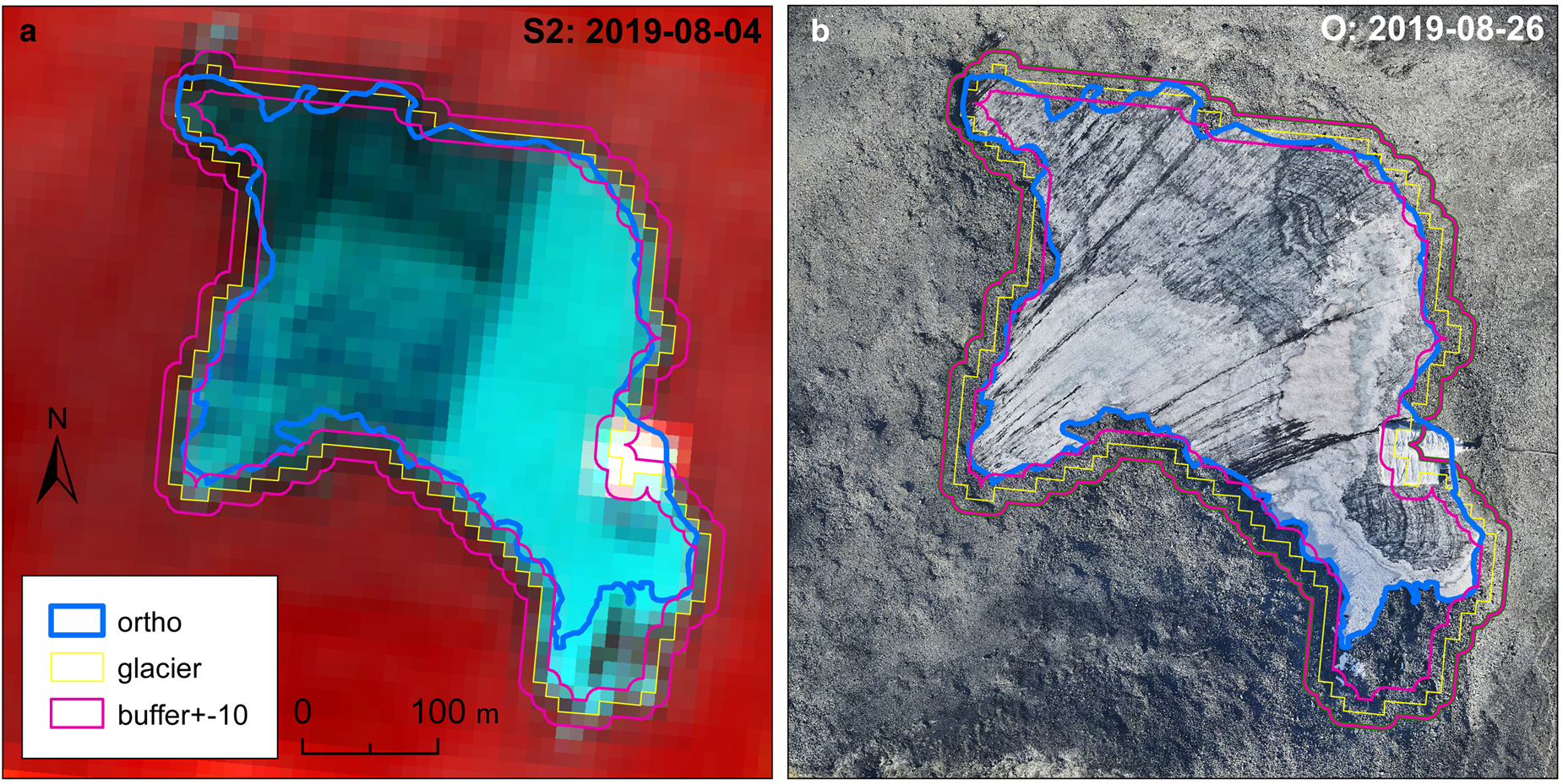
Fig. 19. Effect of a ±10 m buffer around the glacier polygons on the total area extent of Juvfonne with (a) Sentinel-2 image of 4 August 2019 in the background and (b) orthophoto of 26 August 2019 in the background. Ortho, outline manually digitised from orthophoto; glacier, automatically mapped from Sentinel-2. See Table 6. /Copernicus Sentinel data 2019/orthophoto Terratec/NVE/.
Table 6. Sensitivity of buffer of size ±5 and ±10 m around the glacier polygons on the total area in % for all of Norway and a selection of the ten largest and some different sizes
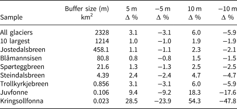
Δ – Difference. See Figure 1 for location of glaciers.
In this study, we validated our S2-mapping to manual digitisations from orthophotos and orthoimages, tested the sensitivity of different thresholds and tested the sensitivity by applying buffers. A summary of these tests shows that for glaciers larger than 0.3 km2, relative area differences are within 7% (Table 7). The validation data reveal larger relative differences for smaller glaciers, similar to what we see for the buffer method (Table 6). The result for the smallest glaciers was very sensitive to manual edits and snow conditions at the time of mapping. The S2-areas were both smaller and larger than the area derived from the validation data. For groups of glaciers, the relative area differences were smaller. Based on our validation results, we find them in a line with a ±5 m buffer for all of Norway. Thus, we estimate the total uncertainty in the glacier area of Norway to be ±3% or 70 km2. The reduction in glacier area from 1999–2006 to 2018–19 ranges between 364 and 411 km2 or 14 and 15%, depending on whether we compared the total area from 2018 to 2019 with the total area from 1999 to 2006 (13.5%), the total area from 2018 to 2019 with 1999–2006 including the PSF (14.3%), or only glaciers mapped both in 2018–19 and 1999–2006 (15.3%). The reduction in area was for all samples larger than the uncertainty in the total areas of both 1999–2006 (3%, 81 km2) and 2018–19 (3%, 70 km2).
Table 7. Summary of validation and sensitivity tests and other comparisons in this study
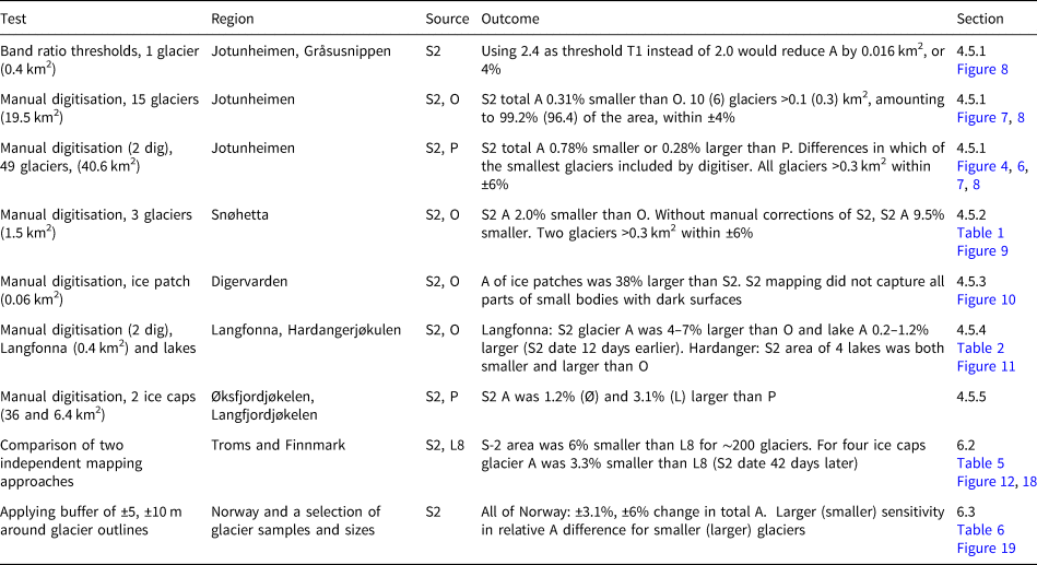
A, area; S2, Sentinel-2; L8, Landsat-8; O, aerial orthophoto; P, Pleiades satellite orthoimage. All S2 areas refer to the final edited result unless noted. One digitisation per object unless noted (2 dig) in first column. See Figure 1 for location of the glaciers.
The accuracy of the glacier lake mapping was tested for a sample of five lakes and revealed relative differences within ±1.5% for two of the lakes >0.1 km2. For a lake that had floating ice and the two smallest lakes, a relative difference of up to 16% was found. The accuracy of the semi-automated glacier lake mapping using NDWI for the 2018 lake outlines was also tested using manual digitisations of nine lakes from orthophotos from norgeibilder.no and revealed a 4% accuracy (Nagy and Andreassen, Reference Nagy and Andreassen2019). The impact of different image acquisition dates on lake area was also assessed for a subset of seven lakes around Hardangerjøkulen over the period 13 July–3 September 2018, where snow cover and terrain-induced shadowing varied. The differences between the smallest and largest area of each lake ranged from 1.5 to 6.2% (Nagy and Andreassen, Reference Nagy and Andreassen2019). From our findings, we estimate an accuracy of the glacier lake mapping within 3% for glacier lakes >0.1 km2, except for glacier-lake interfaces with floating ice.
7. Conclusions
In this study, we used Sentinel-2 images from 2018 (northern Norway) and 2019 (southern Norway) to produce an updated dataset of glacier and ice-marginal lake outlines. We validated our glacier outline and glacier lake mapping with aerial orthophotos (0.25 m resolution) and Pléiades satellite orthoimages (0.5–2 m resolution) and tested the sensitivity by creating buffers around the glacier perimeter (Table 7). Overall, we estimated the accuracy within 3% for the overall glacier and glacier lake datasets. For the smallest ice or lake bodies, relative uncertainties were larger. A total of 60% (1400 km2) of the glacier area is in southern Norway and 40% (928 km2) is in northern Norway. The total glacier area is now 2328 ± 70 km2, a reduction in glacier area by 15% when comparing only the glaciers mapped in the previous inventory 1999–2006. The 10 largest glacier complexes accounted for 1214 km2 (52%) of the total area and have been reduced by 6.6% since 1999–2006. The area reduction has been largest in northern Norway (22%), compared to southern Norway (10%), but it should be noted that the period between inventories was larger for northern Norway. The 36 glacier regions have decreased in area ranging from −3 to −0.03% a−1. In Norway, the regions with the largest percentage changes were dominated by small glaciers, and the regions with smallest percentage changes were dominated by the largest glaciers.
In total, over 2000 small glaciers and ice patches totalling 37 km2 were mapped in this new 2018–19 dataset that were not included in the previous 1999–2006 glacier inventory. This was in part due to the higher resolution of Sentinel-2 (10 m) than Landsat (30 m), which was used for the previous inventory. All glacier bodies were carefully inspected using Sentinel-2 images, orthophotos and topographic maps. It is, however, noted that some smaller units (<0.1 km2) and parts of glaciers may still have been missed or excluded due to snow conditions, clouds, cast shadow, debris cover or misinterpretations. Some large bodies (>0.1 km2) classified as snow and not included in the 2018–19 inventory may have ice content. We applied manual edits to correct for glacier lake interfaces, debris cover, heavy shading and sometimes to detach snow patches. The manual editing needed to detach glacier lakes was used to produce an updated glacier lake outline dataset for 2018–2019 to match the new 2018–19 glacier outlines. We mapped 455 ice-marginal lakes that appeared to be in direct contact with the glaciers at the time of mapping, whereof 360 were new since the lake inventory from 1999 to 2006.
Our work demonstrated that it was easier to find scenes from Sentinel-2 than from Landsat used in the previous inventories due to the higher temporal resolution of Sentinel-2. We were able to cover all of mainland Norway over two subsequent years, 2018–2019, whereas the previous 1999–2006 inventory used scenes from a 7-year period. Using Sentinel-2 or Landsat-8 images from earlier in the melt season led to an overestimation of the glacier area due to more seasonal snow. However, early scenes were useful to check parts in shadow due to less terrain-induced shadowing. The higher spatial resolution of Sentinel-2 made it easier to identify smaller glaciers and lakes than in the previous glacier and glacier lake inventories. Orthophotos are a good supplement for training, validation and classification and can be used to create inventories in smaller regions. Deriving glacier and glacier lake outlines from orthophotos for all of mainland Norway over a short time interval is not yet possible with the data available at norgeibilder.no. The orthophotos span a too long period and many of them have adverse snow conditions. Using Sentinel-2 images and applying the standard semi-automated method with band ratio and manually selecting thresholds mapped clean ice accurately. Careful inspection of all bodies and manual corrections were however needed. Manual inspection is time consuming and prone to errors. Differences in human interpretation or difficult mapping conditions due to snow, debris or clouds still cause uncertainties and inhomogeneities in the result. For the glacier lake mapping, we used both NDWI calculations and manual digitisation. We found that the accuracy in the semi-automatic mapping used here is as accurate or better than automatic approaches using NDWI and can be faster for a region of the size of mainland Norway.
Supplementary material
The supplementary material for this article can be found at https://doi.org/10.1017/jog.2022.20.
Data
The previous glacier outlines and glacier lake outlines are available at https://nve.brage.unit.no/nve-xmlui/handle/11250/2830933 as part of the CryoClim collection. The new 2018–19 glacier outlines and lake outlines are available at: https://nve.brage.unit.no/nve-xmlui/handle/11250/2828121 as part of the Copernicus glacier service collection. The glacier and glacier lake outlines are submitted to GLIMS https://www.glims.org/. We there included a few glacier outlines on the border between Norway and Sweden. The Swedish parts of the glaciers are not included in the glacier area of Norway.
Acknowledgements
We thank editor Fanny Brun and associate chief editor Nicolas Cullen for handling the manuscript and reviewer Frank Paul and one anonymous reviewer for numerous comments that improved the manuscript. This work is a contribution to the project Copernicus bretjeneste (Copernicus Glacier Service Norway, Contract NIT.06.15.5/NIT.08.19.5) and to the JOSTICE, CryoClim and FonnSat projects. We thank Solveig H.Winsvold (NVE) for work on the Copernicus project and for making processing scripts available. We thank the European Space Agency for providing freely available Sentinel-2 imagery and for providing orthorectified imagery using the Norwegian DTM. We thank Etienne Berthier (LEGOS) and Centre National d'Etudes Spatiales (CNES) for providing Pléiades orthophotos. We thank Ivar Peerebom (NVE) for geodatabase design and updates of NVE's digital glacier atlas. Paul Weber digitised the Pléiades outline of Øksfjordjøkelen. Chris Stokes (Durham University), Rune Engeset (NVE) and Hallgeir Elvehøy (NVE) provided valuable comments to the manuscript. George Stanley Cowie provided language corrections and valuable comments.
Author contribution
T.N. selected, downloaded and processed the satellite images. L.M.A. and T.N. edited the glacier and glacier lake outlines and prepared the glacier and glacier lake 2018–19 datasets for southern and northern Norway, respectively. L.M.A. prepared the final datasets, created figures and tables, analysed results and wrote the text with contributions from T.N., B.K. and J.R.L. All authors digitised glacier outlines for validation and read and commented on the manuscript.


 Open access