


1. INTRODUCTION
Calving is one of the most important processes in the mass loss of glaciers; it is a major contributor to the observed and predicted sea-level (Benn and others, Reference Benn, Warren and Mottram2007b). Recent estimates show that it contributes ~50% of the mass loss of the Antarctic (Rignot and others, Reference Rignot, Jacobs, Mouginot and Scheuchl2013) and Greenland (van den Broeke and others, Reference van den Broeke2009) ice sheets and is expected to increase even more with climate warming. Despite rapid advances in modelling and field observations, there is still a large knowledge gap concerning the triggering of particular calving events. One of the reasons for this is a deficiency of detailed quantitative observations of such events, especially those of a smaller size. Most of the focus of the scientific community is on large outlet glaciers draining the Antarctic and Greenland ice sheets (e.g. Rignot and others, Reference Rignot, Mouginot, Morlighem, Seroussi and Scheuchl2014; Murray and others, Reference Murray2015; Ryan and others, Reference Ryan2015), whereas smaller glaciers have been studied less. One reason for this is their relatively low impact on global-scale issues, like sea-level rise. Nevertheless, in some areas these smaller glaciers with relatively low ice flow velocities are most common and hence their calving is of great importance for regional-scale issues as glacial retreat, regional mass balance or fresh water input into local ecosystems. The South Shetland Islands are a perfect example of such a region. Due to the exposure to one of the most striking examples of air temperature rise in recent years (Vaughan and others, Reference Vaughan2003; Turner and others, Reference Turner2005; Kejna and others, Reference Kejna, Araźny and Sobota2013) large ice mass losses are observed in the area of northern Antarctic Peninsula (Cook and others, Reference Cook, Fox, Vaughan and Ferrigno2005; Hock and others, Reference Hock, de Woul, Radić and Dyurgerov2009). Nonetheless, given the observed climate change, the frontal retreat of the South Shetland Island glaciers is, mostly because of their topography, relatively small compared with other regions of the world (Osmanoglu and others, Reference Osmanoglu, Braun, Hock and Navarro2013, Reference Osmanoglu, Navarro, Hock, Braun and Corcuera2014). The South Shetlands mostly comprise small ice caps with few outlet glaciers, where the bulk of the ice cliffs terminate in the ocean on a high-water level mark, in the intertidal zone (Hughes and Nakagawa, Reference Hughes and Nakagawa1989). This inhibits calving and limits oceanic influences, such as submarine melt or high-strain rates due to low basal pressure. Nevertheless, calving dominates ice mass loss of glaciers on the South Shetland Islands because of very low surface ablation rates (Navarro and others, Reference Navarro, Jonsell, Corcuera and Martin-Espanol2013; Osmanoglu and others, Reference Osmanoglu, Navarro, Hock, Braun and Corcuera2014).
Despite recent advances in calving measurements stimulated by the development of new high-resolution surveying methods, for example terrestrial laser scanning (TLS) (e.g. Schwalbe and others, Reference Schwalbe, Maas, Dietrich and Ewert2008; Pętlicki and others, Reference Pętlicki, Ciepły, Jania, Promińska and Kinnard2015), Structure-from-Motion photogrammetry (e.g. Ryan and others, Reference Ryan2015) or terrestrial radar interferometry (e.g. Rolstad and Norland, Reference Rolstad and Norland2009; Voytenko and others, Reference Voytenko2015), there is still a lack of detailed quantitative observations of single calving events (Chapuis and Tetzlaff, Reference Chapuis and Tetzlaff2014). Other techniques for example, visual observations (e.g. Chapuis and Tetzlaff, Reference Chapuis and Tetzlaff2014), indirect methods like underwater accoustics (e.g. Glowacki and others, Reference Glowacki2015) and seismic observations (e.g. O'Neel and others, Reference O'Neel, Larsen, Rupert and Hansen2010), lack sufficient precision to quantify ice volume loss during calving events. On the other hand, the classical remote sensing methods like repeat satellite imagery analysis or airborne photogrammetry have limited temporal resolution and therefore are best suited for tracking of particularly large calving events (e.g. Joughin and MacAyeal, Reference Joughin and MacAyeal2005). Moreover, they are often restricted to measuring aerial changes and thus need to be parameterized with other methods to yield volume estimates.
TLS is now widely recognized as a precise, rapid and extremely useful method of surveying snow cover (e.g. Prokop, Reference Prokop2008; Egli and others, Reference Egli, Jonas, Grünewald, Schirmer and Burlando2012; Deems and others, Reference Deems, Painter and Finnegan2013; Hartzell and others, Reference Hartzell, Gadomski, Glennie, Finnegan and Deems2015) and glacial dynamics (e.g. Schwalbe and others, Reference Schwalbe, Maas, Dietrich and Ewert2008; Pętlicki and others, Reference Pętlicki, Ciepły, Jania, Promińska and Kinnard2015). Despite the high cost of TLS relative to other techniques like Structure-from-Motion photogrammetry (Westoby and others, Reference Westoby, Brasington, Glasser, Hambrey and Reynolds2012), its high-spatial resolution and precision remains unparalleled (Passalacqua and others, Reference Passalacqua2015).
In recent years calving models have undergone a major change towards better description of the processes involved, from bulk models forced by an independent environmental variable like height-above-buoyancy (e.g. Vieli and others, Reference Vieli, Jania and Kolondra2002), through the crevasse depth criterion of Benn and others (Reference Benn, Hulton and Mottram2007a) implemented in several cases (Amundson and Truffer, Reference Amundson and Truffer2010; Nick and others, Reference Nick, van der Veen, Vieli and Benn2010; Otero and others, Reference Otero, Navarro, Martin, Cuadrado and Corcuera2010), to most recent models that account for damage mechanics (Krug and others, Reference Krug, Weiss, Gagliardini and Durand2014) and are able to reproduce the crevassing of the terminal part of tidewater glaciers as well as the time and size distribution of individual events (Åström and others, Reference Åström2013, Reference Åström2014). The most recent and sophisticated models require much more precise calving size distribution data to validation purposes, but such data are scarce (Åström and others, Reference Åström2014; Chapuis and Tetzlaff, Reference Chapuis and Tetzlaff2014). The main goal of this work is to provide a detailed catalogue of the size distribution of calving events on Fuerza Aérea Glacier together with a methodology that allows for precise quantitative monitoring of calving.
2. STUDY AREA
Greenwich Island is located in the South Shetland Islands, Antarctica, a global ‘hot-spot’ of climate change, where a significant warming has been observed since the 1950s with a positive air temperature trend of 0.3°C (10 a)−1 (Vaughan and others, Reference Vaughan2003). It is one of the 11 major islands of the archipelago with a surface area of 142 km2. Despite being located in the centre of the archipelago it has not drawn much attention from the physical sciences, except only a few glaciological, geomorphological or oceanographical studies (e.g. Arcos and Salamanca, Reference Arcos and Salamanca1980; Azhar and Santana, Reference Azhar and Santana2007; Santana and Dumont, Reference Santana and Dumont2007). Much more attention has been given to the neighbouring Livingston Island (e.g. Otero and others, Reference Otero, Navarro, Martin, Cuadrado and Corcuera2010; Navarro and others, Reference Navarro, Jonsell, Corcuera and Martin-Espanol2013; Osmanoglu and others, Reference Osmanoglu, Navarro, Hock, Braun and Corcuera2014) and particulary to the largest island of the archipelago, King George Island, where the surface mass balance (e.g. Knap and others, Reference Knap, Oerlemans and Cadée1996; Braun and Hock, Reference Braun and Hock2004; Sobota and others, Reference Sobota, Kejna and Araźny2015) and ice dynamics (e.g. Simoes and others, Reference Simoes, Bremer, Aquino and Ferron1999; Rückamp and others, Reference Rückamp, Blindow, Suckro, Braun and Humbert2010, Reference Rückamp, Braun, Suckro and Blindow2011; Osmanoglu and others, Reference Osmanoglu, Braun, Hock and Navarro2013; Sobota and others, Reference Sobota, Kejna and Araźny2015) have been investigated in detail. Although the Greenwich Island ice cap is part of the Antarctic periphery inventory (Bliss and others, Reference Bliss, Hock and Cogley2013), its actual calving flux remains unknown.
Fuerza Aérea Glacier (Fig. 1) is one of the outlet glaciers of the Greenwich Island ice cap. It is located in the eastern part of Greenwich Island, has a width of ~4.5 km, length of 2 km and area of 7.26 km2 (WGMS, 1989). The glacier flows from the northwest slopes of the Breznik Heights into the eastern coast of Discovery Bay. Fuerza Aérea Glacier is typical of outlet glaciers found on South Shetland Islands; it has relatively low calving rate, high crevassing in the terminal part due to a steep slope next to the front, and a terminus partly grounded at the high-water mark (with bedrock at the terminus submerged during high tides and exposed at low tides).
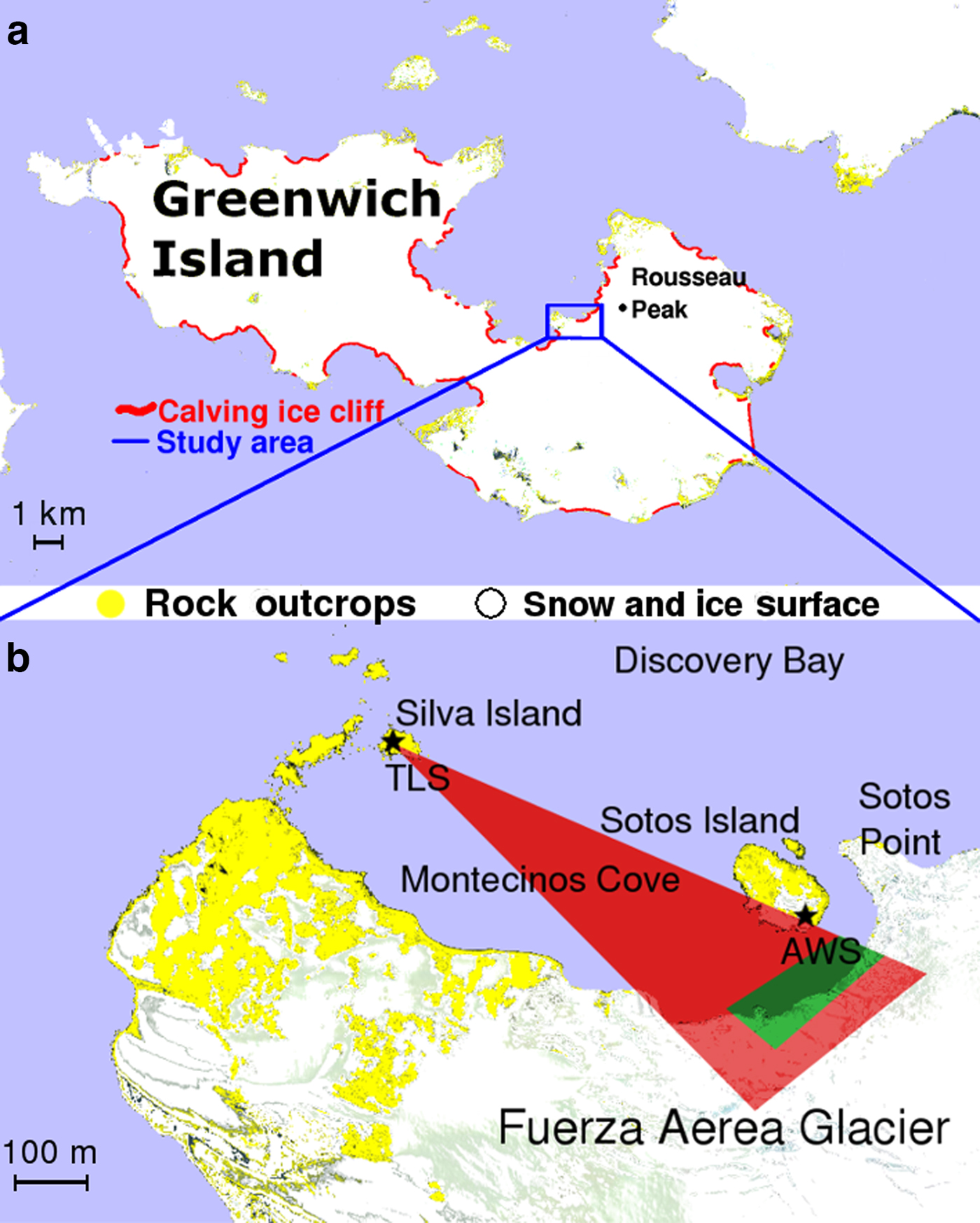
Fig. 1. Location of the study site: (a) Greenwich Island, (b) Surroundings of Fuerza Aérea Glacier showing the imposed scanned area (red), the investigated part of the ice cliff (green), TLS and AWS.
3. DATA AND METHODS
Results from TLS surveys and continuous video recording have been combined to assess volume changes of the active ice cliff of Fuerza Aérea Glacier. TLS was used to measure the volumes of individual calving events by differentiating subsequent point clouds, whereas the video provided continuous recordings of calving activity that were used to map the calved ice area. Because the front is grounded in very shallow water we assume the underwater calving on Fuerza Aérea Glacier is neglible. Therefore, the calved ice area is assumed to be equal to the area of the scar produced by calving on the subaerial part of the ice cliff. An empirical calved ice area/volume relationship was used to scale the areas derived by video observations to ice volumes using the TLS measurements as a reference. Finally, the record of calved ice volume was compared with potential environmental drivers of calving.
3.1. Video monitoring
A Mobotix MX-M24-M video camera with a 32 mm lens was installed on Sotos Island at the automatic weather station (AWS) site located 120 m from Fuerza Aérea Glacier (Fig. 1), overlooking the active ice cliff. Between 21 January and 04 February 2013 the camera continuously recorded a video of the ice cliff with a time resolution of 8 frames s−1 and image resolution of 800 × 600 pixels. Calving events were tracked by visual inspection of the video frames immediately before and after each calving event. Areas of calved ice were mapped manually with Quantum GIS software (Fig. 2) and the associated polygons were exported to a shapefile. Polygons areas were expressed in pixels in a local coordinate system. Next, they were georeferenced by projecting them onto TLS-derived point clouds of the ice cliff using easily discernible features, such as crevasses, as a reference.
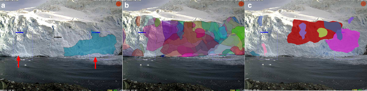
Fig. 2. Calving events of Fuerza Aérea Glacier identified on video recording. (a) An example from 21 January 2013. (b) Complete record for 21 January–04 February 2013. (c) Nine events that did not occur from the same space on the calving cliff as others during the time interval between TLS measurements. Areas of different color are areas of the cliff that failed, red arrows indicate fallen ice accumulated in shallow water.
3.2. Terrestrial laser scanning
Surveys were made with Optech ILRIS-LR terrestrial laser scanner, a state-of-the-art instrument dedicated to topographic measurements of snow and ice surfaces. It has a wavelength of 1064 nm and a nominal operating range of 3000 m; however, low reflection from clean ice limited range to 1000 m (Pętlicki and others, Reference Pętlicki, Ciepły, Jania, Promińska and Kinnard2015). The scanner was placed on Silva Island (Fig. 1) at a distance of ~800 m from the active ice cliff, which is in Montecinos Cove. The investigated part of the ice cliff is located south of Rousseau Peak next to Sotos Point and the neighbouring unnamed island, herein referred to as Sotos Island.
The sampling rate of the Optech ILRIS-LR is 30 kHz, hence 30 000 points s−1 are acquired. However, the instrument was running in the field only for short periods, when meteorological conditions were suitable (no fog, precipitation or strong winds that could affect the measurements) and the sea conditions allowed reaching Silva Island from Arturo Prat Station. Therefore, throughout the observation period of 14 d (21 January–04 February 2013) only 6 TLS measurements were taken on 21, 25, 31 January and 1, 2 and 4 February 2013. Water vapour decreases the operating range and the quality of the return signal of the laser scanner and hence measurements cannot be made in poor visibility.
The measurement itself normally took a few hours, as a larger portion of the Montecinos Cove, than only the investigated part of the ice cliff, was scanned (Fig. 1), in order to capture ice-free areas that could be used for the point cloud alignment into a common reference frame.
The raw data stored in the scanner constitute of points in polar coordinates (azimuth angle, elevation angle, range from the scanner centre), together with their associated intensity of reflection and shot flags. Thus, the file can be regarded as a raw point cloud in polar coordinate system. Pre-processing was performed in Optech ILRIS Parser software and involved (1) trimming the point cloud, (2) applying the atmospheric correction for range, (3) change of polar coordinate system to Cartesian and (4) exporting the resulting point cloud to PTX format, Leica exchange format. The atmospheric correction applied was linear in range and accounted for air humidity, pressure and temperature.
Next, the point clouds were imported into the Cloud Compare software and georeferenced using four ground control points located on stable bedrock (Silva and Sotos Islands, Ferrer Point) in the vicinity of the glacier. Point clouds were then aligned using exposed bedrock on the islands and next to the ice front. The associated 3-D error, calculated as a RMS deviation between the point clouds, varies between 7 and 19 cm.
The displacements between the point clouds were calculated along the flow direction. Ice advection displacements were low compared with the lengths of the calved ice blocks, thus an increase in distance from the scanner to the ice cliff was associated with calving, whereas a decrease was associated with ice front advance. Regions that did not experience calving in successive point clouds were used to calculate ice advection; ice velocities were assumed constant over the entire ice cliff apart from nine non-overlaying calving events that were used for area/volume scaling; for these local ice advection was calculated from their respective histograms of displacements. Ice advection was calculated from the maximum positive peak in the histograms of displacement along the width of the terminus. The length of calved ice blocks was obtained by adding the calculated local ice advection value to the increase in distance measured between the scanner and the ice cliff.
3.3. Area/volume scaling
The relation between area and volume is assumed to be a polynomial of degree 3/2, i.e. the length of the calved ice block is proportional to the square root of its area. In other words, the length x is linearly proportional to the other two dimensions of the ice block, its width and height. This assumption can be supported by previous observations of the similarity between frequency distributions of iceberg widths and freeboards (Dowdeswell and Forsberg, Reference Dowdeswell and Forsberg1992). The resulting relation is:
 $${V_{\rm c}} = \int\limits_{{x_0}}^{{x_1}} A(x){\rm d}x \approx CA_{\rm c}^{3/2}$$
where V c is the volume of the calved ice block, x 0, x 1 are the positions of the ice cliff before and after calving, respectively, C is a constant scaling factor, A(x) is the sectional area of the calved block a distance x back into the block, and A c is the overall cross-sectional area of the calved ice block. Although such parameterization is very simple it still retains some physical relevance – the overall shape of the calved ice is assumed to be near constant.
The calving event polygons obtained from video monitoring were projected onto the respective georeferenced ice cliff point clouds. This allowed a calculation of the area of the calved ice block and its corresponding volume by differentiating subsequent point clouds before and after the event. The length of the calved ice block was calculated as the sum of ice advection and the difference between a pre-calving and post-calving measurement of a distance to the point on the cliff. Then, the volume of the calved ice block was obtained by multiplying these lengths with the corresponding areas subtended by the measurement and summing these for all points y,z within a scar left by the calved block delineated by the respective polygon:
 $${V_{\rm c}} = \sum\limits_{(y,z) \in {A_{\rm c}}} A(y,z)(\Delta {x_{y,z}} + v\Delta t)$$
where V c is the volume of the calved ice block, A c is the area of a scar left by the calved block, (y,z) is the position of the point within A c, A(y,z) is the area corresponding to the point (y,z), Δx y,z is the change in distance at point (y,z) and vΔt is the ice advection.
3.4. AWS and water properties measurements
An AWS was installed on Sotos Island, ~120 m from the investigated ice cliff. It recorded air temperature, relative humidity, atmospheric pressure and global radiation in 10 s intervals.
A Schlumberger MiniDiver was installed by the rocky coast of Silva Island (Fig. 1). The sensor continuously measured water temperature and pressure during the duration of the study. The water pressure was then corrected for atmospheric pressure changes using data collected by the AWS on Sotos Island and transformed to water height.
4. RESULTS
4.1. Video monitoring
Visual inspection of the video recording resulted in the detection and mapping of 64 calving events with areas ranging from 190 to 50 729 pixels. The majority of the calving events were small, with a mean area of 6657 pixels and median of 2236 pixels. There were only ten calving events with an area >10 000 pixels (Fig. 3). Throughout the observation period there was only one full size breakoff of almost the entire cliff on 24 January (16:32 h), with a calved area of 50 729 pixels. The left side of the cliff has experienced less calving, with some regions showing no calving activity during the whole recording period (Fig. 2b).

Fig. 3. Area of calving events of Fuerza Aérea Glacier between 21 January and 04 February 2013 recorded by video camera.
In several instances the calved ice remained grounded in waters next to the cliff for several days before being melted and removed by tidal action, indicating a shallow depth along the submerged ice front. The glacier calved both day and night, with the most activity seen on 24, 28–29 January and 01–02 February while on 22, 25 January and 03 February no calving was recorded (Fig. 3).
In total, nine calving events that did not overlap one another on the ice cliff during the time interval between TLS measurements were identified and later used for the area/volume scaling.
4.2. Terrestrial laser scanning
Ice flow velocity at the terminus was calculated as the value corresponding to the peak in the positive part of the histogram of front position changes, and the corresponding error was assumed to be equal to the standard deviation of this peak (Fig. 4; Table 1). The ice flow velocity varied ~0.3 m d−1, ranging from 0.21 ± 0.17 m d−1 over the period 01–02 February to 0.36 ± 0.19 m d−1 over the period 31 January–01 February (Fig. 4; Table 1). As shown on the histograms, the peaks become wider when the time frame between the measurements increases (Figs 4a, b, e), whereas they are very narrow when the surveys are conducted at intervals of only 1 d (Figs 4c, d). Calving, indicated by the front retreat, shows a very dispersed histogram, which suggests large variability in the length of calved ice blocks (Figs 4a–c). Even though the calved ice block may have variable length (it does not need to be a prismoid), its mean length is assumed to remain proportional to its mean width and mean height.
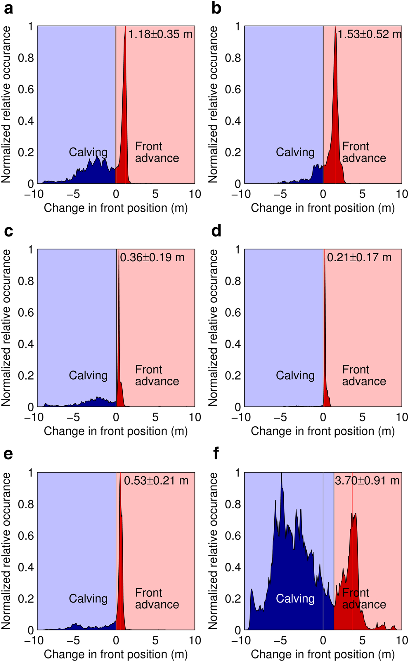
Fig. 4. Histograms of the changes of ice front position of Fuerza Aérea Glacier between 21 January and 04 February 2013. (a) 21–25 January, (b) 25–31 January, (c) 31 January–01 February, (d) 01–02 February, (e) 02–04 February, (f) 21 January–04 February.
Table 1. Ice front position changes, ice flow velocities and calving rate of Fuerza Aérea Glacier measured with TLS over the period 21 January – 04 February 2013

Figure 5 shows the changes in ice front position as measured by the point cloud differentiation, so that a positive change corresponds to frontal advance and negative change to frontal retreat. The ice front position was changing throughout the study period, with a pronounced advance on the left side of the cliff and a retreat associated with calving over the rest of the cliff (Fig. 5). The ice front advance in areas where no calving occurred between measurements is presented in Figure 6. Then, ice front retreat due to calving (Fig. 7) was calculated by subtracting the mean ice flow velocity estimated using the histograms (Fig. 4) from the respective ice front position change map (Fig. 5).
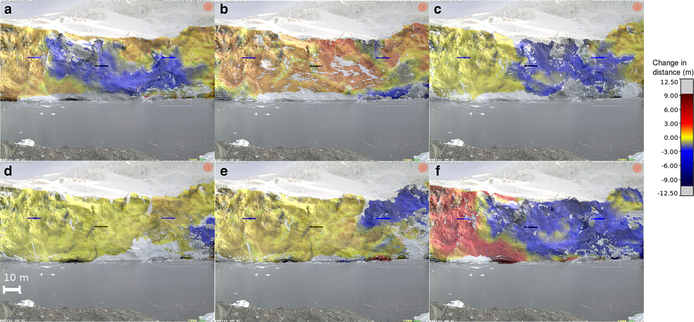
Fig. 5. Changes in the ice front position of Fuerza Aérea Glacier measured with TLS between 21 January and 04 February 2013. (a) 21–25 January, (b) 25–31 January, (c) 31 January–01 February, (d) 01–02 February, (e) 02–04 February, (f) 21 January–04 February.
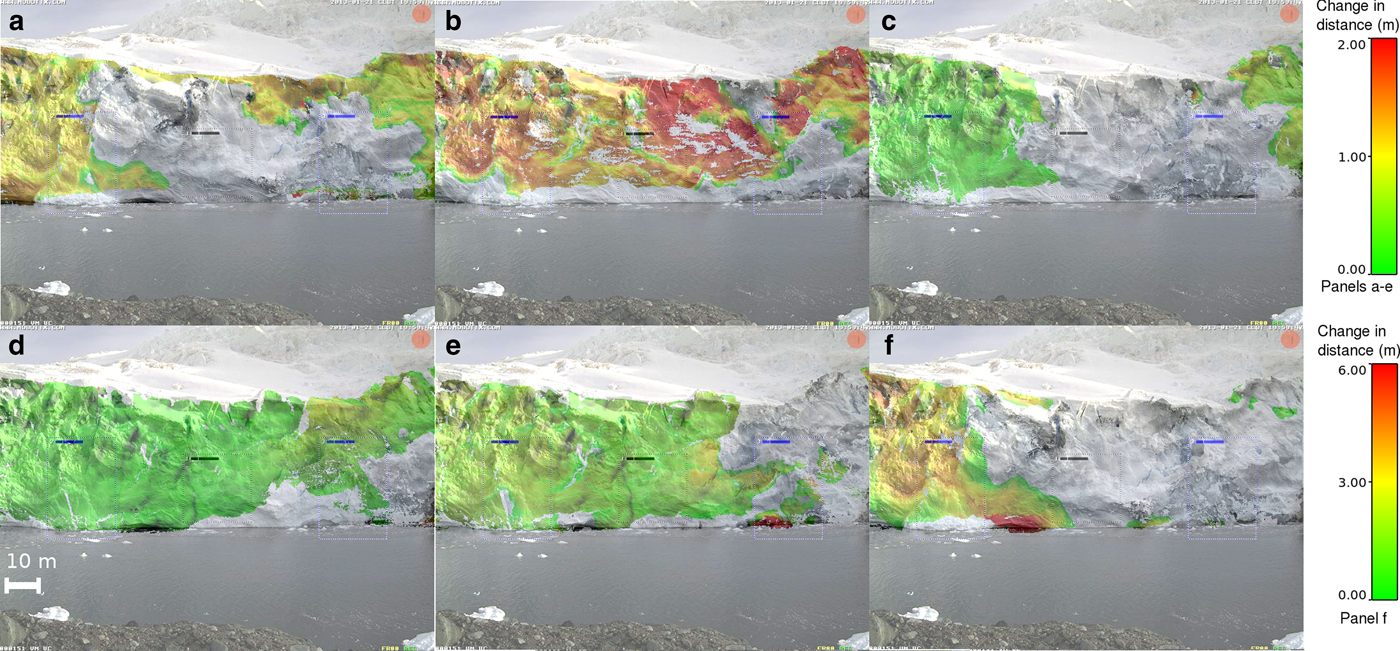
Fig. 6. Ice front advance of Fuerza Aérea Glacier in the areas where no calving occurred, measured with TLS between 21 January and 04 February 2013. (a) 21–25 January, (b) 25–31 January, (c) 31 January–01 February, (d) 01–02 February, (e) 02–04 February, (f) 21 January–04 February. Note the different color scale on panel (f).
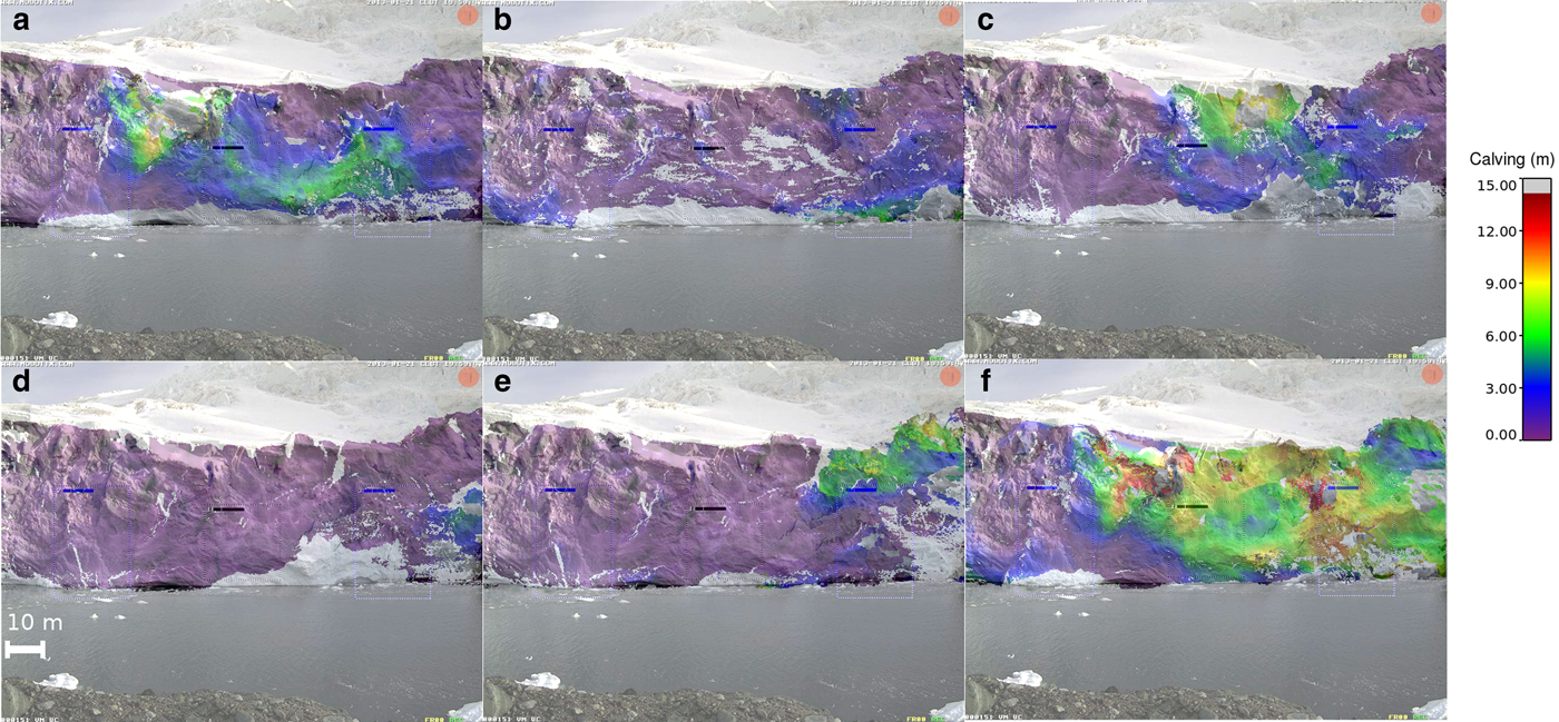
Fig. 7. Calving at the ice cliff of Fuerza Aérea Glacier between 21 January and 04 February 2013. (a) 21–25 January, (b) 25–31 January, (c) 31 January–01 February, (d) 01–02 February, (e) 02–04 February, (f) 21 January–04 February.
The position changes were relatively small, ranging from −9 to +2 m over 2 weeks, resulting in an overall mean front retreat of 2.07 ± 0.19 m (Table 1). Much larger values were recorded where the fallen ice accumulated in shallow water; this is clearly seen in Figures 5e, f. At the beginning of the observations (21–25 January), the negative ice position changes were concentrated in the centre of the ice cliff (Fig. 5a), reaching values of −9 m, whereas the lateral parts advanced (Fig. 6a). The lengths of the calved ice, normal to the ice front, were ~3–6 m (Fig. 7a). During the next observation period (25–31 January, Figs 5b, 6b) almost the entire ice cliff advanced, with a mean position change of 0.83 ± 0.25 m (Table 1). There was some calving activity in the right part of the cliff (Fig. 7b). The next day (31 January–01 February) extensive calving activity was observed (Fig. 7c), resulting in substantial retreat (1.38 ± 0.17 m; Table 1; Fig. 5c) despite the fact that the maximum ice flow velocity of 0.36 ± 0.19 m d−1 occurred on this day (Table 1). Following that, on 01–02 February, almost no calving occured (Fig. 7d) and the entire ice front advanced (Fig. 6d), resulting in a positive mean front position change of 0.11 ± 0.15 m (Table 1; Fig. 5d). During the last period of measurements, calving took place only in the upper right corner of the ice cliff (Fig. 7e). As mentioned, some of the fallen ice could be clearly identified (Fig. 5e) grounded in shallow water. The overall change in ice front position is presented in Figure 5f, where two distinct features can be distinguished: an advance on the left side of the cliff due to ice flow advection undisturbed by calving (Fig. 6f), and large, homogeneous retreat elsewhere caused by several calving events of different sizes (Fig. 7f). There are some discrepancies between Figures 6f and 2b, concerning areas not affected by calving, especially in the left side of the cliff. It seems that the calved ice block that can be seen in the left edge of the cliff was of small length in comparison with the ice front advance over the entire investigated period and therefore was not detected. However, during a shorter observation period it was properly detected, as it can be seen in Figures 6b and 7b.
Even though a clear linear relationship between the measured calving rate and the ice flow velocity at the terminus can be seen in Figure 8, the associated errors of both variables are high (Table 1) and the number of points used is low. Nonetheless, the correlation coefficient is high (R 2 = 0.88) and there are no outliers, indicating a possible link between the ice flow velocity and calving rate.
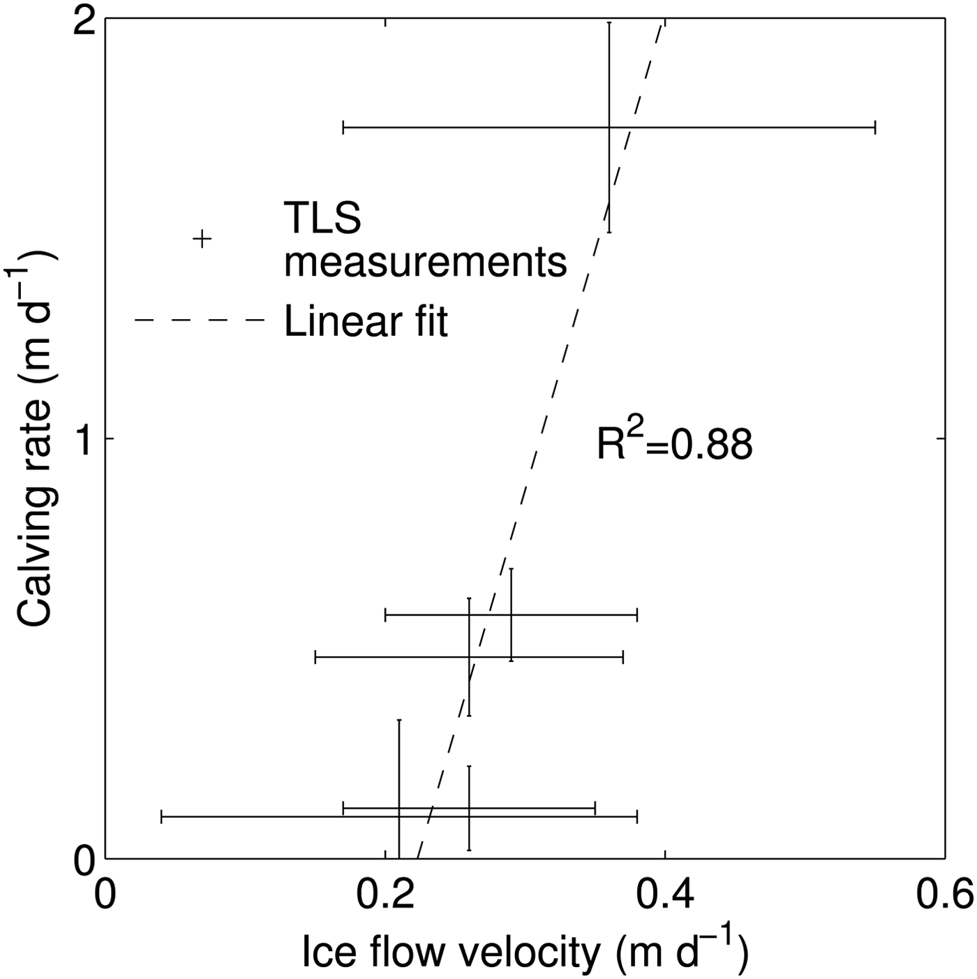
Fig. 8. Scatter plot of calving rate and ice flow velocity of Fuerza Aérea Glacier between 21 January and 04 February 2013.
4.3. Area/volume scaling
In total, nine non-overlapping calving events, spread over the entire ice cliff surface, were identified both in the video monitoring and the laser scans. They had a total volume of 9471 m3, ranging from 0.29 to 5821 m3 (Fig. 9; Table 2). Their area ranged from 961 to 42 592 pixels as measured from the video recording and 1.53–1358 m2 as measured with TLS. A fit to these values (Eqn. (1); Figs 9a, d) was then applied. The volume measurement error was large, especially for smaller calving events (Table 2). The standard deviation of the residuals of fit and observed volumes was low (Figs 9c, d), which can be explained by the small number of large calving events having a large influence on the parameters of the fit. Thus, the error of the fit was set to equal the mean percentage measurement error of the three largest calving events, 16%. Afterwards, this relationship was applied to the record of calving events from video monitoring (Fig. 3) resulting in a complete record of calved ice volume (Fig. 10).

Fig. 9. Calving event area/volume scaling. (a)–(c) Area measured with TLS. (d)–(f) Area measured with video monitoring. (c), (f) Scatter plots of measured vs. modelled calving event volume. The error bars show the combined error of volume calculation due to TLS measurement error (point cloud alignment) and ice advection estimation.
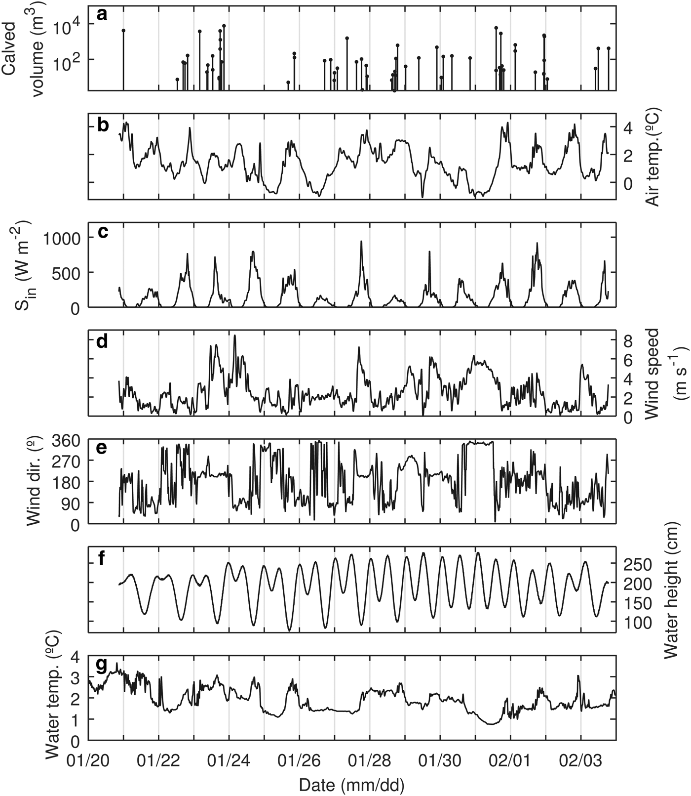
Fig. 10. Calving events and potential environmental drivers recorded during the study period. (a) Calving volume; (b) air temperature; (c) shortwave incoming radiation; (d) wind speed; (e) wind direction; (f) water height; (g) water temperature.
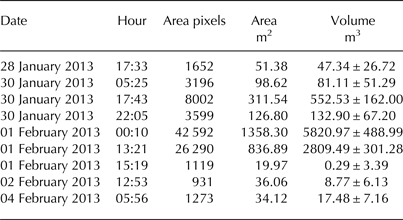
Table 2. Size of nine events that did not occur from the same space on the calving cliff as others during the time interval between TLS measurements. The volume error is calculated as combination of TLS measurement error (point cloud alignment) and ice advection estimation
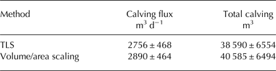
The total volume of calving in the investigated period, obtained by summing all individual calving events, is thus estimated to be 40 585 ± 6494 m3 (Table 3). The direct estimate of calving from TLS results calculated as mean calving rate (Table 1) multiplied by the surface area of the cliff yields 38 590 ± 6554 m3 (Table 3).
Table 3. Calving of Fuerza Aérea Glacier over the period of 21 January – 04 February 2013
5. DISCUSSION
Despite the advantages of the TLS over other surveying methods no detailed study of its application to measurements of calving intensity has so far been published (Chapuis and Tetzlaff, Reference Chapuis and Tetzlaff2014; Pętlicki and others, Reference Pętlicki, Ciepły, Jania, Promińska and Kinnard2015, provide further details). Though the use of TLS is severely limited by its vulnerability to meteorological conditions (especially in polar regions), it can be successfully combined with other methods, such as video monitoring, passive seismics or underwater acoustics, to provide a continuous record of calving volumes. The use of video recording is limited by the availability of sunlight and therefore is not suitable for year-round monitoring in polar regions. However, in such regions it is useful during the period of midnight sun when it can work for 24 h d−1. For this reason, passive seismics and underwater acoustics seem to be the best complementary methods for TLS for long-term monitoring as they are largely independent of light and weather conditions. Nonetheless, their low sensitivity to small volume calving (e.g. O'Neel and others, Reference O'Neel, Larsen, Rupert and Hansen2010; Bartholomaus and others, Reference Bartholomaus2015; Glowacki and others, Reference Glowacki2015) imposes a limit on their applicability to smaller glaciers with low energy calving events. In such instances video recording proves to be a more useful method.
Another advantage of using a video camera over a time-lapse camera is that the whole calving event is captured both with image and sound, allowing for more reliable recognition and mapping. A video record of calving gives insight into the fracture processes that can help classify mechanics (e.g. Bartholomaus and others, Reference Bartholomaus, Larsen, O'Neel and West2012; Glowacki and others, Reference Glowacki2015). The automatic motion detection of the video camera was not a useful tool for calving detection, as the presence of sea birds, changing light conditions and wave action triggered the recording much more often than actual calving. It is worth noting that the calving events that occurred during twilight were identified with the audio recordings that accompanied the video.
A linear relationship between calving rate and ice flow velocity at the terminus was observed (Fig. 8). Similar relationships have been reported before for tidewater glaciers at seasonal to annual timescales (e.g. van der Veen, Reference van der Veen1996), but were not observed at short timescales such as in this study (O'Neel and others, Reference O'Neel, Echelmeyer and Motyka2003). As opposed to the aforementioned studies, the front of Fuerza Aérea Glacier is grounded in very shallow water so that ice flow at the front will not be affected by tidal buoyancy changes. As calving could not be related to any of the potential environmental drivers but was found to be related to ice flow velocity, the ice flow variations themselves must arise from internal glacier processes.
5.1. Probability distribution of calving events
The observed cumulative distribution functions (cdf) of calving event size μ (m3) and inter-event interval τ (min) are shown in Figure 11. The observed distributions were modelled with four commonly used distributions for skewed positive data (power law, exponential, Weibull or ‘stretched exponential’ and log-normal) using the maximum likelihood method. The distributions are compared in Table 4 using the Akaike information criterion (AIC = 2k−2lnL, where L is the maximum value of the likelihood function and k the number of parameters for the distribution). The AIC rewards goodness of fit as assessed by the likelihood function but also penalizes an increase in the number of estimated parameters. A Monte-Carlo Kolmogorov–Smirnov (KS) goodness-of-fit test (Clauset and others, Reference Clauset, Shalizi and Newman2009) was also applied to test the null hypothesis that the observed data follow a hypothesized distribution. Briefly, for each distribution type, 5000 random datasets are generated using the distribution parameters fit to the observed data. Each synthetic dataset is then fit with its own distribution model and the KS statistic is calculated. The p-value corresponds to the fraction of the number of times that the resulting statistic is larger than the value for the empirical data. Following Clauset and others (Reference Clauset, Shalizi and Newman2009), a p-value <0.10 is used to reject the null hypothesis.
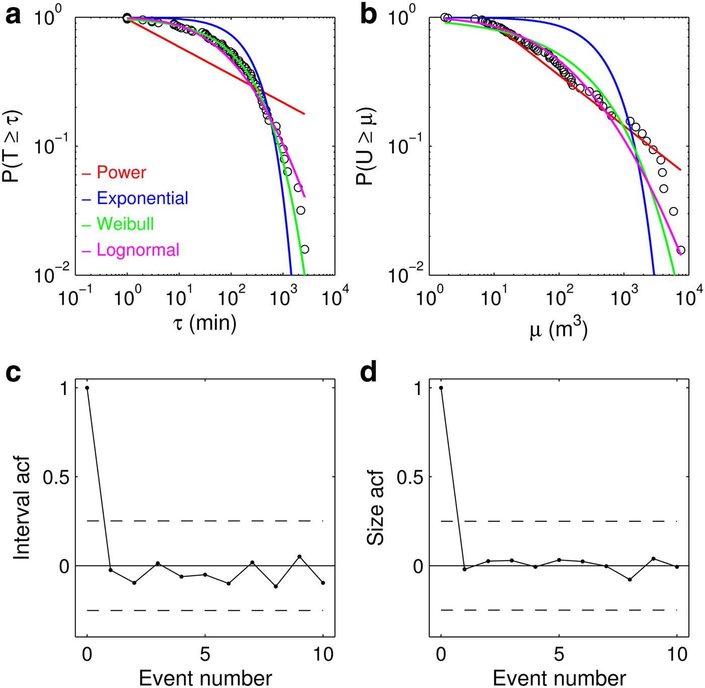
Fig. 11. Cumulative density function (cdf) and autocorrelation (acf) function of calving sizes μ (m3) and interval times τ (min). (a), (b) Observed (circles) and fit (color lines) cdfs for interval times and calving volumes, respectively. (c) Interval acf vs event number. (d) Calving size acf vs event number. Dashed lines in panels (c) and (d) show 95% significance levels.
Table 4. Akaike information criterion (AIC) and p-value of the Kolmogorov–Smirnov (KS) statistic for the theoretical distributions fitted to observed size and inter-event interval data of calving

A p-value <0.10 rejects the null hypothesis that the observed distribution follows a given theoretical distribution.
The simplest model to consider for discrete events such as calving events would be a marked Poisson point process, which implies that calving events occur randomly in time. In this case the inter-event time interval can be shown to be exponentially distributed and independent in time (e.g. Lowen and Teich, Reference Lowen and Teich2005). Neither the power cdf, which has been reported for observed and simulated calving events (Åström and others, Reference Åström2014; Chapuis and Tetzlaff, Reference Chapuis and Tetzlaff2014), nor the exponential cdf fit the interval data well (Fig. 11a) and both also fail the KS test, while the Weibull and log-normal distributions both fit the data better and pass the hypothesis test (Table 4). The assumption of time independence on the other hand is confirmed by the autocorrelation function (acf) plot, which shows insignificant lagged correlations (Fig. 11c). Based on these observations the occurrence of calving events appears to follow neither a simple Poisson process nor a fractal point process with power- law distributed interval times (e.g Lowen and Teich, Reference Lowen and Teich2005). The calving event size distribution (Fig. 11b) is not well fit by any of the distributions considered; only the lognormal distribution passes the hypothesis tests, but with a rather low p-value (Table 4). However, the power-law distribution fits the data well until a cut off near 1.5 × 10 m3 after which the calving probability decreases. The acf function of event sizes shows no memory in the calving process (Fig. 11c).
Åström and others (Reference Åström2014) recently showed that modelled and observed calving fragment size and inter-event interval distributions tend to follow power laws, suggesting that calving exhibits self-organized criticality (SOC; e.g. Lowen and Teich, Reference Lowen and Teich2005). SOC systems have a sub-critical regime distinguished by infrequent and small avalanches, allowing instability to build up with time and a super-critical regime distinguished by large avalanches and widespread relaxation of the conditions (stresses) responsible for the instability. They spontaneously self-organize towards a stable ‘critical point’ between these two unstable regimes, and close to this critical point (the ‘critical region’), the system begins to exhibit scale invariance (Åström and others, Reference Åström2014). They noted that grounded tidewater glaciers in Svalbard and Alaska were best fit by a power law with a cut off at ~104 m, which reflects how calving is limited by the dimensions of the terminus. While Åström and others (Reference Åström2014) present compelling evidence in support of calving behaving as a SOC system, at least one glacier studied by these authors did not exhibit a power-law inter-event interval distribution (Yahtse Glacier; Åström and others, Reference Åström2014, their Supplementary Fig. 3). Chapuis and Tetzlaff (Reference Chapuis and Tetzlaff2014) also showed that inter-event interval distributions are broad but have a less pronounced tail than power laws. Our results are in line with those of Chapuis and Tetzlaff (Reference Chapuis and Tetzlaff2014): while our event size distribution appears to follow a power law with an exponential cut off near 1.5 × 10 m3, the inter-event interval distribution does not follow an exponential model (Poisson process), and also has a less pronounced tail than the power law implied by SOC systems.
5.2. Environmental forcing of calving events
Calving events are represented in Figure 10 along with the different environmental variables recorded during the study period. Elevated temperature and incoming solar radiation could in theory increase the probability of calving, through increased surface melting and resulting infiltration of meltwater in crevasses (Benn and others, Reference Benn, Warren and Mottram2007b). Using the wind speed as a proxy of ocean wave intensity, it might be expected that stronger onshore winds (north to northeasterly in this case) combined with elevated ocean water temperature will favor calving by thermo-erosional undercutting of the ice cliff at the ocean waterline. This has been shown to be an important process for tidewater glaciers (Pętlicki and others, Reference Pętlicki, Ciepły, Jania, Promińska and Kinnard2015). Tidal variations affect buoyancy forces at the glacier front. Decreasing and low tides have been shown to increase ice motion at a glacier front (Sugiyama and others, Reference Sugiyama, Sakakibara, Tsutaki, Maruyama and Sawagaki2015) and to increase calving fluxes (Bartholomaus and others, Reference Bartholomaus2015). However, no simple relationship appears to be visually discernable between the occurrence and volume of calving events and any of the potential environmental drivers. In some, but not all instances of high air temperature, there does appear to be a relation between air temperature and calving volume. Stepwise logistic regression was used to examine whether any additive combination of the variables in Figure 10 could explain the probability of calving event occurrence. Although a significant (p < 0.05) relationship was found with air temperature (positive) and water height (negative), the generalized R coefficient of determination was very low (R 2 = 0.04). Hence, the occurrence of calving events does not seem to be significantly controlled by variations in the recorded environmental parameters, at least at the timescale considered (2 weeks). We also plotted calving volumes against each driver (Fig. 12) and could not find any simple bivariate relation. Stepwise linear regression of calving volume (log-transformed) against the six environmental variables yielded no significant relationships (p > 0.05).
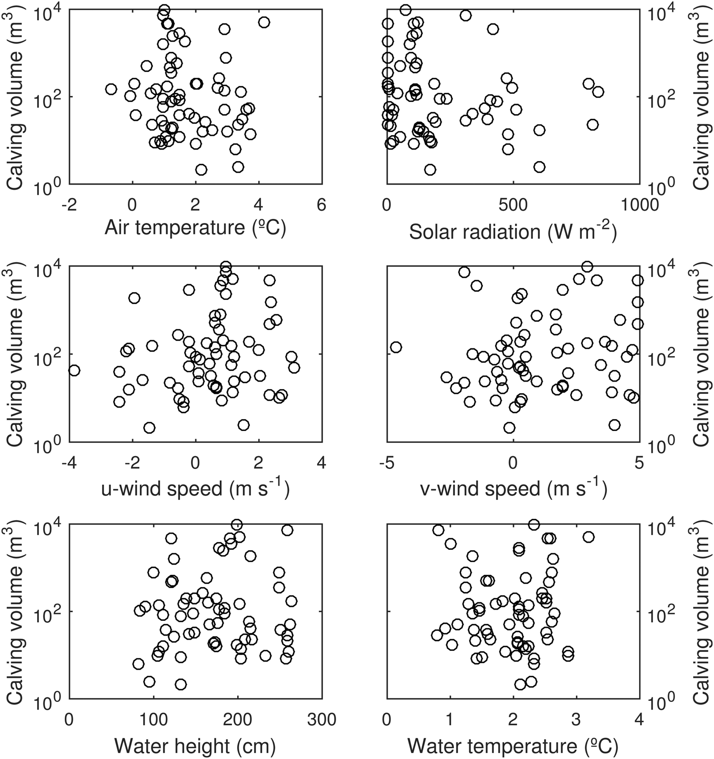
Fig. 12. Bivariate scatterplots of calving volumes against environmental variables. Wind speed convention: positive (negative) u winds are from the west (east); positive (negative) v winds are from the south (north).
Taken together these results support recent findings by Chapuis and Tetzlaff (Reference Chapuis and Tetzlaff2014), who showed that fluctuations in external environmental drivers are not required to explain the event-size and interval variability observed in field data over a 2 week period. While fluctuations in environmental drivers at larger timescale (seasonal and interannual) have been shown to have a clear influence on calving activity (e.g. Åström and others, Reference Åström2014; Luckman and others, Reference Luckman2015), the occurrence and size distribution of calving events at the timescale considered in this study appears to result from internal, perhaps self organized, processes (Åström and others, Reference Åström2014).
6. CONCLUSIONS
We have described a methodology for applying a combination of long-range TLS measurement and continuous video recording to monitor the calving activity of a tidewater glacier. It was successfully applied to short-term (14 d) observations of Fuerza Aérea Glacier. Throughout the observation time, the calving rate varied between 0.10 ± 0.23 and 1.74 ± 0.25 m d−1, with a mean value of 0.41 ± 0.07 m d−1. In total, 64 calving events of different size were identified, of which nine that did not occur from the same space on the calving cliff as others during the time interval between measurements were used for calving event area/volume scaling. The calving event size distribution is best approximated by a power-law distribution with a cut-off frequency at 1.5 × 10³ m3. For the time span of the observations no clear relationship was found between the environmental forcings and calving activity, but calving was positively related to ice flow velocity. Therefore calving over such a short period of time appears to be governed by ice dynamics and seems to be an internal process of the ice front.
ACKNOWLEDGMENTS
We thank Sandro Zambra for valuable help in processing of video data, Jakob Abermann for his help in collection of data and the staff of Chilean Navy Antarctic Base Arturo Prat for logistic support during field work. This study was funded by the Chilean National Antarctic Institute (INACH) grant RT12_12 and, within statutory activities, Grant No. 3841/E-41/S/2016 of the Ministry of Science and Higher Education of Poland. The publication has been partially financed by the Centre of Polar Studies from the funds of the Leading National Research Centre (KNOW) received for the period 2014–2018. We thank reviewers Ryan Cassotto and Roger LeB. Hooke for helpful comments.


 Open access