Introduction
Low temperatures, low snow accumulation and a surface climate dominated by near-continuous, dry inversion-driven airflow leads to a complex interaction between snow, wind and topography on the East Antarctic ice sheet (EAIS) plateau. This interaction has important effects on the local surface net mass balance in undulating regions of the ice sheet (areas having topography of one to tens of meters relief, at horizontal scales of a few hundred meters to a few tens of kilometers). Features such as megadunes, snow-glaze areas and local accumulation highs are manifestations of this interaction typical of East Antarctica (Reference Fahnestock, Scambos, Shuman, Arthern, Winebrenner and KwokFahnestock and others, 2000; Reference Frezzotti, Gandolfi, La Marca and UrbiniFrezzotti and others, 2002a,Reference Frezzotti, Gandolfi and Urbinib). This wind- topography interaction creates a continuum of snow erosional/depositional effects that control blue-ice exposure as well as local (~10km scale and less) accumulation rates for the West Antarctic and Greenland ice sheets (e.g. Reference GoodwinGoodwin, 1990; Reference Hoen and ZebkerHoen and Zebker, 2000; Reference Winther, Jespersen and ListonWinther and others, 2001;Reference King, Anderson, Vaughan, Mann, Mobbs and VosperKing and others, 2004;Reference Van de Berg, Van den Broeke, Reijmer and Van MeijgaardVan den Broeke and others, 2006), and probably grade into some aspects of snow redistribution on ice fields and smaller ice caps.
Most of the Antarctic ice sheet has a snow/firn cover of about 70-100m thickness, transitioning with depth into ice. In blue-ice areas, ice is exposed on the surface and there is no covering of firn/snow. This is because wind and sublimation can ablate much more snow/firn than is accumulated by annual solid precipitation, causing a persistent strong negative surface mass balance (SMB) that removes the firn. Blue-ice areas occur in mountainous regions and at katabatic wind confluence areas in steeply sloping and near-coastal regions. Exposed blue ice covers ~1% of the Antarctic ice sheet (Reference Winther, Jespersen and ListonWinther and others, 2001). Ablation rates in blue-ice areas decrease with increasing distance from the ice-sheet edge, with negative values of SMB from -500 to -30 kg m-2 a-1 (Reference Bintanja and Van den BroekeBintanja and Van den Broeke, 1995). In contrast, wind-glazed areas are regions where wind and sublimation removes about the same amount as the annual solid precipitation total, creating a hiatus in accumulation as the surface ice flows across the wind-glazed area. Their SMB is close to nil (-20 to 20 kgm-2 a-1).
Wind-glazed areas are far more extensive on the EAIS surface than blue ice, as we show in this study. The primary characteristic of wind-glaze surfaces from the perspective of this study is their near-zero SMB, which leads to distinctive surface and subsurface characteristics that can be mapped from space. Because the regions have been largely unrecognized and are generally too small to be resolved by climate models, their presence represents local lows in accumulation estimates that are not represented in current surface mass-balance grids. We review the characteristics and formation of wind-glaze regions from published literature and supporting field observations conducted for this study. We then discuss the satellite remote-sensing measurements we use to conduct an EAIS-wide mapping of wind-glaze regions, and present the mapped extent. Finally, we estimate the net effect of the regions on past estimates of snow accumulation on the EAIS. The presence of wind glaze over a significant fraction of the high EAIS surface leads to a significant revision of the total mass input to East Antarctica. This impacts mass-balance estimates based on the mass budget approach.
Field Characteristics of Wind-Glaze Regions
Wind-glaze areas are irregular to elongated patches of a few hundred meters to a few tens of kilometers in linear dimensions, characterized by a wind-polished glazed surface overlying a coarsely recrystallized firn layer (Fig. 1a; Wantanabe, 1978;Reference GoodwinGoodwin, 1990;Reference Frezzotti, Gandolfi, La Marca and UrbiniFrezzotti and others, 2002a;Reference Albert, Shuman, Courville, Bauer, Fahnestock and ScambosAlbert and others, 2004). They occur almost exclusively in East Antarctica. The features are observed generally above ~1500 m elevation as well as in confluence areas of katabatic winds (e.g. David Glacier, Mertz-Cook catchment basins) (Reference Scarchilli, Frezzotti, Grigioni, De Silvestri, Agnoletto and DolciScarchilli and others, 2010), and up to within a few tens of kilometers of the EAIS ice divide at 3600-3800m elevation (Reference WatanabeWatanabe, 1978; this study). Wind polishing by blowing snow occurs primarily from autumn to early spring (Reference Scarchilli, Frezzotti, Grigioni, De Silvestri, Agnoletto and DolciScarchilli and others, 2010), when katabatic wind speed and persistence is greatest (Reference Parish and BromwichParish and Bromwich, 1987). The polished glaze surface transmits more solar energy into the underlying firn than an unmodified snow surface, allowing solar radiation to penetrate and warm the subsurface layer. This in turn drives a greater upward transport of water vapor, followed by condensation of the vapor against the underside of the glaze surface. Reference Fujii and KusunokiFujii and Kusunoki (1982) showed that this underplating of the surface crust occurred between August and January, caused by vapor transport and condensation. The process is slow during winter months, but increases during late spring and summer due to higher vapor pressure as the firn temperature increases.

Fig. 1. Surface and subsurface characteristics of wind-glaze regions in East Antarctica. (a) Wind-glaze region near 82° S, 110° E (near TAMSeis Camp) on 23 November 2002, showing bright forward scattering of wind-polished snow surface. (b) Backlit snow-pit photograph in wind-glaze region between megadunes, showing coarse recrystallized grains (80.24° S, 124.5° W, Megadunes Camp, January 2004); centimeter scale is shown on left side of image. (c) Thermal(?) cracks typical of permanent wind-glaze areas (X-shaped pattern of fine ridges in foreground) at 84.2° S, 20.7° E on 4 January 2009. (d) Wind-glaze area near 88.1° S, 2.2° W on 25 December 2008. (e) Typical sastrugi patterns adjacent to wind-glaze areas (few km south of (c)). (c-e) photographs taken during Norway-US International Polar Year (IPY) Science Traverse, 2008/09 season.
During late spring and summer, the large temperature gradient between the solar-heated surface layer and colder firn at depth also causes extensive depth-hoar formation (Fig. 1b; Reference Albert, Shuman, Courville, Bauer, Fahnestock and ScambosAlbert and others, 2004;Reference Courville, Albert, Fahnestock, Cathles and ShumanCourville and others, 2007). This creates coarse (~0.5 to 1.0 cm) cup-shaped ice crystals (e.g. Reference DenHartogDenHartog, 1959; Reference GiovinettoGiovinetto, 1963; Reference Goodwin, Higham, Allison and RenGoodwin and others, 1994; Reference Gay, Fily, Genthon, Frezzotti, Oerter and WintherGay and others, 2002; Reference Courville, Albert, Fahnestock, Cathles and ShumanCourville and others, 2007). Repeated seasonal thermal cycling of the upper firn with low or zero accumulation results in a several meters thick layer of these coarse recrystallized grains, with almost no remnant of layering or depositional density variations remaining (as in Fig. 1b). Repeated thermal cycling also leads to the formation of surface cracks, presumably by thermal expansion and contraction of the upper snow/firn layer (Fig. 1c; Reference WatanabeWatanabe, 1978; Reference Frezzotti, Gandolfi, La Marca and UrbiniFrezzotti and others, 2002a; Reference Albert, Shuman, Courville, Bauer, Fahnestock and ScambosAlbert and others, 2004; Reference Courville, Albert, Fahnestock, Cathles and ShumanCourville and others, 2007). These cracks are several meters deep and divide the surface into irregular polygons a few meters across. In late summer, radiative cooling of the uppermost surface layer leads to formation of a surface frost, by condensation of local atmospheric vapor onto the snow surface (e.g. Reference Shuman and AlleyShuman and Alley, 1993). This gives the glaze surface a more diffuse specular reflection than in spring (Fig. 1d), and changes its appearance in remote-sensing data. Late-summer/early-fall surface frost formation is widespread, and not exclusively associated with wind glaze.
Formation of wind-glaze surfaces appears to result from locally increased average inversion wind speed due to an increase in local surface slope in the downwind direction (Reference Frezzotti, Gandolfi, La Marca and UrbiniFrezzotti and others, 2002a). Because inversion flow is a gravity-driven drainage of a cold inversion air layer, an increase in surface slope over a distance of a few times the inversion layer thickness (typically ~100-300 m; Reference ConnolleyConnolley, 1996) can accelerate the flow. Increased wind speeds lead to an increase in blowing-snow transport, and an increase in surface and within-airstream sublimation of snow due to adiabatic heating and compression (e.g. Reference Neumann, Waddington, Steig and GrootesNeumann and others, 2005; Reference Scarchilli, Frezzotti, Grigioni, De Silvestri, Agnoletto and DolciScarchilli and others, 2010), that over the annual cycle removes all or almost all of the precipitated or wind-deposited snow that may temporarily accumulate. Instrumental observations integrated with a snow accumulation survey (snow radar, firn core, remote sensing) suggest that the combined processes of blowing-snow sublimation and snow transport remove up to 50% of precipitation in some coastal and slope convergence areas (Reference Scarchilli, Frezzotti, Grigioni, De Silvestri, Agnoletto and DolciScarchilli and others, 2010). However, armoring of the surface by the wind-glaze crust prevents significant ablation of the surface over a range of moderate wind speeds. For example, glazed surfaces (and not blue ice) are widespread in the David Glacier and Lambert Glacier basins where mean wind speeds are >11 m s-1 during most of the year (Reference Goodwin, Higham, Allison and RenGoodwin and others, 1994; Reference FrezzottiFrezzotti and others, 2005). Field measurements in regions of wind glaze show few areas of significant negative SMB (e.g. Japanese Antarctic Research Expedition (JARE); see Fig. 2; Reference MotoyamaMotoyama and others, 2008).

Fig. 2. Mean snow accumulation from the JARE stake line, 1993-2007 (14 years) for stations S16 to MD738 converted to net SMB assuming a snow density of 350kgm-3. Profiles along the stake line from four recent regional net surface mass-balance estimates are shown for comparison. Dashed line shows the surface mass-balance threshold for glaze extent used in this study, 20 kg m-2 a-1.
In regions adjacent to wind-glaze surfaces, as wind- direction surface slope flattens or even reverses, a local high in accumulation may occur in the form of a large transverse dune or series of dune/glaze pairs. For a narrow range of wind-direction slopes, the alternation between transverse glaze stripes and accumulating ridges can become self-reinforcing, leading to long trains of glaze- dune pairs called megadunes. In this case, the accumulation stripe modifies the regional mean slope such that the accreting face is relatively flat or reversed with respect to the wind direction, and the back side steepens to the point of supporting faster local winds and therefore glaze formation. Accumulating surfaces are generally rough (Reference WatanabeWatanabe, 1978; Reference GoodwinGoodwin, 1990; Reference Fahnestock, Scambos, Shuman, Arthern, Winebrenner and KwokFahnestock and others 2000; Fig. 1e) with well-sintered fine-grained snow in complexly eroded sastrugi forms. Wind-glaze areas are very flat and smooth, with few if any sastrugi forms. Thus, the differences in surface texture amplify the accumulating nature of the dune stripes and the reduced accumulation of the glaze areas, as the near-surface blowing snow interacts with these distinct roughness variations.
The accumulation areas can in part offset the local low in accumulation represented by the glaze surface. However, at two megadune field sites, 81.24° S, 124.5° E and 75.5° S, 129.5° E (Reference Frezzotti, Gandolfi, La Marca and UrbiniFrezzotti and others, 2002b; Reference Albert, Shuman, Courville, Bauer, Fahnestock and ScambosAlbert and others, 2004; Reference Scambos, Fahnestock, Shuman and HaranScambos and others, 2006), and over long-term snow stake fields (e.g. JARE and the Chinese Antarctic Research Expedition (CHINARE) (Reference MotoyamaMotoyama and others, 2008; Reference DingDing and others, 2011)), the adjacent accumulation highs do not compensate for the near-zero glaze region extent relative to regional accumulation estimates or nearby field measurements (e.g. JARE line; Fig. 2). At the megadune field site, two accumulation measurements using β-radiation detection of nuclear bomb fallout in shallow firn cores were made near the highest-accumulation portion of the dune crests. The measured values (33.5 and 42.0 kgm-2 a-1) are at or below the accumulation value attributed to the entire region (glaze and dune crest together) for several recent continent-wide SMB models (Reference Arthern, Winebrenner and VaughanArthern and others, 2006; Reference Monaghan, Bromwich and WangMonaghan and others, 2006; Reference Scambos, Fahnestock, Shuman and HaranScambos and others, 2006; Reference Van de Berg, Van den Broeke, Reijmer and Van MeijgaardVan de Berg and others, 2006; Reference Courville, Albert, Fahnestock, Cathles and ShumanCourville and others, 2007). However, for both the JARE line and the megadune field sites, the recent RACMO2 Antarctic regional atmospheric climate model (Reference Lenaerts, Van den Broeke, Van de Berg, Van Meijgaard and Kuipers MunnekeLenaerts and others, 2012) is closer to the net total SMB as measured (~20 kg m-2 a-1; Fig. 2). We consider the estimates of these SMB models for wind-glaze areas over the entire EAIS.
While the glaze formation processes can occur for short periods in a net accumulation environment, creating a temporary wind-glaze surface, it is the long-term (decades to centuries) lack of accumulation and the persistence of a steady and locally increased katabatic flow in the steeper windswept areas that leads to extreme development of these characteristics in the near-surface firn layer. Persistence of wind intensity and direction in the EAIS is very high between 1500 and 3500 m elevation (Reference Parish and BromwichParish and Bromwich, 1987; Reference Fahnestock, Scambos, Shuman, Arthern, Winebrenner and KwokFahnestock and others, 2000). Although katabatic airflow patterns can dominate wind conditions in lower-elevation regions as well, intervals of cyclonic-driven winds and increased snowfall lead to a mix of surface conditions at a given site. This results in less consistent (temporally intermittent) wind-glaze surfaces, with higher net accumulation and therefore less development of recrystallized firn and an absence of thermal cracks (Reference GoodwinGoodwin, 1990).
The near-zero net accumulation of wind-glaze areas has been shown in numerous studies, most effectively by regional stake-line surveys and ground-penetrating radar (GPR) profiles. Although temporary accumulation events can occur on glaze surfaces, appearing as scattered low-relief sastrugi, these are transient on the multi-annual scale (Reference MotoyamaMotoyama and others, 2008). Other means of determining net accumulation (e.g. snow-pit studies of firn layering, or isotopic-based determinations) often yield uninterpretable or misinterpreted results (e.g. Reference Rundle and CraryRundle, 1971). Both firn layering and isotopic variation within the ice are blurred or erased by the intense firn recrystallization. Thus past accumulation compilations from interpolation of field measurements (Reference Vaughan, Bamber, Giovinetto, Russell and CooperVaughan and others, 1999;Reference Giovinetto and ZwallyGiovinetto and Zwally, 2000;Reference Arthern, Winebrenner and VaughanArthern and others, 2006) using remote-sensing data had few valid near-zero accumulation measurements in the East Antarctic, and therefore likely interpolated across important regions of lower (near-zero) accumulation represented by wind-glaze regions. It is likely that the source datasets for the SMB compilations may have treated some sites with valid nearzero accumulation results as 'missing data' (e.g. due to inconclusive β-radiation methods, snow-pit or shallow-core layering assessments, annual chemistry or isotope variations).
The recent version of RACMO2 used by Reference Lenaerts, Van den Broeke, Van de Berg, Van Meijgaard and Kuipers MunnekeLenaerts and others (2012) accounts for the sublimation and erosion/ deposition effects of drifting snow and increased katabatic airflow in increased slope areas. As we present below, however, these locally increased surface slopes are generally smaller in spatial scale than the true resolution of current continent-wide digital elevation models (DEMs) (~5 km (e.g. Reference Bamber, Gomez-Dans and GriggsBamber and others, 2009); ~10km (Reference Liu, Jezek and LiLiu and others, 1999)) or RACMO2 (currently 27 km grid spacing).
Remote-Sensing Datasets and Measurement Errors
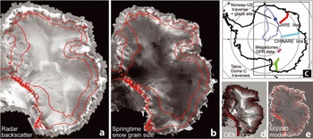
We exploit the distinctive surface and subsurface character of glaze regions to map their extent at ~125m resolution over the entire EAIS plateau above 1500 m (World Geodetic System 1984 (WGS84) datum). Our investigation is limited to elevations above 1500 m because the area below this elevation has extensive crevassing and occasional surface melting that affects radar backscatter from satellite data (e.g. Reference Magand, Picard, Brucker, Fily and GenthonMagand and others, 2008). The two main datasets used for the mapping are C-band imaging radar backscatter from the RADARSAT-1 Antarctic Mapping Project (RAMP) and mean springtime surface optical snow grain size derived from Moderate Resolution Imaging Spectroradiometer (MODIS) data (Fig. 3a and b). To determine thresholds for the wind- glaze mapping algorithm, we use five sets of extensive, near- continuous field measurements of SMB: (1) the Norway-US Scientific Traverse of East Antarctica GPR profiles (Reference MüllerMüller and others, 2010); (2) the JARE repeat snow stake-line measurements between 1993 and 2007 (503 stakes for 14 seasons; Reference MotoyamaMotoyama and others (2008) and other references in the JARE data report series); (3) the CHINARE repeat snow stake-line measurements (528 sites, measured four times over 1997-2008; Reference DingDing and others, 2011); (4) GPR profile estimates from the megadune field site near 80.24° S, 124.5° W crossing two β-radiation measurements (Reference Scambos, Fahnestock, Shuman and HaranScambos and others, 2006;Reference Courville, Albert, Fahnestock, Cathles and ShumanCourville and others, 2007); and (5) GPR- determined accumulation from a set of traverses and ice cores near Talos Dome (Reference FrezzottiFrezzotti and others, 2005, Reference Frezzotti, Urbini, Proposito, Scarchilli and Gandolfi2007). Locations of the field accumulation measurements are shown in Figure 3c.

Fig. 3. Overview of datasets used for wind-glaze mapping. Study area is the region above 1500 m within the EAIS subscenes of RAMP backscatter (a) and MOA-derived springtime surface grain size (b). Red contours are 1500 and 2500 m elevation. (c) Locations of the field data used to develop the mapping relationship. (d) Absolute surface slope of the Reference Bamber, Gomez-Dans and GriggsBamber and others (2009) DEM dataset. (e) MSWD is surface slope in the annual mean wind direction, with surface slope determined from the Reference Bamber, Gomez-Dans and GriggsBamber and others (2009) DEM dataset and annual mean wind direction determined from the RACMO2/ANT model (Reference Lenaerts, Van den Broeke, Van de Berg, Van Meijgaard and Kuipers MunnekeLenaerts and others, 2012).
The radar backscatter dataset of the Antarctic continent has been described previously (Fig. 3a; Reference JezekJezek, 2003). It is derived from a dedicated data collection campaign in September-October 1997 by the RADARSAT-1 C-band satellite synthetic aperture radar (SAR) system, having an original resolution of 25 m. This was re-processed to a 125 m normalized backscatter image with a nominal radar incidence angle of 27° (the center-swath incidence angle of the beam mode used for the majority of the continent). Residual speckle in the 125 m image, and seams due to imperfect normalization of the incidence angle, lead to a noise level of ±1.1 dB (1σ, estimated from the grid value standard deviation after 2 km spatial scale high-pass filtering).
The near-radial pattern of the majority of the swath acquisitions for the RAMP Antarctic Mapping Mission-1 (AMM-1) data (Fig. 3a) means that the viewing direction crosses a broad range of mean wind and surface slope azimuths. Azimuthal variations in radar backscatter with respect to wind and slope over the EAIS can be significant, and appear to be consistent over time and geographical regions (Reference Long and DrinkwaterLong and Drinkwater, 2000). These variations arise from changes in scattering intensity of sastrugi as the incidence direction changes from the along-wind to across-wind direction (Reference Suhn, Jezek, Baumgartner, Forster, Mosley-Thompson and SteinSuhn and others, 1999), probably due to wind crust and density layer orientations. In some regions, variations are 4-8 dB (Reference Suhn, Jezek, Baumgartner, Forster, Mosley-Thompson and SteinSuhn and others, 1999; Reference Long and DrinkwaterLong and Drinkwater, 2000). However, a study comparing regions with a high percentage of wind glaze (two megadune areas) with an adjacent region that is glaze-free showed that backscatter modulation dropped significantly in the megadune regions (Reference Lambert and LongLambert and Long, 2006). Moreover, wind- glaze areas are characterized by very sparse, low-relief sastrugi and intense subsurface recrystallization. Subsurface recrystallization textures show no variation with direction (e.g. Reference Courville, Albert, Fahnestock, Cathles and ShumanCourville and others, 2007;Fig. 1b), and surface thermal(?) cracking is also apparently random in orientation; thus we expect little azimuthal backscatter variation in glaze areas.
Surface grain size is mapped using a normalized bandratio of the two highest-resolution bands in MODIS band 1 (at 670 and 2800 nm, both with 250 m nominal resolution; Fig. 3b), with atmospheric and snow reflectance variations corrected. The band-ratio approach is based on the increased absorption of infrared light in coarser-grained ice and snow (Reference Nolin and DozierNolin and Dozier, 2000; Reference Warren and BrandtWarren and Brandt, 2008). Reference Scambos, Haran, Fahnestock, Painter and BohlanderScambos and others (2007) created a summer mean surface snow grain-size map of the entire Antarctic ice sheet for the 2003/04 season as part of the MODIS Mosaic of Antarctica (MOA) datasets using the same atmosphere-corrected bandratio technique we use here. For this study, we used image data from mid- to late spring only, including additional early- spring images not used in the MOA compilation. We also created a new MOA-style mosaic and grain-size image for a second spring season, in late 2008. The two springtime mean optical surface snow grain-size mappings were found to emphasize the grain-size contrast between wind-glaze regions and adjacent areas relative to the spring-summer composites. We accumulated image data from over 120 MODIS scenes in each of two austral spring seasons (2003 and 2008, each spanning 5 November to 20 December) and composited the data similarly to the MOA. Sub-pixel compositing improves spatial resolution to 150-200m (Reference Scambos, Haran, Fahnestock, Painter and BohlanderScambos and others, 2007). We used the gridcell average value of the two grain-size mappings for the wind-glaze area determination.
Mapping of spring surface optical snow grain size for 2 years allows for some characterization of the interannual variability of this parameter for the study region, and provides a rough estimate of the error of the grain-size measurements. Both snow grain-size mappings show very consistent continent-wide patterns. Grain size is low (~50mm) in near-coastal areas having high accumulation; moderate (50-80 mm) near the ice-divide areas; and larger (80-400mm) for areas of steep slope, including extensive and distributed small wind-glaze areas, blue-ice areas and regions near nunataks and outlet glacier troughs. Mean difference between the two determinations is 10.0 ± 27.3 mm (slightly coarser overall in 2008) for the East Antarctic study area above 1500 m. Regionally, there were differences of typically ±40mm (maximum of ±80mm for ~10 000km2 areas). The largest region with a significant snow grain-size change is the eastern flank of the Amery- Lambert basin, particularly in the Grove Mountains area. This region shows smaller 2008 grain size by ~50 µm relative to 2003. This variation may have impacted the CHINARE traverse results, as we discuss below. Higher 2008 grain size is observed in the Byrd Glacier catchment basin and eastern Wilkes Land. Grain size was relatively unchanged (<20µm difference) in Dronning Maud Land, central Wilkes Land and near South Pole. We estimate local measurement noise to be ±18 mm (1σ), derived from the histogram of a high-pass filtered version (2 km equivalent filter scale) of the two-season averaged 125 m snow grain- size image. However, this measurement error does not account for the interannual variability among regions, and our two mappings of grain size provide only an approximate scale for this.
Field-based studies have made a strong case that mean slope in the (mean) wind direction (MSWD) controls SMB and the formation of wind-glaze regions in the high East Antarctic plateau (Reference Fahnestock, Scambos, Shuman, Arthern, Winebrenner and KwokFahnestock and others, 2000; Reference FrezzottiFrezzotti and others, 2005, Reference Frezzotti, Urbini, Proposito, Scarchilli and Gandolfi2007) through a local increase in mean katabatic wind speed. We created a grid of MSWD from the dot product of an absolute slope field derived from a recent high-resolution elevation model (Fig. 3d; Reference Bamber, Gomez-Dans and GriggsBamber and others, 2009) and a model-derived estimate of annual mean wind direction (from the RACMO2/ANT model;Reference Van de Berg, Van den Broeke, Reijmer and Van MeijgaardVan de Berg and others, 2006; Reference Lenaerts, Van den Broeke, Van de Berg, Van Meijgaard and Kuipers MunnekeLenaerts and others, 2012). The MSWD grid was created at 125 m resolution in the same projection as the remote-sensing data, for ease of comparison (Fig. 3e), although the true resolution is significantly larger (5-8 km).
Remote-sensing characteristics of the field SMB datasets
The field-gathered SMB datasets we use to develop the mapping algorithm are selected to be continuous or near- continuous, each spanning a significant extent on the EAIS plateau, over a large latitude range within the dry snow zone and widely distributed across the study region (Fig. 3c). We selected GPR and snow stake data because these SMB data types can reliably indicate low, zero or slightly negative SMB, an important quality for wind-glaze mapping. (β-radiation horizons, shallow core or pit layering, or oxygen-isotope- based SMB estimates are prone to errors or misinterpretation in wind-glaze regions; see Reference Courville, Albert, Fahnestock, Cathles and ShumanCourville and others, 2007; Reference MagandMagand and others, 2007.)
The JARE traverse spans a large elevation and accumulation range, and its persistent low-accumulation sites are used to identify the major remote-sensing characteristics of the wind-glaze features relative to surrounding higher- accumulation surfaces. Local accumulation lows in the stake-line data are consistently associated with higher surface optical grain size, higher backscatter and lower surface roughness compared to adjacent stake areas (Fig. 4). We use surface grain size in particular to identify local wind- glaze areas relative to surroundings. Although surface roughness appears to be a further robust defining characteristic, with wind-glaze regions being significantly smoother than surrounding terrain (lowest graph in Fig. 4), further work is needed on a satellite-based roughness mapping algorithm to make it quantitative and uniform across the ice sheet. (We are evaluating a normalized ratio of the C fore- and aft- viewing cameras on the Multi-angle Imaging SpectroRadi-ometer (MISR); Reference Nolin, Fetter and ScambosNolin and others, 2002.) A recently submitted manuscript supports the roughness and wind-glaze link near the Dome A region, using airborne lidar and radar backscatter data (I. Das and others, unpublished information).
Fig. 4. Remote-sensing parameters for several satellite sensors and JARE line net surface mass-balance estimates as in Figure 2. Grey shaded vertical bars are glaze regions (<20 kg m-2 a-1) along the JARE for which at least two consecutive stakes recorded reduced accumulation. Snow grain size is extracted from the MOA 2004-08 springtime grain-size grid. Backscatter is mean backscatter (a0) along the JARE traverse from the RAMP AMM-1 compilation. Surface roughness is an approximate relative forward-scatter/ backscatter ratio derived from the Multi-angle Imaging Spectro-Radiometer (MISR) instrument flown on NASA's Terra platform. The MISR backscatter estimate is the normalized ratio of the fore- and aft-looking 45° off-nadir cameras (MISR's 'C' cameras); see Reference Nolin, Fetter and ScambosNolin and others (2002).
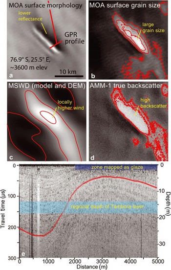
We examined the transition in satellite remote-sensing characteristics in more detail using the GPR traverse of an isolated wind-glaze region in Dronning Maud Land mapped by the Norway-US traverse in 2007 (Figs 5 and 6). The test area was first identified as an anomalous low-reflectivity feature in the MOA visible-band mosaics (Fig. 5a). The feature is ~14km x 3.5 km, with the longer dimension perpendicular to the mean wind. Both grain size and backscatter increase significantly over the feature relative to surrounding areas (Figs 5b and c). The feature lies within a band of increased MSWD, and is centered on a local MSWD maximum (Fig. 5d). Southwest of the wind-glaze feature lies a parallel pair of narrow transverse dunes, the largest being ~12km x 1.5 km. Both backscatter and surface grain size decrease significantly over the dunes. Depth to the traced reflector (Tambora horizon, 1815 CE from adjacent ice cores) decreases to 4.5 m near the center of the feature, equating to a SMB of 8.2 kgm-2 a-1 (Fig. 5e). Background regional SMB ranges from 26 to 35 kgm-2 a-1. Although accumulation increases significantly within the dune region (to a peak of 67kgm-2a-1), the extent of the locally increased accumulation is not sufficient to offset the reduced accumulation over the more extensive glaze region. Both satellite radar backscatter and surface grain size change significantly and abruptly as net SMB decreases below 20-22 kgm-2 a-1, identifying the wind-glaze region (Fig. 6). Similar shifts are noted in the satellite remote-sensing values of the other field sites, consistently near the 20kgm-2a-1 level (Fig. 7). We stablish an empirical threshold for wind-glaze feature mapping based on a line in grain-size-backscatter space that best segregates regions with a SMB below 20 kgm-2 a-1 from their surroundings:
Fig. 5. Remote-sensing data and field GPR profile across a wind-glaze site in central Dronning Maud Land. (a) MODIS Mosaic of Antarctica image of the glaze site. MOA surface reflectance is relative (arbitrary units). (b) Springtime surface snow grain size from MODIS bands 1 and 2. Contour values for surface optical snow grain size are 140, 120 and 100 µm, background is 85-95 mm. (c) MSWD for the region has contour values of 0.002 and 0.004. (d) Radar backscatter from AMM-1 compilation. Contour values for radar backscatter are -5 and -7.5 dB; background is generally-9 to -11 dB. (e) GPR profile from traverse across the site. Red trace in radar profile is the depth to the Tambora-level (1815 CE) isochrone; cyan bar shows range of accumulation from other GPR data in the region, and purple bar shows extent of wind-glaze surface as mapped by the final algorithm. The radar profile is not corrected for surface slope. In this area, the region of <20 kg m-2 SMB is approximately bounded by the areas of >-6.5 dB backscatter and >120 mm grain size. Nearly all of the mapped glaze extent lies within the 0.003 MSWD level.

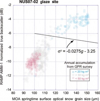
Fig. 6. Mean springtime surface optical grain size (2003 and 2008 austral springs) from MODIS data versus RADARSAT C-band backscatter along a GPR traverse across a wind-glaze region in Dronning Maud Land. Ranges of SMB derived from the GPR traverse are shown as different symbol colors. The main mapping criteria for determining criteria for determining wind-glaze regions derived from all field datasets are shown.

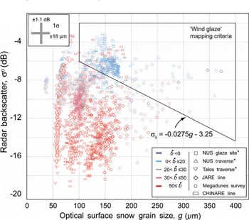
Fig. 7. MODIS-derived springtime surface optical snow grain size versus RAMP AMM-1 radar backscatter for the field measurement sites. The selection line used for estimating regional wind-glaze extent is shown, as are other thresholds used to eliminate non-glaze areas from the calculation (at grain sizes <100 and >400 µm, and backscatter >-2 dB). Symbol color indicates SMB range; symbol type indicates SMB dataset. Asterisks next to the field SMB dataset indicate these data were subset, showing only every fifth data point for clarity.

where σ0is true radar backscatter (normalized to 27° incidence angle) and g is springtime optical surface grain size (mm). Errors in the coefficient and constant in the linear equation are controlled by the measurement errors in the satellite data. As noted for Figure 6, transitions between glaze and non-glaze physical characteristics and remote- sensing values are generally abrupt.
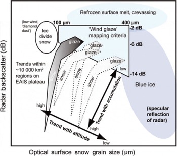
The remote-sensing characteristics of other areas of the East Antarctic plateau above the 1500 m elevation threshold led us to establish other approximate criteria for wind-glaze mapping (Fig. 8). Based on data from the highest-altitude portions of the Norway-US traverse and JARE stake line, we determined that the highest ice divide and summit areas have very low surface accumulation, approaching 20kgm-2a-1, and show increased radar backscatter but very low surface grain size. We attribute this to a high proportion of 'diamond dust' accumulation, and a combination of very low wind speed and significant subsurface recrystallization due to slow burial. Known blue-ice areas in the study area show a trend toward reduced backscatter and very high surface optical grain size. Past studies using band-ratio approaches to map blue-ice extent established a value of 400 mm as a useful edge of blue-ice extent (Reference Brown and ScambosBrown and Scambos, 2004);and low backscatter of blue-ice regions is attributed to specular reflection of the radar beam away from the satellite (e.g. Reference Fahnestock, Bindschadler, Kwok and JezekFahnestock and others, 1993). Very high-backscatter areas (σ0>-2dB) above 1500 m are rare but may be associated with crevassing or refrozen surface melt layers. To eliminate these non-wind-glaze areas from our mapping we established additional criteria (Figs 7 and 8):

Fig. 8. Diagram of surface optical grain size versus radar backscatter showing characteristics and trends of various surface types for the East Antarctic plateau.
Overall, these threshold characteristics seem reasonably robust across the high-elevation portions of the EAIS, but there are regional variations that suggest further climate- related variations in accumulation and wind-glaze formation (Fig. 8). Regionally (in areas of a few thousand square kilometers) a distinctive nonlinear relationship is seen between snow grain size and radar backscatter. Windward slopes and extensive low-slope areas consistently show the lowest local backscatter and smallest surface grain size, which grades approximately linearly until reaching the (empirical) wind-glaze threshold of 20kgm-2a-1. Across that threshold, with further decrease in accumulation, surface optical snow grain size increases significantly. These trends are qualitatively consistent but vary with regional altitude and regional mean accumulation (see Fig. 8), with locally higher accumulation generally leading to finer grain size and significantly higher radar backscatter for the trend. This relationship shows promise for future mapping of accumulation rate directly from high-resolution satellite remote-sensing data.
Errors in glaze extent mapping
Errors of omission and commission occur in the mapping, as is apparent in Figure 7. We estimate errors by the number of radar measurement points or stake sites that were incorrectly mapped (based on the field data) by our empirical linear relationship and the additional bounding thresholds. For sites with accumulation measurements averaged over centuries (e.g. site shown in Figs 5 and 6, and other data from the Norway-US traverse), errors in the glaze mapping are low: 0.7% (13 out of 1799 points) overall, 1.6% mapped incorrectly as glaze (commission;6 of 368 points) and 0.5% mapped incorrectly as non-glaze (omission;7 of 1432). The classification errors in both cases cluster near the threshold of 20kgm-2a-1, reducing their impact on estimates of reduced SMB from glaze extent. For the Talos Dome traverse data, which had significantly higher accumulation than 20kgm-2a-1 at all points, there were no classification errors. For the other field measurement sites, classification errors are larger due to poorer in situ determination of accumulation and edge effects. For the JARE line (with net accumulation based on 14 years of snow stake measurements), classification errors are 26% commission (10 of 37 points) and 4.3% omission (18 of 416 points), overall 6%. At the megadune site, errors were 18% commission (28 of 155 points) and 15% omission (26 of 175 points), overall 16%; however, for this surface type, dune migration leads to thin surface layers of new accumulation underlain by former glaze surfaces, resulting in different sources for the surface grain size and backscatter properties at the dune boundaries. As discussed above, lower regional grain size along much of the CHINARE traverse may have partially affected the assessment of glaze extent there. With the relationship developed using the overall collection of field data, the CHINARE dataset has 9% errors of commission (40 of 448 points mis-mapped as glaze) overall and 45% errors of omission (36 of 80 persistently low-accumulation sites not mapped as glaze). However, if we adjust the surface grain size by 50mm (i.e. essentially eliminating the regional pattern of lower 2008 grain size) we reduce the error of omission to 34% (27 of 80 points). We adopt an estimated error of ±15% for the glaze-mapped area as a combined value for omission and commission errors.
Results
We now apply the equation and other criteria determined above to the entire East Antarctic plateau to estimate glaze extent using the 125 m gridded remotely sensed datasets. Total glaze area extent for the EAIS above 1500 m elevation is 950 ± 143 x 103 km2 using the described thresholds. This is 11.2 ± 1.7% of the total surface area at that altitude or higher (Fig. 9 ; Table 1). Glaze extent above 2500 m is 552 ± 83 x 103 km2, or 10.0 ± 1.5% of the surface.

Fig. 9. Distribution of glaze regions (cyan) in East Antarctica, showing the major drainage basins for the ice sheet. The 1500 and 2500m elevation contours are shown in dark blue. Drainage basins are labeled with abbreviations of local major features or research bases. Clockwise from center left: By-Bd, Byrd–Beardmore region; Sf-Fo, Support Force–Foundation region; Re-Sl, Recovery–Slessor region; Lz, Lazarev Ice Shelf region; WE, West Enderby region; Mw, Mawson Coast region; Mk, MacKenzie Bay region; La, Lambert region; Gr, Grove Mountains region; Me-Ck, Mertz–Cook region; Dv, David region. See Table 1.
Table 1. Surface area and mass input of East Antarctica and several EAIS catchment basins, and amount of total mass input and SMB attributed to wind-glaze areas
Glaze is widespread across many of the major catchment basins of the EAIS. Catchments with the highest total glaze area are the Byrd-Beardmore basin, Recovery-Slessor region and Lambert Glacier. Catchments with the highest percentage of glaze area are Mawson Coast, Mertz-Cook region and the Lambert Glacier catchment. Extensive contiguous regions of glaze occur, notably in the northern Byrd-Beardmore catchment, Recovery-Slessor catchment, western Lambert basin, the Mawson Coast and upper Mertz-Cook area. In several regions, the extensive glaze areas are truncated by our 1500 m elevation threshold. Additional wind-glaze areas exist for some distance below this level, mainly in confluence areas of katabatic wind (e.g. David basin; Mertz–Cook area (Reference Frezzotti, Gandolfi, La Marca and UrbiniFrezzotti and others, 2002a; Reference Scarchilli, Frezzotti, Grigioni, De Silvestri, Agnoletto and DolciScarchilli and others 2010); however, our selection criteria would have included increasing errors due to short-term surface glazing, crevassing and melt-layer effects. Surface glazing was noted at lower elevations on the Talos Dome traverse (for example), but accumulation rates along the traverse remained high.
Given the widespread glaze extent, and the evidence that they represent persistent near-zero accumulation surfaces, we examine the amount of accumulation attributed to glaze areas using three recent estimates of Antarctic SMB (Figs 9 and 10; Table 1; Reference Arthern, Winebrenner and VaughanArthern and others, 2006;Reference Monaghan, Bromwich and WangMonaghan and others, 2006;Reference Lenaerts, Van den Broeke, Van de Berg, Van Meijgaard and Kuipers MunnekeLenaerts and others, 2012). For glaze areas above 1500 m, a total of 46.3-82.4Gta-1 of input mass is attributed to glaze areas, with mean attributed SMB rates of 49-87 kg m-2 a-1. For regions above 2500 m, input mass values of 17.2-34.4Gta-1 are attributed, with mean SMB of 31-62 kg m-2 a-1. Even with substantial extents of adjacent high-accumulation regions, it is unlikely that these overestimates can be rebalanced to the mean modeled accumulation for glaze regions. Moreover, the large contiguous regions of glaze mapped in the Byrd-Beardmore, Lambert, David, Mawson and Mertz-Cook have no high-accumulation regions of sufficient extent to offset the near-zero SMB of the mapped glaze areas.

Fig. 10. Mapped wind-glaze extent (grey) plotted over three color-coded recent net SMB maps of East Antarctica: (a) Reference Lenaerts, Van den Broeke, Van de Berg, Van Meijgaard and Kuipers MunnekeLenaerts and others (2012); (b) Reference Arthern, Winebrenner and VaughanArthern and others (2006); (c) Reference Monaghan, Bromwich and WangMonaghan and others (2006). Drainage regions as in Figure 9; the 1500 and 2500m elevation contour from Reference Bamber, Gomez-Dans and GriggsBamber and others (2009) is shown as a red line.
Figure 11 examines the distribution of wind glaze as histograms of gridcells mapped as glaze relative to MSWD model values and DEM elevation (RACMO2/ANT; Reference Bamber, Gomez-Dans and GriggsBamber and others, 2009; Reference Lenaerts, Van den Broeke, Van de Berg, Van Meijgaard and Kuipers MunnekeLenaerts and others, 2012). Glaze extent peaks at values of 0.00075-0.0016 MSWD (unitless, or mm-1) and elevations of 2685-2900m. These values compare well with MSWD for megadune regions (average slope of a megadune field, including glaze and accumulating dune areas, generally 0.0010-0.0016; Reference Frezzotti, Gandolfi, La Marca and UrbiniFrezzotti and others, 2002a), but our mean value is significantly lower than the values these studies determine for individual glaze surfaces (>0.004). Our MSWD mapping is based on a satellite altimetry DEM, which has a true resolution scale of 3-8 km (Reference Bamber, Gomez-Dans and GriggsBamber and others, 2009). This is much coarser than the remote-sensing-based parameters, and is also a larger scale than true surface undulations. In other words, the mean slope measurements and derived MSWD are somewhat too coarse to capture the glaze areas discretely. Mean elevation for all cells mapped as glaze is 2585 m. Wind-glaze area drops off abruptly above 3400 m, approaching the elevation of the ice divides in the EAIS.

Fig. 11. Histograms of number of cells (125m nominal scale) mapped as wind glaze as a function of (a) MSWD and (b) elevation (from Reference Bamber, Gomez-Dans and GriggsBamber and others, 2009; Reference Lenaerts, Van den Broeke, Van de Berg, Van Meijgaard and Kuipers MunnekeLenaerts and others, 2012).
The Reference Lenaerts, Van den Broeke, Van de Berg, Van Meijgaard and Kuipers MunnekeLenaerts and others (2012) SMB estimates from the RACMO2/ANT climate model are consistently lower than the other two SMB estimates, and for two of the basins (Byrd-Beardmore and David) this estimate attributes a net mass balance of <20 kg m-2 a-1 for glaze areas, as our study indicates (Table 1). This model modifies input snowfall with enhanced sublimation and redistribution from drifting snow, and benefits from a higher-resolution surface wind field model (which is driven primarily by inversion gravity-driven forcing in the upper EAIS; Reference Van, Broeke, Van Lipzig and Van MeijgaardVan den Broeke and others, 2002). However, all three models likely attribute too great a SMB value to some of the basin regions, specifically those close to the coast: Mawson Coast, MacKenzie Bay, Mertz-Cook, and Lazarev Ice Shelf catchment regions. The implication is that net SMB in all current models of the EAIS is too high by an amount large enough to impact estimates of mass balance for the ice sheet, in these regions in particular. Specifically, mass-balance estimates based on mass budget methods should account for overestimated accumulation in the basins with the highest proportions of glaze and highest SMB attributed to glaze shown in Table 1. Elevation-change- based estimates (dH/dt, or volumetric measures of ice-sheet mass balance) or gravity-based estimates (from the Gravity Recovery and Climate Experiment (GRACE) satellite) will be relatively unaffected.
Discussion
The mapping we present, and the physical characteristics used to identify wind-glaze regions, essentially describe a new surface facies type for ice sheets, as distinctive as those in Reference BensonBenson's (1960) landmark study. Recent studies, and studies in preparation as of this writing, have identified many extensive regions of wind glaze in the East Antarctic plateau region, and have variously attributed them to long-term 'hiatuses' in accumulation or buried ablation areas formed in past glacial epochs (Reference Siegert, Hindmarsh and HamiltonSiegert and others, 2003;Reference Wen, Jezek, Monaghan, Sun, Ren and HuybrechtsWen and others, 2006; Reference Arcone, Jacobel and HamiltonArcone and others, 2012).
Reference Siegert, Hindmarsh and HamiltonSiegert and others (2003) identify buried unconformable reflections in GPR data in the catchment regions of Byrd and Nimrod Glaciers. They note that if the missing surface layers were removed by ablation, then a large region of blue ice would be exposed, and that this may be shallowly buried beneath new accumulation. The regions identified by Reference Siegert, Hindmarsh and HamiltonSiegert and others (2003) lie very close to areas mapped as extensive surface glaze here, and we infer from the new evidence we present that these areas are sites of very longterm accumulation hiatus due to the wind-glaze processes. Reference Wen, Jezek, Monaghan, Sun, Ren and HuybrechtsWen and others (2006) examined accumulation variability in the region of the ANARE (Australian National Antarctic Research Expeditions) Lambert Glacier basin traverse. Their analysis of stake accumulations over the period 1990-94 and 1998 shows high local (2 km scale) variability, with many near-zero net snow measurements, but few negative SMB sites. Further, their study identifies broad areas in the Lambert catchment system where their interpolated estimate of mean SMB falls significantly below that of the two models they use in comparison (Antarctic Mesoscale Prediction System (AMPS) and Polar fifth generation Mesoscale Model (MM5);Reference Powers, Monaghan, Cayette, Bromwich, Kuo and ManningPowers and others, 2003;Reference Bromwich, Guo, Bai and ChenBromwich and others, 2004). The regions of low accumulation closely approximate our mapped areas of extensive wind glaze.
Similarly, Reference Arcone, Jacobel and HamiltonArcone and others (2012) identify large expanses of zero-accumulation surface interspersed with local high-accumulation regions. They argue for intensified accumulation in these isolated (glaze-surrounded) regions, well above any measured accumulation rates in the literature for the area of their study (Byrd Glacier catchment), and several-fold above that required for balance of Byrd Glacier (e.g. Reference StearnsStearns, 2007). However, the model approach taken by Reference Arcone, Jacobel and HamiltonArcone and others (2012) assumes that regional accumulation values from models were accurate (specifically those from Reference Vaughan, Bamber, Giovinetto, Russell and CooperVaughan and others, 1999;Reference Arthern, Winebrenner and VaughanArthern and others, 2006;Reference Van de Berg, Van den Broeke, Reijmer and Van MeijgaardVan de Berg and others, 2006), and then concludes that they underestimate regional accumulation. Reference StearnsStearns (2011) uses the pre-Reference Lenaerts, Van den Broeke, Van de Berg, Van Meijgaard and Kuipers MunnekeLenaerts and others (2012) accumulation values for four major EAIS outlet glaciers and concludes that all may be impacted by overestimates of SMB in their catchments. The SMB values of Reference Lenaerts, Van den Broeke, Van de Berg, Van Meijgaard and Kuipers MunnekeLenaerts and others (2012) greatly reduce the positive imbalance for these outlets.
The present assessment of accumulation in extensive glaze areas suggests that ice balance velocities should also be reduced in these areas. A comparison of actual velocity (measured by interferometric SAR for regional comparisons, or a GPS for point measurements) with current models of balance velocity would confirm whether glaze-prevalent regions in fact represent accumulation deficits, or are balanced by adjacent higher-accumulation regions. Far less mass input to the system (our conclusion), and the steady- state assumption (no ongoing surface elevation change) in surface balance velocity calculations leads to a reduction in the ice flow velocity needed to distribute surface infall to the margins in the ice-sheet system. However, the comparison requires a significant amount of glaze area upflow of the measurement site. The lower-elevation regions of megadune areas, or the zones of contiguous glaze shown in Figure 9, are the most likely locations where measured velocities should be considerably lower than those estimated from earlier SMB models (especially pre-Lenaertz and others, 2012).
Why should regions of wind glaze (and their adjacent accumulation highs) represent a net loss of snow mass? Many studies to date have assumed that wind redistribution of snow was a mass-conservative process, and that mass lost from windswept regions was deposited in adjacent areas of accumulation. All of the field datasets we present (Figs 2, 4 and 5, and data from the megadune field sites; Scambos and others 2006; Reference Courville, Albert, Fahnestock, Cathles and ShumanCourville and others, 2007;Frezzotti and others 2007; Reference Scarchilli, Frezzotti, Grigioni, De Silvestri, Agnoletto and DolciScarchilli and others, 2010) show that in fact adjacent areas of above-regional-mean accumulation are smaller in extent and insufficient to compensate for the surface loss. We attribute the net loss to adiabatic heating and drying of the inversion air layer, and the local increase in wind speed over glaze regions. The downflowing air sublimates entrained blowing snow. At the lower-elevation edge (or down-airflow edge of a steeper MSWD region), part of the entrained mass of blowing snow has been converted to water vapor, and is carried on with the katabatic flow even though the airflow slows and allows the remaining snow to accumulate in the glaze-adjacent dune. This was partially discussed by Reference Neumann, Waddington, Steig and GrootesNeumann and others (2005) and is mentioned qualitatively in numerous studies. Modeling of this process for a glaze region, and extending the study to regional scales where glaze is prevalent, is a suitable avenue for future work.
Conclusions
Wind-glaze areas can be mapped based on their remote-sensing characteristics, which are derived from unique physical characteristics due to persistent low accumulation in windswept parts of ice sheets, primarily the middle elevations of the EAIS. They are widespread, and cover extensive contiguous areas in the EAIS interior. In regions nearer the coast, all current SMB models tend to overestimate the surface mass input to glaze regions, and many recent SMB models overestimate wind-glaze mass balance in all areas. Glazed area with SMB <20 kgm-2 a-1 represents ~11% of the area above 1500 m and represents generally the lower limit (hiatus in accumulation) of SMB of the EAIS, excluding blue-ice areas that represent ~1% of the surface (and are generally limited to coastal areas and regions adjacent to nunataks). Our analysis suggests that all current SMB models for the EAIS overestimate mass input to the ice sheet by 46-82 Gta-1. Moreover, extensive wind erosion areas are present below 1500 m, where snow precipitation is on average higher. These could not be accounted for in this paper due to the limitations of our remote-sensing analysis. Therefore, our evaluation of EAIS SMB decrease due to the extent of wind-glazed surfaces must be taken as a lower limit of the overestimation.
Inclusion of drifting-snow physics (entrained-snow sublimation) in regional climate models improves the representation of low-SMB and -ablation areas. Running these models at higher resolution (5 km or less) should resolve wind-glaze areas discretely and could potentially quantify the processes responsible for their formation and persistence.
Most important, however, are the implications for continental mass balance. Our study indicates that glaze areas are extensive enough to have a significant impact on current estimates of SMB, and therefore overall mass balance using the mass budget method (MBM; e.g. Reference RignotRignot and others, 2008). The scale of the overestimate is equal to the total error reported for East Antarctica (±61 Gta-1; Reference RignotRignot and others, 2008) and a large fraction of the currently reported error bars for Antarctic-wide mass balance (±150Gta-1; Rignot and others, 2011). Moreover, the error represented by the SMB overestimate over wind-glaze regions moves the MBM results in the direction of GRACE-based results for Antarctica as a whole and for the East Antarctic ice sheet (Reference VelicognaVelicogna, 2009; Rignot and others, 2011). Elevation- change-based estimates (dH/dt, or volumetric measures of ice-sheet mass balance) or gravity-based estimates (from the GRACE satellite) will be relatively unaffected by these results, if performed at a decadal averaging scale.
Acknowledgements
This work was supported by NASA grants NNG04GM10G and NNX10AL42G, and US National Science Foundation grant 0PP-0538495 (T.S., T.H., J.B., T.N. and M.A.). We acknowledge the ice2sea project, funded by the European Commission's 7th Framework Programme through grant No. 226375, manuscript No. ice2sea072. We thank the staff of Raytheon Polar Services, the Norsk Polarinstitutt, the field team of the Norwegian-US International Polar Year (IPY) Scientific Traverse, and the 109th Air National Guard and Ken Borek Air for their logistical help during Antarctic fieldwork.