


1. INTRODUCTION
Rapid mass loss from calving glaciers is influencing the large-scale mass loss of ice sheets, icefields and glaciers (Gardner and others, Reference Gardner2013). Calving, or iceberg detachment from glacier termini, is known to be the most significant processes for mass loss from calving glaciers in Patagonia (Rignot and others, Reference Rignot, Rivera and Casassa2003; Schaefer and others, Reference Schaefer, Machguth, Falvey, Casassa and Rignot2015), Alaska (Arendt and others, Reference Arendt, Echelmeyer, Harrison, Lingle and Valentine2002; Larsen and others, Reference Larsen2015; Truffer and Motyka, Reference Truffer and Motyka2016), half the mass loss from the Greenland ice sheet (van den Broeke and others, Reference van den Broeke2009; Enderlin and others, Reference Enderlin2014) and nearly 45% of the mass loss from the Antarctic ice sheet (Rignot and others, Reference Rignot, Jacobs, Mouginot and Scheuchl2013). Particularly in the Patagonia icefields, which form the largest temperate glacier system in the Southern Hemisphere, ice mass is being lost at one of the fastest rates in the world (Jacob and others, Reference Jacob, Wahr, Pfeffer and Swenson2012; Gardner and others, Reference Gardner2013). Of 69 major outlet glaciers in the region, more than 90% of ice fronts end in lakes and the ocean (Warren and Aniya, Reference Warren and Aniya1999). The front positions of these calving glaciers have been retreating over the last few decades (Aniya and others, Reference Aniya, Sato, Naruse, Skvarca and Casassa1997; Rignot and others, Reference Rignot, Rivera and Casassa2003; Lopez and others, Reference Lopez2010) as a result of increasing ice discharge through calving (Sakakibara and Sugiyama, Reference Sakakibara and Sugiyama2014; Schaefer and others, Reference Schaefer, Machguth, Falvey, Casassa and Rignot2015), causing the rapid mass loss of the ice fields (Willis and others, Reference Willis, Melkonian, Pritchard and Rivera2012).
Seismic signals have been used to monitor calving activity in Greenland (Amundson and others, Reference Amundson2008, Reference Amundson2010; Tsai and others, Reference Tsai, Rice and Fahnestock2008; Nettles and Ekström, Reference Nettles and Ekström2010; Walter and others, Reference Walter, Olivieri and Clinton2013), Alaska (O'Neel and others, Reference O'Neel, Marshall, McNamara and Pfeffer2007; Bartholomaus and others, Reference Bartholomaus, Larsen, O'Neel and West2012, Reference Bartholomaus2015), Antarctica (MacAyeal and others, Reference MacAyeal, Okal, Aster and Bassis2009; Chen and others, Reference Chen, Shearer, Walter and Fricker2011) and Svalbard (Köhler and others, Reference Köhler, Chapuis, Nuth, Kohler and Weidle2012, Reference Köhler, Nuth, Schweitzer, Weidle and Gibbons2015, Reference Köhler2016). These studies revealed that calving, which does not involve capsizing, generates a distinctive frequency of seismic signals between 1 and 3 Hz (O'Neel and others, Reference O'Neel, Marshall, McNamara and Pfeffer2007; Podolskiy and Walter, Reference Podolskiy and Walter2016). Moreover, Bartholomaus and others (Reference Bartholomaus2015) revealed that seismic signals were useful, not only to detect glacier calving, but also to locate calving events, characterize the calving style and estimate calving flux. Similar to these seismic signal studies, additional work endeavored to use acoustic signals to study calving (Pettit, Reference Pettit2012; Pettit and others, Reference Pettit, Nystuen and O'Neel2012, Reference Pettit2015; Deane and others, Reference Deane, Glowacki, Tegowski, Moskalik and Blondel2014; Glowacki and others, Reference Glowacki2015). These studies revealed that high-frequency acoustic signals (up to several tens of kilohertz) could be used to detect individual calving events (Glowacki and others, Reference Glowacki2015).
When icebergs break off into the water, surface-water waves arise over the ocean or a lake in front of calving glaciers. Several studies have been used to study surface waves to understand calving processes by in situ observations (Haresign, Reference Haresign2004; Iizuka and others, Reference Iizuka, Kobayashi and Naruse2004; Marchenko and others, Reference Marchenko, Morozov and Muzylev2012; Lüthi and Vieli, Reference Lüthi and Vieli2016; Vaňková and Holland, Reference Vaňková and Holland2016) and numerical modeling (Massel and Przyborska, Reference Massel and Przyborska2013). For example, Iizuka and others (Reference Iizuka, Kobayashi and Naruse2004) observed surface waves in front of Glaciar Perito Moreno (GPM), a lake-terminating glacier in the Southern Patagonia Icefield (SPI). They collected 12 d of surface-wave observations with sampling rates of 5 or 15 s measuring 68 events generated by calving. The maximum amplitude was 0.48 m, and water-level oscillations lasted for ~50 min. According to seismic and acoustic signal studies, signal frequency contains important information about calving size and style (e.g., Bartholomaus and others, Reference Bartholomaus2015; Glowacki and others, Reference Glowacki2015). However, with low sampling rates of 5–15 s, information can be undersampled and lost. Vaňková and Holland (Reference Vaňková and Holland2016) performed year-round surface-wave observation at five sites by using bottom pressure meters attached to a mooring in Sermilik Fjord, East Greenland. However, because the closest sensor was located 30 km away from Helheim Glacier, they observed only 16 events generated by calving. Surface waves attenuate with distance, and high-frequency waves decay faster than low-frequency waves (Lamb, Reference Lamb1932). Therefore, it is important to observe surface waves in the vicinity of a glacier front. By using numerical modeling, Massel and Przyborska (Reference Massel and Przyborska2013) studied idealized wave propagation from an object falling into water for four different scenarios and obtained different wave patterns for various source mechanisms. These studies implied that observations of surface waves are useful not only for monitoring calving activity, but also for characterizing calving style or size. However, to our knowledge, there is no such detailed study with relatively long-term surface-wave observations near a glacier front.
In terms of calving mechanisms, calving can be classified into four different styles (Benn and others, Reference Benn, Warren and Mottram2007). The first style is subaerial calving of a piece of ice falling from an ice cliff. This style involves the propagation of a fracture due to ice flow velocity gradient (e.g., Meier and Post, Reference Meier and Post1987) and/or undercutting by high subaqueous melting (e.g., Motyka and others, Reference Motyka, Hunter, Echelmeyer and Connor2003; Bartholomaus and others, Reference Bartholomaus, Larsen, O'Neel and West2012). Secondly, when a glacier flows into a deep fjord, the ice front is close to flotation. The ice velocity gradient and high buoyancy may enhance crevasses from the glacier bottom to the surface and generate full-ice-thickness tabular icebergs in grounded glaciers that frequently capsize after detaching (Howat and others, Reference Howat, Joughin and Scambos2007; Amundson and others, Reference Amundson2010; Bassis and Jacobs, Reference Bassis and Jacobs2013; James and others, Reference James, Murray, Selmes, Scharrer and O'Leary2014). In addition to this, tabular icebergs sporadically detach from the freely floating ice tongues and ice shelves when a glacier flows into cold water (Lazzara and others, Reference Lazzara, Jezek, Scambos, MacAyeal and Van der Veen1999; Warren and others, Reference Warren, Benn, Winchester and Harrison2001; Boyce and others, Reference Boyce, Motyka and Truffer2007; Bassis and others, Reference Bassis, Fricker, Coleman and Minster2008; Trüssel and others, Reference Trüssel, Motyka, Truffer and Larsen2013; Truffer and Motyka, Reference Truffer and Motyka2016). Thirdly, similar to subaqueous melting, thermal notch formation at the waterline has also been suspected as a driving mechanism of subaerial calving (e.g., Kirkbride and Warren, Reference Kirkbride and Warren1997; Röhl, Reference Röhl2006; Minowa and others, Reference Minowa, Sugiyama, Sakakibara and Skvarca2017). Finally, for the fourth calving style, ice detaches not only from the subaerial part of a calving front, and sometimes icebergs float up from underwater (e.g., Hunter and Powell, Reference Hunter and Powell1998; Truffer and Motyka, Reference Truffer and Motyka2016). These icebergs usually contain debris. However, in general, neither a question about how common each calving style is, nor a question which calving styles can be associated with surface waves are well addressed.
In this study, we measured surface waves generated by calving events at GPM, a lake-terminating glacier, in the SPI at 300–1800 m distance from the calving front. First, we confirmed with time-lapse photography analysis that glacier calving generates surface waves that are distinctive from other local sources such as wind or tourist boats. Next, we developed a detector to count the occurrence rate based on a prescribed threshold for wave height, as well as a distance estimator based on dispersion analysis. Corresponding calving styles were classified by using time-lapse images. These surface waves and corresponding calving styles enable us to explore the properties of surface waves generated by glacier calving for conditions of a lake-terminating glacier.
2. STUDY SITE
GPM (50.5°S, 73.2°W) stretches over a length of 30 km from Cerro Pietrobelli (2950 m a.s.l.) to Lago Argentino (177.5 m a.s.l.). The glacier covers an area of 259 km2 (De Angelis, Reference De Angelis2014), and calves into two lakes, Brazo Rico and Canal de los Témpanos, which are a part of Lago Argentino (Fig. 1). The lower part of the glacier is heavily crevassed due to a divergence of the flow field, and icebergs frequently break off from the calving front (Fig. 1b). The height of the ice cliff above the lake surface is between 55 and 75 m (Naruse and others, Reference Naruse, Fukami and Aniya1992). Water depth near the calving front in Brazo Rico is shallower than 70 m, and deepens to ~120 m about 500 m from the ice front (Fig. 1b) (Sugiyama and others, Reference Sugiyama2016). According to previous observations on the glacier surface elevation and bathymetry at GPM, the glacier is well above the flotation level (Naruse and others, Reference Naruse, Fukami and Aniya1992; Sugiyama and others, Reference Sugiyama2016). Therefore, we would expect the ice front to be grounded.

Fig. 1. (a) A map showing the study site. (b) Satellite image of Glaciar Perito Moreno with instrument locations. The background image was taken by ALOS/PRISM on 29 March 2008. Lake bathymetry in front of Glaciar Perito Moreno with contour intervals of 10 m. Circles indicate distances every 250 m from the water pressure sensor (blue square). (c) Photograph of the pressure measurement site.
In Brazo Rico, there are two possibilities for non-calving events to disturb surface-wave observation. Since GPM is listed as a World Heritage Site in Argentina, a large number of tourist boats visit the glacier frequently during the day. Boats cruise along the glacier front and some of the tourists come ashore to walk to the glacier from the harbor (Fig. 1b). Also, as it is aptly referred to as the Land of Tempest (Shipton, Reference Shipton1963), Patagonia is characterized by consistently strong westerly winds and the wind speed is enhanced particularly in summer (Stuefer, Reference Stuefer1999; Lenaerts and others, Reference Lenaerts2014), leading to the generation of surface waves.
3. METHODS AND DATA
3.1. Time-lapse photography
To observe glacier calving, we took photographs of the calving front every 1 min with time-lapse cameras (GardenWatchCam, Brinno Co., Taipei 1280 × 1024 pixels, with 5.01 mm focal length, and corresponding ice cliff height from ~100 to 150 pixels). The photographs were utilized to distinguish calving-generated surface waves from those due to other sources. Cameras were installed at four different positions during the field observations (Fig. 1): camera 1 was operated from December 2013 to January 2014 and in October 2014, camera 2 from December 2013 to January 2014, camera 3 from February to March 2016 and camera 4 in October 2014. No images were recorded at nighttime. Typically, daylight hours were 19% longer in December (16 h) compared with October (13 h) during the observations.
We categorized the calving events that were observed into four groups (Fig. 2): Topple – an ice tower toppling into the lake; Drop – an ice block dropping into the water; Serac – serac slipping down to the lake; and Subaqueous – iceberg floating up to the lake surface. These were the most common calving styles in GPM, and 420 calving events in total were classified over the three periods (Table 1). Although the shooting interval was relatively low, sequences of the time-lapse camera images provided sufficient information to distinguish the styles. We distinguished Topple from Drop by observing crevasse widening. Topple was observed after crevasse opening for several minutes, while Drop occurred without any precursors (Fig. 2). Subaqueous calving was distinguished from other subaerial calving by noting a lack of frontal changes and sediment inclusion in icebergs. When subaqueous caving occurred, a relatively large single iceberg appears without any geometrical change above the water surface. We sometimes observed debris-rich icebergs, which indicated their basal origin. Location of each calving event was mapped onto a Landsat-8 Operational Land Imager (OLI) band 8 image (15 m resolution) based on distinctive ice features (ice front geometry, large crevasses, ice tower), which were recognizable on the time-lapse and satellite images (Fig. 3). The Landsat images were taken on 10 December 2013, 3 October 2014 and 22 March 2016.
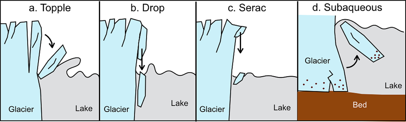
Fig. 2. Illustration of the most common calving styles at GPM.

Fig. 3. Satellite images showing the location of calving events obtained by comparing time-lapse and satellite images in (a) period 1, (b) period 2 and (c) period 3 (marker size is proportional to the number of events). Blue squares and green diamonds indicate the location of the water pressure sensor and time-lapse cameras, respectively. Contours indicate water depth with intervals of 20 m. (d)–(f) Histograms of source-to-sensor distance determined from (a)–(c). Vertical dashed red lines indicate the locations of subaqueous calving. (g)–(j) Examples of the time-lapse camera images.
Table 1. Occurrence and fraction (% in the parentheses) of four different calving styles for periods 1, 2 and 3

3.2. Measurement of surface waves
We observed lake surface waves by operating a water pressure sensor (HOBO U20, Onset Co.) in the lake. The sensor was installed at the coast of Brazo Rico ~50 cm below the water surface by fixing the sensor on a 2 m aluminum pipe, fixing the pipe securely with boulders as shown in Figure 1c. The water depth below the sensor was ~10 m, meaning that the measurements were done not in the surf zone, which could complicate the analysis (e.g., Horikawa and Kuo, Reference Horikawa and Kuo1966). The distance from the sensor to the ice front ranged from 300 to 1800 m (Fig. 1b). We operated the water pressure sensor in three periods: period 1: 15 December 2013–4 January 2014 (19.6 d), period 2: 6–20 October 2014 (13.6 d) and period 3: 27 February–4 March 2016 (5.4 d). The accuracy of the sensor was equivalent to a water level of ±5 mm with a resolution of 1.4 mm. Water pressure was recorded every 2 s (0.5 Hz). The corresponding highest observable Nyquist frequency, i.e., half of the sampling rate, was 0.25 Hz. The water pressure P w was converted to water level H w by correcting for atmospheric pressure variations using the following equation:
 $$H_{\rm w} = (P_{\rm w} - P_{\rm a})/\rho _{\rm w}g,$$
where ρ w, g and P a are the density of fresh water (1000 kg m–3), gravitational acceleration (9.81 m s–2) and air pressure measured with a local automatic weather station (AWS) (Fig. 1b), respectively. After correcting for atmospheric pressure variations, we also applied a high-pass filter with a cutoff period of 1 h to obtain a detrended water-wave signal. Such high-pass filter was used in order to remove any seasonal variations in the lake level.
Gravitational water waves considered in this study were assumed to propagate in ice-free water (according to Landsat 8 satellite imagery and time-lapse photographs; Fig. 3). Surface gravity waves propagate according to the dispersion relationship between a wavenumber k and an angular frequency ω (Munk and others, Reference Munk, Miller, Snodgrass and Barber1963):
 $$\omega ^2 = gk\tanh (kh),$$
where k is the wavenumber (m–1; k = 2π/λ, where λ is a wavelength) and h is the water depth. In particular, in a case of λ < h, the surface wave is considered to be a deep-water wave. For deep-water waves, k is large enough to fulfill kh ≫ 1, and thus tanh (kh) ≈ 1. Therefore, the dispersion relation (Eqn 2) can be approximated as
 $$\omega ^2 = gk.$$
This equation leads to a phase velocity C = ω/k = g/ω and a group velocity U = ∂ω/∂k = g/(2ω) = C/2 (Munk and others, Reference Munk, Miller, Snodgrass and Barber1963; Bromirski and Duennebier, Reference Bromirski and Duennebier2002). The relationship U ∝ 1/ω implies that the arrival time of the surface wave generated by calving is linearly dependent on the wave frequency (MacAyeal and others, Reference MacAyeal, Okal, Aster and Bassis2009).
To investigate wave properties, we performed spectral analysis of observed surface waves. First, we calculated a spectrogram of the surface wave by using a Matlab function ‘spectrogram()’ with a moving window of 20 s and an overlap of 90% (these parameters were chosen empirically as optimal for temporal and frequency resolution). Second, we calculated power spectral density using the Matlab ‘fft()’ function with 512 (28) sampling points.
Surface-water waves associated with glacier calving were identified by defining a wave height threshold. We detect each calving event by identifying a signal with an amplitude >0.13 m. The 0.13 m threshold was determined by comparing surface waves and time-lapse images. The smallest calving event recorded by the time-lapse cameras, which was also recorded by the pressure sensor, had a 0.13 m maximum wave amplitude. However, at GPM, as we noted before, the source of surface waves was not always a result to glacier calving. During daytime hours, tourist boats approached the glacier many times. During the period indicated by the gray lines in Figure 5, the boats appeared in the photographs. The boats do generate waves, but they were smaller than the calving signals. Another possible local noise is the strong Patagonian wind. However, the wave height was <0.1 m even during the periods with winds higher than 14 m s–1. Therefore, neither the boat traffic nor wind was misinterpreted as calving in our analysis.
In order to investigate the performance of the detection method, numbers of events were obtained from surface waves and time-lapse imagery. With the 0.13 m threshold, we detected 1074 events in total, including 239 events detected at night. The number of daytime false-positive and false-negative detections were 42 and 45 events, respectively. Thus, the uncertainly of the method was 10%. The most of the false-positive detections arose from large calving events, which produced long-lasting surface waves with relatively high amplitude. On the other hand, false-negative detections were associated with small calving events, which produced small surface waves. These events were hard to detect due to their low signal-to-noise ratio.
Since the lake level occasionally dropped below the sensor level during our field activity in period 1, it is necessary to evaluate a negative wave amplitude clipping. This clipping is a possible cause of spectrum blurring and changes of their characteristics. To evaluate the influence of this effect, we artificially clipped well-recorded waves 0.1 m from their lowest negative amplitude and analyzed their spectra to see what difference was produced, if any. The power of a wave was decreased 16% from the original, whereas the general trend of the spectrum did not change except for the low frequency of the waves. At the lowest frequency of the clipped waves (<0.002 Hz), the power of the wave increased substantially when compared with the original wave. Therefore, negative amplitude clipping likely causes higher power at the low frequency, but only during period 1.
4. RESULTS
4.1. Time-lapse photography
A total of 420 events were identified by visual inspection on time-lapse camera images and manually localized on corresponding satellite imagery (Fig. 3). These calving events are non-uniformly distributed along the calving front. In period 1, a large number of events clustered at 700 and 1100–1300 m from the pressure sensor (Fig. 3d). This spatial distribution was similar in period 2 (Fig. 3e).
Among the 420 calving events, 57 events (14%) were categorized as Topple, 197 events (47%) were Drop and 156 events (37%) were Serac. Only ten events (2%) were Subaqueous (Table 1). This distribution of calving styles was similar between the three periods. Drop and Serac accounted for 80–90% of the calving events in the periods, and Topple accounted for ~15%. Subaqueous calving was observed in periods 1 (2%) and 3 (5%) but was never observed in period 2 (Table 1).
Figure 4 shows the number of calving events per day classified by their styles. Serac and Drop were more common than the other two styles and recorded every day during the three observation periods. Topple was also observed frequently, but not every day. We recorded only seven and three subaqueous-calving events in periods 1 and 3, respectively. In period 1, subaqueous-calving events occurred every day from 27 to 31 December 2013 and events were more frequent than in the other periods (Fig. 4a). Temporal variations in the daily event number was greater than those in the other two periods (Figs 4b, c).
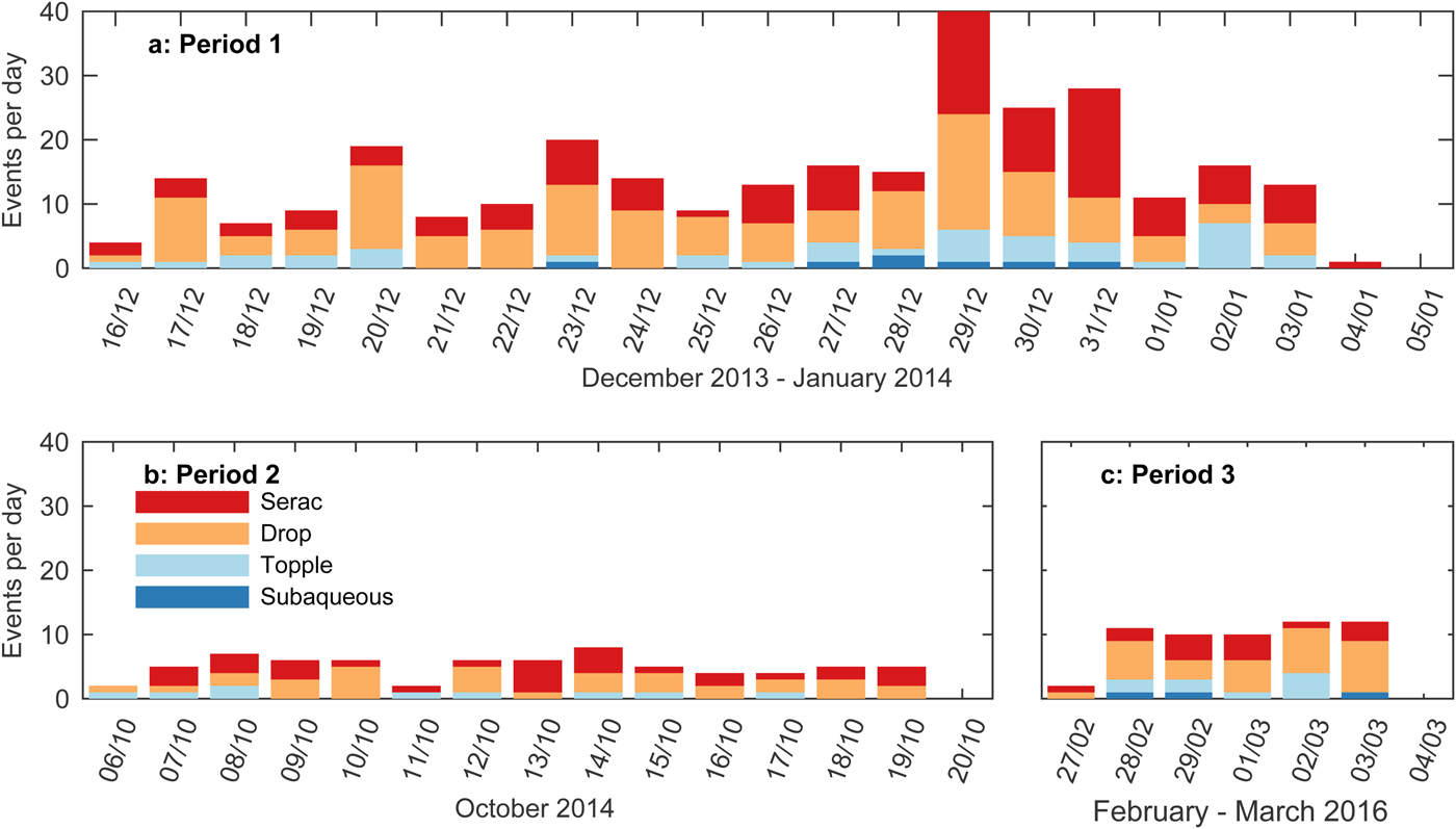
Fig. 4. Daily number of calving events classified by their style in (a) period 1, (b) period 2 and (c) period 3.
4.2. Surface waves generated by calving
Figure 5a shows an example of surface waves recorded for eight hours from 9:00 to 17:00 on 17 December 2013 in local time, during the most windy period in our observation period (Fig. 5b). When calving occurred, it generated impulse waves (Figs 5a, c). For example, we observed ten surface waves generated by calving on December 17, which were confirmed by time-lapse images (Fig. 5a). Maximum amplitude ranged from 0.13 and 0.6 m, with wave durations of ~10–30 min (Figs 5a, c). This wave height and duration are similar to those previously observed in Brazo Rico by Iizuka and others (Reference Iizuka, Kobayashi and Naruse2004). In addition to these waves caused by calving events, smaller waves were recorded and they were not associated with calving captured by the images (Fig. 5a). We assume these waves were generated by small calving, wind, boats or some other sources of noise outside the field of view.
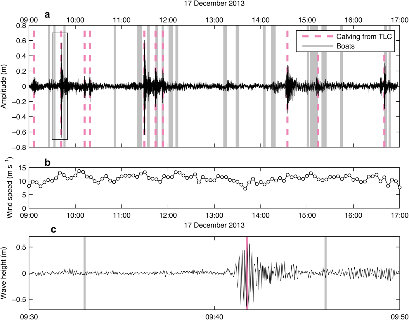
Fig. 5. (a) An example of observed surface-wave records for 8 h spanning from 9:00 to 17:00 on 17 December 2013 when the strongest westerly wind was recorded during the field campaign. Red thick dashed lines and grey lines highlight calving events observed by the time-lapse cameras and appearance of a tourist boat in the photographs, respectively. The box indicates the region enlarged in (c). (b) Wind speed recorded during the same period. (c) Enlarged surface wave between 9:30 and 9:50.
By applying the criteria of calving-generated waves described in the Methods section, we obtained 649 (33 d−1), 217 (16 d–1) and 208 events (39 d–1) during periods 1, 2 and 3, respectively (Fig. 6). In periods 1 and 3, calving occurred 2.1 and 2.4 times more frequently than in period 2. These events were non-uniformly distributed over time. For example, in period 1, the number of events increased to 6 h–1 from 27 December to 1 January and decreased towards the end of the measurements (Fig. 6a). The number of events in period 3 varied in time as well, whereas events were more uniformly distributed over time in period 2 (Fig. 6b). Despite the difference in the calving frequency, the mean maximum amplitudes were similar for all periods: 0.36 ± 0.24 m (±SD), 0.33 ± 0.22 m and 0.34 ± 0.22 m for the periods 1, 2 and 3, respectively. Figures 6 and 7 show anomaly in hourly calving rates and hourly variations in the number of events averaged over each period, respectively. Figures 6a, c suggest decrease in calving rates at night. However, there was no clear diurnal variation in the number of detected events in all the periods.

Fig. 6. Calving events detected by surface wave in (a) period 1, (b) period 2 and (c) period 3. Blue bars indicate anomaly in the event frequency relative to a 50 h moving average. Black line indicates the daily cumulative number of events. The total number of detected events and the mean calving rate are shown in each panel. Red line indicates hourly mean air temperature observed by the AWS at the glacier front.
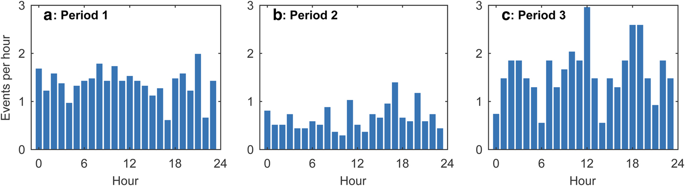
Fig. 7. Diurnal variations in the number of events detected from surface waves in (a) period 1, (b) period 2 and (c) period 3.
Figure 8 presents cumulative distribution functions of waiting time τ (min) in comparison to best-fit power-law and exponential models. The waiting time τ spanned more than one order of magnitude. The minimum τ was 5.8, 3.1 and 3.9 min in periods 1, 2 and 3, respectively. The maximum τ was 516.4, 640.5 and 323 min in periods 1, 2 and 3 with a mean τ of 43.6, 90.7 and 37.7 min, respectively. In general, the exponential distribution reproduced better the observed data than the power-law model (Fig. 8).
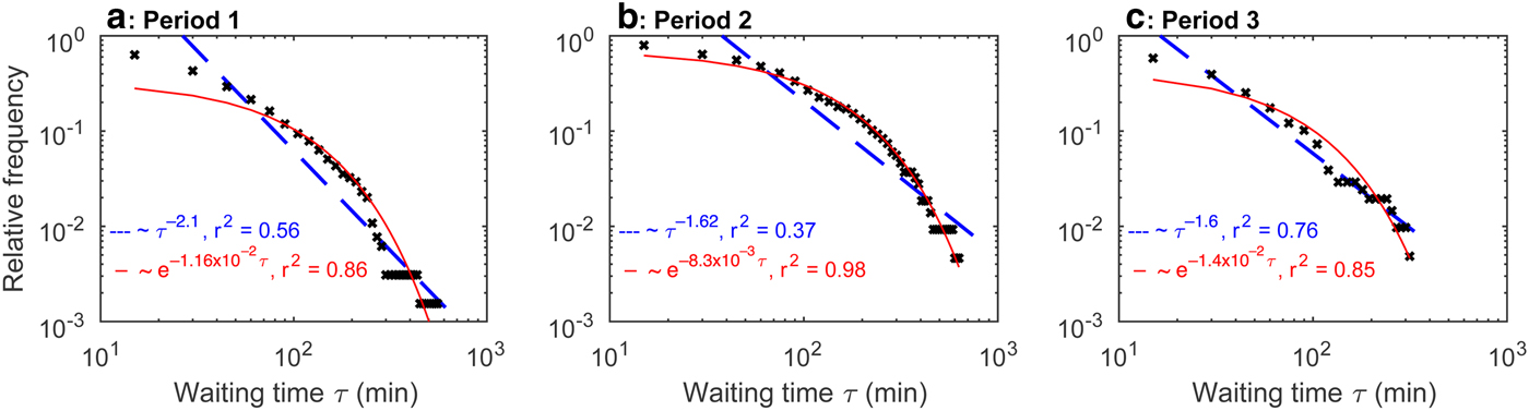
Fig. 8. Distributions of waiting times τ (with 15 min bins; log–log scale) in (a) period 1, (b) period 2 and (c) period 3. Blue dashed and solid red lines indicate best-fit power-low and exponential distribution.
4.3. Surface waves generated by subaerial and subaqueous calving
Figure 9 shows an example of surface waves generated by a subaerial-calving event (Drop), which was an ice tower break-off into the lake at the location 1310 m from the sensor (Figs 9a–c). The generated wave had a positive onset; its amplitude decreased gradually over five minutes after the maximum wave amplitude of 0.4 m (Fig. 9d). Low-frequency surface waves (~0.05 Hz) arrived first at the sensor, followed by higher frequency waves up to 0.2 Hz (Fig. 9e). This corresponds to the frequency dispersion of multiple-frequency waves as was previously reported by MacAyeal and others (Reference MacAyeal2006, Reference MacAyeal, Okal, Aster and Bassis2009) for micro-tsunamis observed in Antarctica. The wave had a peak amplitude at a frequency of 0.06 Hz, with relatively strong power between 0.02 and 0.15 Hz (Fig. 9f).
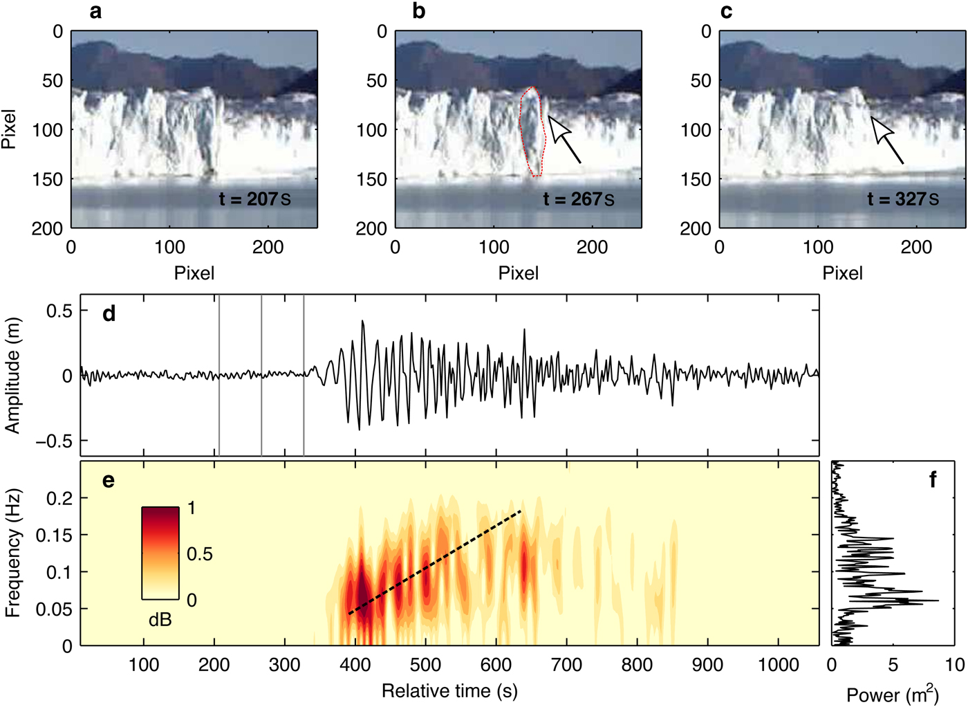
Fig. 9. (a)–(c) Time-lapse photograph sequence of a subaerial calving (Drop) which took place on 2 March 2016. The arrows indicate the main calving location and polygon shows an ice surface exposed after this event. (d) Surface waves generated by the calving, (e) spectrogram and (f) power spectrum. Gray vertical lines indicate the timing of images shown in (a)–(c). The dotted line highlights a relationship between the peak frequency and arrival time.
Figure 10 shows an example of a surface wave generated by a subaqueous-calving event that occurred at 960 m from the sensor. In contrast to the subaerial-calving event, surface waves generated by subaqueous-calving events had different characteristics in terms of amplitude and frequency (Fig. 10). The wave had no clear onset and its amplitude suddenly dropped by 0.3 m after the maximum amplitude of 0.4 m (Fig. 10d). Low-frequency wave arrived first (0.05 Hz) at the sensor. The dominant frequency was 0.11 Hz, and the power was concentrated between 0.1 and 0.13 Hz (Fig. 10f). The signal power was smaller than that of waves generated by subaerial calving. The waves did not have high-frequency content (0.13–0.25 Hz) compared with subaerial events (Figs 9e, 10e).
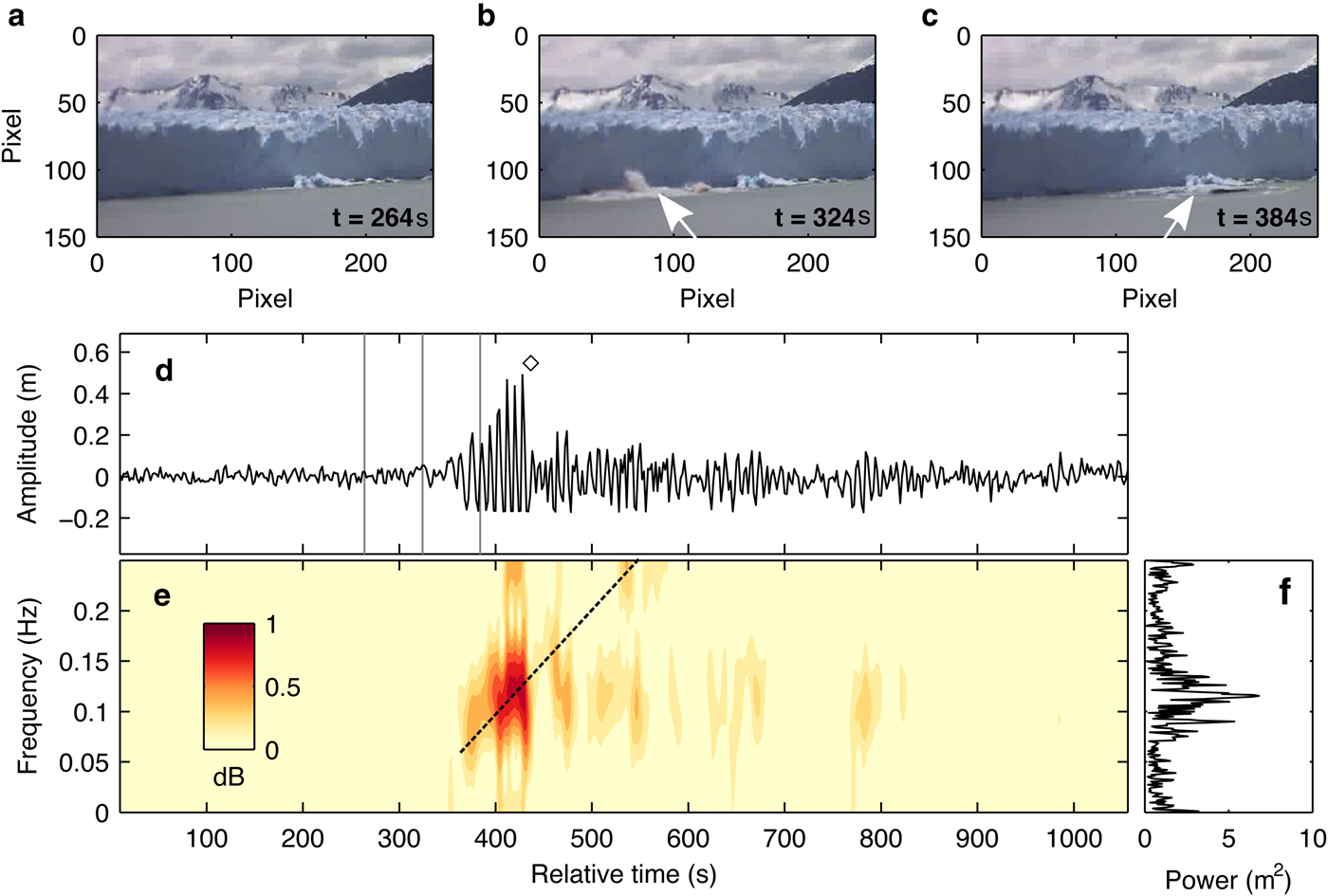
Fig. 10. (a)–(c) Time-lapse photograph sequence of subaqueous calving on 27 December 2013. (d) Surface waves generated by the calving (negative amplitude clipping was caused by a water-level drop below the sensor depth). The black diamond indicates the timing of sudden drop in the amplitude. (e) Spectrogram and (f) power spectrum of the surface wave.
5. DISCUSSION
5.1. Glacier calving at Glaciar Perito Moreno
The location of calving events was unevenly distributed in periods 1 and 2 (Fig. 3). Calving events clustered in ~700 and 1100–1300 m from the pressure sensor. The distribution seems to be controlled by the lake bathymetry in Brazo Rico near the ice front (Fig. 1). The lake bathymetry forms a relatively rugged basin (Fig. 1). The lake is 20–40 m shallower at ~700 and 1100–1300 m from the sensor, and the ice cliff is higher at this region by ~20 m (Fig. 1). Higher ice cliffs will lead to larger tensile stresses affecting calving activity (Hanson and Hooke, Reference Hanson and Hooke2003). In addition to this, gaps between crevasses are larger (Fig. 1), suggesting that the horizontal strain rate is greater in these regions. Most likely, these geometrical and dynamic conditions affect the observed location of the calving events (Fig. 3).
Only ten events (2%) out of 420 calving events occurred underwater (Table 1). The location of subaqueous-calving events was unevenly distributed (Fig. 3). For example, we observed subaqueous-calving events only at distances ~600, 1000 and 1200 m in period 1 where relatively larger number of subaerial calving was observed (Fig. 3d). It was suggested that as ice above the water level breaks off, overburden load counteraction to the buoyance decreases and subaqueous calving occurs (Van der Veen, Reference Van der Veen2002). Thus, a relatively large number of subaerial-calving events might trigger subaqueous calving at GPM. In addition to this, a number of subaqueous-calving events was substantially smaller than subaerial calving (Table 1). In GPM, a warm lakewater temperature ( ~9°C) was observed in front of the glacier compared with other proglacial lakes in Patagonia (Sugiyama and others, Reference Sugiyama2016). In fact, the latter study estimated that the magnitude of subaqueous-melt rate near the glacier front is ~7–33% of the ice speed. The low frequency of subaqueous-calving events may imply that subaqueous melting rate is similar to subaerial-calving rate at GPM.
On the time-lapse images, a greater number of calving events were observed in periods 1 and 3 than in period 2 (Fig. 4). Some calving events were not recorded by the cameras due to a lack of sunlight and blind angles, but results from pressure sensor and time-lapse cameras agree that events were more frequent in periods 1 and 3. The more frequent calving in periods 1 and 3 is associated with relatively warm air temperature. The mean air temperature over the periods measured near the glacier front was 8.5 ± 2.4 (±SD), 3.1 ± 1.9 and 9.7 ± 1.9°C for periods 1, 2 and 3, respectively. Minowa and others (Reference Minowa, Sugiyama, Sakakibara and Skvarca2017) investigated seasonal variations in the ice front position of GPM based on satellite image analysis. The glacier began to retreat typically in December and then turned to advance in April (Minowa and others, Reference Minowa, Sugiyama, Sakakibara and Skvarca2017). The seasonal ice front variations (±100 m) were controlled by frontal ablation, which varies from maximum in February to minimum in July. This seasonality is consistent with the number of calving events observed in this study (Fig. 4). The seasonal variation in the frontal ablation was correlated with lake and air temperatures, but not with the ice speed (Minowa and others, Reference Minowa, Sugiyama, Sakakibara and Skvarca2017), suggesting the importance of subaqueous melting and calving induced by waterline notch formation. Unlike the proglacial lakes in Alaska and New Zealand, where water temperature is cold (<1°C) (e.g., Röhl, Reference Röhl2006; Truffer and Motyka, Reference Truffer and Motyka2016), water is warm ( ~ 9°C) in front of GPM and temperature shows seasonal variations at all depths of the lake (Sugiyama and others, Reference Sugiyama2016; Minowa and others, Reference Minowa, Sugiyama, Sakakibara and Skvarca2017). Thus, we attribute the higher calving frequency in periods 1 and 3 to the relatively warm lake-water conditions, which enhanced the melting of the ice front and induced more calving.
For additional statistical characterization, we also computed interevent time interval between calving events. The obtained cumulative distribution of interevent time intervals can be well represented by exponential probability distribution, especially for period 2 (Fig. 8b). Yet, in periods 1 and 3, power law modeled the distribution also reasonably well (Figs 8a, c). There are several previous studies reporting the probability distribution of calving waiting time. On one hand, Åström and others (Reference Åström2014) reported that modeled and observed waiting-time distributions tend to follow power laws, suggesting that calving behaves as a self-organized system readily fluctuating in response to changes in climate and geometric conditions. Although, one of their studied glaciers, Yahtse Glacier in Alaska, did not follow a power law but could be fitted well with an exponential distribution. On the other hand, Chapuis and Tetzlaff (Reference Chapuis and Tetzlaff2014); Petlicki and Kinnard (Reference Petlicki and Kinnard2016) reported that waiting-time distribution follows neither an exponential model nor a power law based on their observations at ocean-terminating glaciers in Svalbard and Antarctic Peninsula. Our results are in line with those observed at relatively small and grounded Yahtse Glacier in Alaska, implying that the events at GPM occur randomly in time.
5.2. Source-to-receiver distance
One possible application of surface waves data collection is the estimation of the source-to-sensor distances, which was previously applied in Antarctica, but not validated with data (MacAyeal and others, Reference MacAyeal, Okal, Aster and Bassis2009). Source-to-sensor distance can be used to locate calving events, which would help to better understand driving mechanisms of calving. For deep-water waves, the arrival time of a surface wave can be assumed as linearly dependent on the wave frequency (MacAyeal and others, Reference MacAyeal, Okal, Aster and Bassis2009). Therefore, Eqn (3) allows us to estimate the source-to-sensor distance from surface-wave observations alone (MacAyeal and others, Reference MacAyeal, Okal, Aster and Bassis2009).
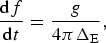 $$\displaystyle{{{\rm d}f} \over {{\rm d}t}} = \displaystyle{g \over {4\pi \Delta_{\rm E}}},$$
where t is the arrival time of a wave with a frequency f. Equation (4) is used to determine distance ΔE from the measurements of df/dt that were obtained by fitting a linear relationship to the peak frequency in spectrograms (Figs 9, 10). First, we obtained peak frequency by calculating power spectral density repeatedly with the data window of 5–20 s with a 1 s time step (Figs 11a, b). Then, we performed linear regression, weighted by the power of the peak frequencies, to obtain df/dt and the SD. Weighted linear regression was performed again after excluding outliers deviated by more than one SD. Finally, we calculated its qualities of fitting (r 2) as an index to evaluate ΔE (Fig. 11b). We analyzed 137 cases distributed over periods 1–3 to compare the distance estimated using the above explained method and measured with the time-lapse and satellite imagery (Fig. 3). The mean r 2 of the entire sample of linear regression lines was 0.71 with an SD of 0.25.

Fig. 11. (a) A waveform generated by a calving event (19 December 2013 11:38–11:44) as an example of the data used for the analysis. (b) Spectrogram of the wave shown in (a). Gray crosses and green circles are peak frequencies calculated with 5 and 20 s data windows, respectively. Gray and green dashed lines are weighted linear regression of the peak frequency. (c) Scatter plot of measured ΔM and estimated ΔE source-to-sensor distances. Marker color and type indicate coefficient of determination of the regression lines and observation period, respectively. The black line and gray dashed lines indicate 1:1 correspondence and relative error of estimated distance, respectively.
By visual inspection of Figure 11c, the reader will observe that the estimated source-to-sensor distance agrees well with the observation within ~20%. The RMSE of the estimated distance against the observation was 300 m. The accuracy of the estimation is dependent on the wave magnitude at the peak frequency relative to the background noise. More reliable estimation is possible by increasing the number of pressure sensors. The deep-water condition assumed in the above calculation requires that the condition h/L >0.5 is satisfied, where the wavelength L = g/(2π)T 2, with t and g standing for wave period and gravitational acceleration, respectively. Considering the lake depth near the calving front (60–100 m) and the dominant wave period of 9 s, the study site places it almost at the threshold of the deep-water condition (8.8–11.3 s). Combining this important background with the fact that the dispersion was actually documented, we may assume that the accuracy of the source-to-receiver distance could be affected by travel path. However, sensitivity tests with high-pass-filtered waveforms (i.e., when we analyze only waves with periods shorter than the threshold) did not yield any obvious improvements. Finally, we note that if lakes and fjords in front of glaciers are too shallow, the method proposed here may not be applicable.
5.3. Frequency characteristics of calving styles
To understand the relationship between calving styles and properties of surface waves more clearly, as well as statistically, we performed spectral analysis of 420 surface waves, for which calving styles were categorized based on time-lapse images. Obtained power spectra were averaged for each calving style and normalized by the maximum power before the comparison. Our data demonstrate that subaerial- and subaqueous-calving events generate waves with different characteristics, suggesting either that (i) waveforms and frequencies of waves are dependent on the calving style, or (ii) the difference is due to path effects (Fig. 12).

Fig. 12. (a) Power spectra of the waves generated by the four different calving styles. Each solid curve obtained by taking the mean of all events categorized as each style with a sample number indicated in the legend. The shade indicates standard error distribution of the data. Gray line indicates power spectra of background noise for 100 min wave record. (b) Power spectra of the waves generated by the Drop calving styles with different distances from the pressure sensor.
All of the calving-generated surface waves show a peak frequency ~0.11 Hz (Fig. 12a). While the number of subaqueous-calving events was limited compared with subaerial-calving events, waves generated by subaqueous calving were characterized by a lack of high-frequency waves between 0.12 and 0.25 Hz, and the peak frequency power was more pronounced compared with subaerial calving (Fig. 12a). This difference could be explained by scales associated to iceberg detachment from the glacier front. If subaerial calving produces smaller icebergs and splashes of different sizes, the associated impacts are supposed to generate higher frequency waves. According to our time-lapse images, subaqueous calving is characterized by a single, relatively large iceberg floating up to the lake surface. Thus, spectral differences could be related to a difference of scales, which, however, is difficult to verify by visual inspection of time-lapse photographs due to largely unseen volume of subaqueous icebergs.
Slightly different frequency distributions were observed among the three subaerial-calving styles: Serac, Drop and Topple (Fig. 12a). In general, surface waves after Topple and Serac style events had greater power in the lower (e.g., ~0.06 Hz) and higher frequency bands (e.g., ~0.23 Hz), respectively. These results are consistent with a modeling study of Massel and Przyborska (Reference Massel and Przyborska2013), which suggested that longer and shorter period waves characterize those generated by Topple and Serac events.
The presented frequency difference was observed repeatedly and visible in averaged spectra for ten-to-hundreds events (Fig. 12a). However, the spectral differences between calving styles could be simply generated by path effects, in particular by faster attenuation of high-frequency waves with distance. To asses this possibility, we calculated normalized power spectra of several Drop-type calving events taking place at different distances (Fig. 12b). Such analysis suggested: (i) first, that the dominant period remained the same at different distances, confirming that the peak frequency of tsunami signals were not significantly affected by the distance; (ii) second, that at distances larger than 1 km, high-frequency energy between 0.12 and 0.25 Hz can be reduced (Fig. 12b). Closer events had 10–20% higher power at the higher frequencies. This indicates that high-frequency waves may attenuate more with distance while low-frequency waves do not. Considering a lack of subaquaous-calving events at shorter distances, and an abundance of subaerial events at close distances (Fig. 3), path effects can be responsible for spectral differences shown in Figure 12a. The above-mentioned analysis implies that even if spectral differences between subaerial- and subaquaous-calving exist, it can be difficult or impossible to classify distant events.
Finally, it is interesting to asses a possibility of distorting interference of local bathymetry and path effects on the dominant period of the presented tsunami spectra. It is well known from research on tsunami source reconstruction, that near-shore tsunami records can be determined mainly by local topography effects. According to Rabinovich (Reference Rabinovich1997), the key approach to separate such influence is based on comparative analysis of tsunami and background noise spectra. Many observations show that background and tsunami spectra were generally in good agreement, meaning that the tsunami record is influenced by the natural resonance of the tide gauge neighboring topography. We check if such distorting influence appears in our records by computing the spectra of noise (for a quiet time interval of 100 min without calving events) and comparing it with the spectra of calving events (Fig. 12). This analysis shows that noise is relatively broadband and does not have obvious peaks which could correspond to seiches or maximum amplitudes produced by micro-tsunamis, and therefore, suggests that a possibility of local interference of local bathymetry is insignificant.
5.4. Iceberg size and wave properties
One of the practical applications of surface-wave measurements is the estimation of iceberg volume released by calving events. Recent studies endeavor to estimate calving flux by using seismic and acoustic signals (Bartholomaus and others, Reference Bartholomaus2015; Glowacki and others, Reference Glowacki2015). In order to explore the relationship between iceberg volume and wave properties, we estimated the volume from the time-lapse images and compared it with median frequency and maximum height of the wave. Geometric attenuation in the surface-wave amplitude (e.g., Podolskiy and Walter, Reference Podolskiy and Walter2016) was taken into account by multiplying the wave height with  $\sqrt {\Delta _{\rm M}} $, where ΔM is the measured distance to the source. In total, 92 events observed over the three periods were considered for this analysis (Fig. 13a). Ice surface area (A C) exposed after the calving was manually quantified by comparing images taken before and after the subaerial-calving events (e.g., Fig. 9 red line). We converted the unit of A C from image scale pixel to real world scale m by using a relationship $f_{\rm l}^2 /A_{{\rm C}\_{\rm img}} = d^2/A_{{\rm C}\_{\rm real}}$, where f l and d are the focal length of the camera (5.01 mm) and a distance between the cameras and calving locations, respectively. Sensor size of the time-lapse camera was 6.4 × 5.1 mm (1 px = 5 µm). d was derived from manual comparison between Landsat imagery and the time-lapse photographs using easily discernible features. We used only images taken by cameras 2, 3 and 4, which were oriented more perpendicular to the ice front (Figs 3h–j). Iceberg volume was then calculated by $V_{\rm C} = CA_{\rm C}^{3/2} $, by assuming that the depth of the calved ice is proportional to the square root of newly exposed area. C is a constant scaling factor that is found to be ~0.12 (Åström and others, Reference Åström2014; Petlicki and Kinnard, Reference Petlicki and Kinnard2016). The assumption is supported by previous observations of ocean-terminating glaciers in Svalbard (Dowdeswell and Forsberg, Reference Dowdeswell and Forsberg1992) and was successfully applied for studying a ocean-terminating glacier in Antarctica (Petlicki and Kinnard, Reference Petlicki and Kinnard2016). The accuracy of V C is difficult to estimate because the exposed ice surface is not perfectly perpendicular to the sight of the camera and the iceberg shapes are irregular. If we assume 10% of error bound in $A_{{\rm C}\_{\rm img}}$ and d, and each of these uncertainties are independent, an error associated with the image analysis is 30%.
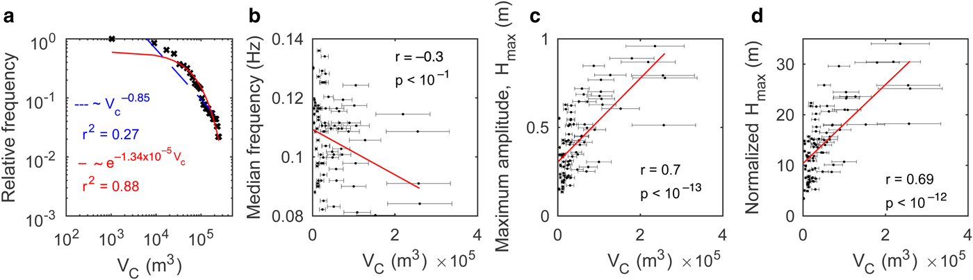
Fig. 13. (a) Distribution of iceberg size V C (with 8 × 10³ m3 bins; log–log scale). Blue dashed and red solid lines indicate best-fit power-low and exponential distribution. Scatter plots for iceberg size versus (b) median frequency, (c) maximum amplitude and (d) maximum amplitude corrected for source-to-sensor distance  $\Delta _{\rm M}({\rm i.e.,}\; H_{{\rm max}} \times \sqrt {\Delta _{\rm M}} )$.
Figure 13a shows a cumulative distribution function of iceberg volume V C. The observed distribution was modeled by best-fit power-law and exponential models. The iceberg volume ranged from the minimum of 1.04 × 10³ m3 to the maximum of 2.6 × 10⁵ m3, with a mean V C equal to 4.9 × 10⁴ m3. These numbers were consistent with the previous studies on relatively small, grounded ocean-terminating glaciers in Alaska, Svalbard and Antarctica (Bartholomaus and others, Reference Bartholomaus, Larsen, O'Neel and West2012; Chapuis and Tetzlaff, Reference Chapuis and Tetzlaff2014; Petlicki and Kinnard, Reference Petlicki and Kinnard2016). However, compared with these previous studies, the distribution of iceberg volume could be better reproduced by an exponential model than by the power law (Fig. 13a). Among possible reasons for this disagreement are: a small sample size (n = 92) or some real physical difference between calving at ocean-terminating and lake-terminating glaciers (e.g., Benn and others, Reference Benn, Warren and Mottram2007), which remains to be clarified by future studies.
A relationship was observed between the iceberg size and the maximum amplitude of the surface waves (Fig. 13). Median frequency showed slightly negative relationship, and maximum wave amplitudes and their normalized values showed positive relationships with the iceberg size. Intuitively, one can expect that there may be a negative relationship between frequency and iceberg size; i.e., it is reasonable to speculate that small iceberg calving (Serac) tend to have their peak frequency at a higher frequency, while larger calving styles (Topple and Drop types) tend to have it at the lower frequency. Nevertheless, there is inconclusive evidence about the significance of the correlation between the median frequency and the iceberg volume (Fig. 13b). This could suggest that: (i) the distribution of iceberg sizes was too limited due to the site conditions to observe a wide variation of the dominant frequency; or alternatively, (ii) be caused by path effects (i.e., effects from lake topography). Contrary to the median frequency, we observed a clearer relationship between maximum amplitude and size (Figs 13c, d). Since maximum amplitude decays with distance, we expected a positive relationship would become clearer if we compare normalized maximum amplitude with iceberg size. However, the effect of normalization was limited. There are some data which do not fit the linear regression (Figs 13c, d). To investigate how sensitive this relationship is to outliers, we excluded those deviated by more than one SD and performed linear regression again. The linear regression model changed only 5.2 and 5.4% from the original regression models. Thus, the effect of the outliers was limited. These results indicate that maximum wave amplitude has a potential to be used as a proxy for the calving flux. However, to find a quantitative relationship between the calving flux and surface waves, we need to quantify iceberg size more precisely by analyzing high-resolution digital elevation models.
5.5. Comparison with Antarctic micro-tsunami
MacAyeal and others (Reference MacAyeal, Okal, Aster and Bassis2009) recognized that seismic observations of glaciogenic ocean waves (micro-tsunamis) are useful for studying calving and other processes of ice shelves in Antarctica. Over a 3-year observation, seismometer arrays on the Ross Ice Shelf and several icebergs recorded 368 impulsive events with a duration between 1 and 30 min and dominant frequencies of 0.05–0.2 Hz. These local ocean-wave signals were attributed to a wide range of glaciological sources, such as small-scale calving, iceberg capsizing and collision, rift propagation, tidal ice motion in the grounding zone and submarine landslides. Surface waves observed in front of GPM had similar duration and spectral properties to those documented by MacAyeal and others (Reference MacAyeal, Okal, Aster and Bassis2009). Iceberg calving was suggested as the most likely source of wave-arrival events in the coastal Antarctic waters (MacAyeal and others, Reference MacAyeal, Okal, Aster and Bassis2009). Our ground-validated analysis (and clear association of surface-wave signals with calving) confirms their hypothesis.
Furthermore, MacAyeal and others (Reference MacAyeal, Okal, Aster and Bassis2009) computed source-to-receiver distances for the events in their catalog by using the dispersion relationship at deep-water limit. The obtained values corresponded to distances from ~10 to 700 km. Similar method employed in our study yielded two-orders-of-magnitude shorter distances, which agreed reasonably well with the results of time-lapse imagery.
Finally, we note that in the ocean, background noise can increase due to trans-oceanic sea swell, which makes detection of glaciogenic waves in the sub-0.15 Hz range impossible (MacAyeal and others, Reference MacAyeal, Okal, Aster and Bassis2009). From this perspective, a lack of time periods with such noise makes the discussed methodology more useful at lake-terminating glaciers. In general, we conclude that the pioneering idea to focus on micro-tsunami signals (MacAyeal and others, Reference MacAyeal, Okal, Aster and Bassis2009) will continue to be useful in the study of iceberg-calving.
6. CONCLUSIONS
We observed surface waves generated by calving events using a pressure sensor installed in front of a lake-terminating glacier in Patagonia. The surface-wave measurements were accompanied by time-lapse photography to record the locations and styles of calving. During three field campaigns over 39 d in total, we counted on photographs 420 calving events, which were dominated by subaerial-calving style (98%). The events were non-uniformly distributed along the ice front because calving occurred more frequently at the region characterized by shallow bathymetry and large gaps between crevasses. Comparison of time-lapse images and surface-water wave measurements shows that iceberg calving generates waves that are distinct from local noise, such as tourist boats and wind. This allowed us to count 1074 calving events from surface-wave records, including those that were not observable by the camera. The data indicate that calving events took place ~2.6 times more frequently in December and March (austral summer) than in October (austral spring), while calving front position remained relatively stable between the considered periods. The distributions of calving-interevent time and iceberg size appear to be exponential, but it remains to be understood if this can be called a prominent feature of lake-terminating glaciers or not.
Interestingly, waves generated by subaerial and subaqueous calving showed similar frequency dispersion, which is common only for the so-called deep water. To assess the potential to use surface waves for glacier-calving monitoring, we estimated source-to-sensor distance by assuming a linear relationship between wave frequencies and their arrival time at the sensor. The results agreed with the distance measured by the time-lapse images within ~20% errors. Our analysis also suggested that waves generated by subaqueous calving are characterized by a lack of power between 0.12 and 0.25 Hz. However, considering that most of the observed subaquaous events were relatively far from the receiver, attenuation of high-frequency energy could be responsible for such feature, meaning that it remains to be clarified by future research if power spectrum of surface waves really depends on the style of calving. Finally, we found relationships between calving volume estimated from time-lapse images and maximum amplitude. Therefore, our study demonstrated a potential to monitor the occurrence, location and volume of calving events with a relatively simple surface-wave measurement.
Long-term monitoring of calving by means of surface-wave measurements should help to better constrain the driving mechanisms of calving at GPM and other glaciers. Due to the complexity of effects from local bathymetry and wave paths (both at the source and receiver locations) on waveforms, further investigations are needed to improve the results explored in this paper. For instance, an open question about an existence of a robust relationship between iceberg volume or type and waveforms could be addressed with accurate measurements of iceberg volume and modeling in future studies.
CONTRIBUTION STATEMENT
M.M. analyzed data, made the figures and wrote the paper. E.P. contributed to the analysis of waveforms and dispersion and wrote the paper. S.S. designed the field activities at the glacier and contributed to writing the paper. M.M., S.S., D.S. and P.S. contributed to the fieldwork. All authors contributed to the discussion of the results and participated in the writing of the paper.
ACKNOWLEDGEMENTS
We thank Y. Ohashi, T. Sawagaki and N. Naito for their help in the field. Special thanks to Hielo y Aventura for logistical support. The manuscript was improved by comments and suggestions from M. Truffer, and handled by Scientific Editor, Hamish Pritchard, and carefully commended by Martin Lüthi and an anonymous reviewer. This research was supported by the Japan Society for the Promotion of Science; Grants-in-Aid for Scientific Research JP23403006, JP26550001 and JP16H05734; Grant-in-Aid for JSPS Research Fellow JP16J01860; and by the Inoue Found for Field Science of the Japanese Society of Snow and Ice. Landsat images were downloaded from http://earthexplorer.usgs.gov/.


 Open access