


I. Introduction
This report describes the results from the installation of three continuously recording Cambridge-type wire strainmeters on the surface of the Barnes Ice Cap, Baffin Island, Canada $$$(lat. 690 45' N., long. 72° 15'W.). $$$The strainmeters were installed along an approximate flow line, where pole arrays had been previously set up, 10.6 km and 19.5 km from the ice divide (Fig. 1), in order to study the flow in a region which was known to have undergone a surge (Reference HoldsworthHoldsworth, 1973). At the 19.5 km location, a 50 m gauge-length strain array was set up beside two strainmeters separated by 120 m along the flow line (Fig. 2). At the 10.6 km pole, a single 50 m strain line was set up (Fig. 3), approximately parallel to the flow line. The 50 m gauge lengths and the 1 km distances (set up in 1974) were remeasured every three to twelve days (Fig. 4).
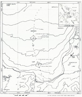
Fig. 1. The location of the strainmeter sites on the Barnes Ice Cap, Baffin Island.

Fig. 2. The 50 m pole array, and the location of the two strainmeters (120 m apart, units 1 and 2) at the 19.5 km pole.
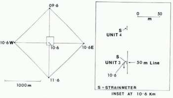
Fig. 3. The 50 m line and t'tr relation to the two strainmeter sites (units 3 and 4) at the 10.5km pole.

Fig. 4. Data collection schedule, April and May 1976. Units 1-4: 5 m wire strainmeters; A : 50 m strain array at 19.5 km; B:50 m strain line al 10.6km; C: 1 km line, 9.6km to 10.6km; D: 1 km line, 10.6km to 11.6km.
The experiment was designed first to complete an evaluation of the use of wire strain-meters for the rapid determination of surface strain-rates on large ice masses, secondly to compare strains over different gauge lengths (5 m, 50 m, and 1 km) in order to sample the coherence of the surface strain-rates, and thirdly to see if the nature of the strain-rates could indicate something about the basal conditions (smooth versus jerky motion). A wire strain-meter of this particular design had only once before been used to measure surface strains on a glacier (Reference Goodman, Goodman, Allan and BilhamGoodman and others, 1975; Goodman, unpublished). Previously, the use of wire strain gauges has been reported, e.g. by Reference Meier and MeierMeier and others (1957) and Reference Warner, Cloud and RossiWarner and Cloud (1974) but these gauges were of the electrical-resistance type.
The present site was chosen because ice strain, movement, temperature, and depth data were already available, the mean air temperature for mid-April to mid-May was known to be well below o°CFootnote * (thus reducing regelation problems) and the ice surface was only covered by about 1.0^ 0.30 m of snow.
The experiment was carried out jointly by the Glaciology Division of the Department of the Environment, Canada, and two departments of the University of Cambridge (Geodesy and Geophysics and Cavendish Laboratory), U.K. The field party (K.E. and G.H.) collected strain data from 24 April to 15 May 1976.
2. Instrumentation
2.1. Strainmeters
Three modified Cambridge-type wire strainmeters were used. The modifications increased the maximum recordable strain to 2 X to-3 while maintaining a resolution of about to-8 strain. $ The strainmeters used 5 m of Invar wire as a length standard. The wire was kept under constant tension, and hence length, by a lever and weight system. Lever rotation, which is proportional to strain, was measured with an inductive displacement transducer. The output from the transducer was amplified and recorded on a Rustrack recorder. The signal was automatically re-zeroed both electronically and mechanically so the instrument could be left at a high sensitivity (8xiO-7 strain full-scale deflection, 120 mm chart width) unattended without loss of data. The instrument layout is shown in Figure 5. A trench, 1 m wide, was dug in the snow until ice was reached, and in each case a strip of ice, 6 m in length, was selected which was free of visible cracks. Some of these cracks ran close to, but never crossed, a strainmeter installation.
The strainmeters were installed in the base of the snow trenches which were from about 0.8 to 1.2 m deep (Fig. 6). Each PVC baseplate was fixed to the ice with four 20 cm and 40 cm long tubular ice screws, augcrcd into pre-drilled, 1.5 cm dia. holes in the ice. Water was poured around the plate edges and allowed to freeze. The wire was enclosed within 5 m of 2.5 inch (6.35 cm) dia. aluminium tubing fitted with neoprene rubber bellows couplings. The tension in the wire was brought down to 8 N to minimize regelation effects (for which there was no evidence). Several days' data were lost because of low capacity and voltage of lead-acid accumulators at the ambient temperatures. Catalytic paraffin heaters were used later in the experiment, but ventilation problems precluded their effective use. Alternative power sources would lead to greater expense.
Except for brief periods, the temperature and pressure were continuously recorded in the trench of the strainmeter at the 19.5 km site (Fig. 6). The large strain-rates observed (Fig. 7) seem to dominate any temperature-induced changes in the wire. No correlation between temperature and strain is apparent on a daily basis (Fig. 8). The larger fluctuations in trench temperature at the beginning of the experiment occurred because the trench was not completely back-filled. Heavy drifting in early May filled the trench and hence attenuated subsequent temperature fluctuations.

Fig. 5. Two photographs of the strainmeter tensioning unit, and mechanical re-zeroing system.

Fig. 6. A schematic diagram of a strainmeler installation on the ice cap.

Fig. 7. Part of the record from the strainmeter. The offsets are automatically introduced to keep the signal within the range of the chart recorder.

Fig. 8. Daily mean strain rates calculated for the digitized records from each strainmeter.
2.2. Pole arrays
For the 50 m array, 3 m by 38 mm dia. aluminium tubes (3.2 mm wall thickness) were used for poles, approximately 1 m in snow and approximately 1 m above the surface. Measurements between reference pins mounted on top of the poles were made with a "LOVAR" tape (Keuffel and Esscr ser. No. 720408) suspended in catenary using a 15 kg weight on a trestle at one end and a pivot arm (straining bar) for zeroing the tape, at the other end. The mean of three readings (recorded to within 0.1 mm) was taken for each observation. When the temperature correction had been made, both end readings were estimated to be accurate to ±0.2 mm, allowing for unquantified errors such as produced by wind impinging on the tape. Thus the total distance error is taken as $$+o.4 mm.
Distances between the stakes 1 km apart were measured with a Wild DI-10 Mk 1 1 I.R. Distomat (standard error 15 mm). Six to eight readings were taken for each distance and meteorological corrections applied to the mean.
2.3. Note on cracks in the ice
Cracks of up to 1 cm width, and exhibiting progressive opening, were observed. The snow-pack was split above most cracks, indicating opening during the winter. These cracks may thus be called crevasses although their orientation tended to be variable, especially for the trace of an individual crack. In early summer, these cracks must be sealed by superimposed ice, so their existence is quite temporary. Crack spacings were of order 5 m, so that the 50 m and larger strain lines intersected these cracks frequently. Since only spot observations were made on cracks, a description of their geometry is not possible. Irregular strains recorded at these sites may have been caused by crack activity.
3. Results
3.1. Strainmeters
An example of the chart trace from one of the Rustrack recorders is shown in Figure 7. The steps produced by the automatic re-zeroing were removed when the chart was digitized. A time series, with 0.25 h time step, was produced from the digitization and this has been replotted. Means of strain-rate on a roughly daily basis were also calculated from the time sequence.
Data were obtained from the strainmeter at the 10.6 km pole (Unit 3) between 2 and 14 May. A plot appears in Figure 8 and Table 1 gives the mean strain-rate values.
Table I. Mean Strain-Bates: Unit 3* (10.6 Km Site)

Data from Units 1 and 2 (at the 19.6 km pole) were digitized for the periods 2 May to 11 May for Unit 1, and 23 April to 4 May, and 7 May to 15 May for Unit 2. The observed strain is plotted in Figure 8 and the daily means appear in Table II.
Table II. Mean Strain-Rates: Unit I (120 m from 19.5 km Polk)

In all three cases the daily mean strain-rate slowly fluctuates. When the daily means are plotted (Fig. 8) there appears to be a quasiperiodic trend with a period of about 11 d although the data sequence is hardly long enough to enable any definite conclusions to be made. There appears to be an approximately 9 d phase lag between Units 1 and 2 (it is assumed a wave is propagating down the flow line).
The observed periodicity in strain-rates might be due to varying thermal stresses in the ice controlled by the altering, by the snow cover, of the surface temperature fluctuations (Reference SandersonSanderson, 1978; personal communication from C. S. M, Doake).
3.2. Pole array results
The days on which measurements were made are shown in Figure 4, and Tables III and IV give the results for the various arrays.
In most cases a constant strain-rate has been assumed and calculated by linear regression. The scatter m the results from the 50 m arrays is particularly large. The main uncertainties m the length values lie in the temperature correction (an extrapolation of the coefficient of expansion was taken to apply at these temperatures) and the result of the force due to wind blowing on the tape suspended in catenary. The latter effect may have caused a transitory incorrect tension in the tape on some occasions. However, these sources of error are not considered sufficiently large to explain the very erratic nature of the length changes, and we tentatively suggest that the cracks in the ice may be largely responsible for this.
Table III. Poll; Array Results: 10.6 km Strain Station

Table IV. Poliî Array Results: 19.5 km Strain Station


Fig. 9. The pole data for the 10.6 km diamond.

Fig. 10. The strain data from the 10.6 km diamond and 50 m line while the site was occupied.
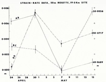
Fig. 11. The 50 m rosette data at the 19.5 km site.
For the 19.5 km (50 m gauge length) strain array, we have taken the strain-rates obtained from linear regression of the readings for each leg to compute the three strain-rate components. Using Kehle's equations (Reference Zumberge, Zumberge, Giovinetto, Kehle and ReidZumberge and others, 1960) for computing principal strains from such an array (see Appendix A) we obtain :

with the principal extension axis inclined at $28.90 to the west of BC (approximately parallel to the strainmeter, and hence the main pole line (see Fig. 1)). The strain-diamond data at 19.5 km (Appendix B) was analysed using the method of Reference NyeNye (1959) and the results for 1974-75 are:

with the principal extension axis inclined at 31.8° to the west of the main pole line direction (i.e. 19.5 km -> 18.5 km) which is within $ 30 of the direction of $ BC of the 50 m strain array. Such an agreement in orientation of the two principal strain-rates suggests the data may be reliable. However, the magnitudes of the principal strain-rates differ by up to 14%. This could be related to the fact that the gauge length in the two instances differ by a factor of about 40. It should be noted that the cracks (crevasses) observed at 19.5 km in the immediate vicinity of installations tended to be irregular in orientation and not generally parallel to the indirection, suggesting that the cracks may be formed as a result of thermal stresses combined with regional How stresses. The origin of the apparent jerky strain in the 50 m array is possibly related to crack activity although it is conceivable that we have overlooked some additional errors in the tape measurements.
If the 50 m strain-array data are reworked using distances reduced to the horizontal (and thus strictly allowing them to be compared with the data from the strain diamond) we find that the principal strains are changed only by 0.8 to 2.5% and the orientation of the principal axes by O.09; therefore in the present case we may compare the large strain-array results (which are reduced to the horizontal) with the 50 m slope strain data without serious error. At the 10.6 km site we have again analyzed the strain-diamond data by the method of Reference NyeNye (1959) (Appendix B) and the results for 1974-75 are:
with the principal extension axis inclined at 40.7° west of the line 10.6 -> 09.6 km. These values apply to the horizontal plane. The large deviation between the flow direction (approximately in the line of the poles spaced at 1 km intervals) and the principal strain direction, implies large horizontal shear strains. We associate these with the surge and the existence of foliation in the ice (Reference HoldsworthHoldsworth, 1973).
3.3. Comparison of the two techniques
At the 10.6 km strain site, there appears to be reasonable agreement between the strain-meter results and the pole-array results. Thus the strainmeter gives 2.63 X lo^d >; the 50 m line gives between 2 and 3X 10"6d' depending on the interpretation of the results, and the 2 km X 1 km array (2.63 to 5.74) X io"6 d"> on two separate legs averaged over a two year period (assuming a linear variation of the strain-rate down the flow line).
At the 19.5 km site the two sets of results are not in good agreement. Data from the two strainmeters agree closely with each other (approximately $ 8x10-« d"1) but not with the strain-rates determined parallel to the instruments from the 50 m pole array $(3.3 X io"6 d ') or the 1 km pole array (2.3 X to6 d"!). $$ Although the 50 m pole data are questionable because of the large variations about the mean and the small number of data points, the 1 km data arc acceptable and may be compared with the strainmeter results provided seasonal or yearly fluctuations in strain-rates are small. Thus the discrepancy between the strain-rates measured over the 1 km and 5 m gauge lengths is probably real. If the strainmeters were not perfectly aligned with the 18.5 -» 19.5 line then some small discrepancy would be expected (Appendix A) but the strainmeter values exceeded the principal strain-rates derived analytically from the pole array data (Appendix B). The surface relief is much more pronounced at the 19.5 km site than the 10.6 km site, and whereas the latter is certainly underlain by ice at the pressure melting point, the former site is possibly in a region of transition from melting to freezing (Reference ClassenClassen, 1977) and this condition might also contribute to the somewhat irregular nature of the strain there, although this is not reflected in the strainmeter results.
4. Conclusions
The three continuously-recording wire strainmeters were successfully installed on the surface of the Barnes ice Cap and gave useful results after only a few hours of recording. The strainmeters could in principle be used to detect the passage of a kinematic wave or changes in surface strains due to thermal stress fluctuations. For these levels of strain-rate, $ « 10 s to 10-* d"1, $ this type of strainmeter is superior to the laser interferometer which has been used to detect similar magnitudes of strains in comparable periods of time (Reference HoldsworthHoldsworth, 1975}. The cost of the wire strainmeter is substantially less than that of the laser interferometer and the set-up time is only in the order of hours. A resolution of io~6 strain d"[ is easily achieved. The surface chosen for the installation, 1-1.5 m of snow on solid ice at well below melting point, proved ideal. Obvious difficulties are likely to be encountered with mounting the instruments on firm When there is no snow cover, the trench should be dug deeper than the estimated summer ablation. The strainmeters should normally be used in arrays of three so that the direction of the principal strain axes can be determined. This would have been done if more instruments and sufficient time had been available to us.
The comparison with the pole arrays at the 10.6 km site is good, implying that there, strains over two orders of magnitude in gauge length are relatively homogeneous, but at the 19.5 km site, significant differences occur between the strainmeter results and the pole-array results The differences can neither be accounted for by a change of calibration of the strainmeter nor by appealing to further significant errors in the longer-distance measurements. Therefore, we conclude that the differences are probably real and related to the flow regime there. Reference Colbeck and EvansColbeck and Evans (1971) observed on the Blue Glacier, U.S.A., that short (3 m) gauge lengths are in general not appropriate for studying gross glacier-flow problems.
Over 50 m gauge lengths, strain changes observed are due to opening or closing of cracks and creep; for the 5 m gauge lengths, where no cracks cross the strain wire, strain changes result from creep alone.
8. Acknowledgements
The Royal Society of London provided a grant which enabled the strainmeters to be purchased and freighted to the site. D.J.G. acknowledges the support of the Science Research Council and K.E. the support of the Natural Environment Research Council for research studentships. We thank G. Ballard for his help in preparing the instruments, E. Weaver for assistance in the field and Dr G. King for helpful discussions.
Appendix A Strain-Rate Results From 50 m Rosette At 19,5 km

Fig. a1. The direction of the principal strains at the 19.5 km pole.
the strain rosette was set out as shown in Figure A-1 on 20 April with 50.00 + 0.08 m legs at angles of$$$$ 1200 00'00"+13”. A subsequent angular check (30 April) showed that the angles 1 and 2 had changed only between 2" and 16”. The distances were measured four times (Fig. 4) and showed erratic changes. Performing a least-squares fit on the data, the strain-rate components in the three directions are:
and
Using Kehle's method (Reference Zumberge, Zumberge, Giovinetto, Kehle and ReidZumberge and others, 1960), the principal strain-rates are:
lf the first and final readings are used to calculate the (slope) strain-rate components, we obtain;
Reducing to the horizontal changes these values by less than 3%. That is, the principal strain-rates are within 3 to 22% of the strain-diamond values and the orientation within $$$30. The strain-diamond values are easily the most accurate of the two sets of data, so the fairly close agreement suggests that the rosette strain-rates may be reliable and that strain-rates are roughly homogeneous over scales of 50 to 2 000 m. However, there is no basis for claiming per se that strain-rates should remain relatively homogeneous down to 5 m gage lengths (see also Reference Colbeck and EvansColbeck and Evans, 1971 ).
Variation of strain-rate with orientation
We examine the variation of strain-rate at the 19.5 km site as a function of orientation. For analytical convenience and brevity we take a strain ellipse defined by
so that we avoid the more complicated analysis of the strain ellipsoid. For the present purposes, the error introduced by doing this is negligible. Following the notation of Jaeger {1962, p. 29) in his analysis of finite homogeneous strain in two dimensions, A, the relative length of the major axis after, say, one year is given by
and B, the relative length of the minor axis after one year is given by
The angle the lines of zero strain make with the major axis direction $$$ is ± S, given by
Therefore, the expected change in extending strain-rate with rotation is about $$$ 4.45 X 10⁻⁵ a-1$$$ per degree of are, on average.
It can thus be seen that a misorientation of 1° between the wire strainmeter and the pole lines would only change the strain-rate that is measured, by a trivial amount.
Appendix B 10.6 km and 19.5 km strain pole arrays (1974-75 Data)

Fig. b1. The directions of the principal strains at the 10.6 and 19.6km poles.
The two, nearly identical, strain arrays established in 1974 (Fig. B-1), were surveyed twice, one year apart, with almost complete redundancy in distances (only one distance in each net could not be measured) and angles (only one angle in each net could not be measured). The distances (between about 1 000 and 1 400 m) were measured by a Wild DI-10 Distomat and the angles with a Wild ?2 theodolite. The distances were reduced to the horizontal and the data adjusted by a least-squares method. The procedure of Reference NyeNye (1959) was then used to determine principal strain-rates,$$$ eT and is. $$$ The results are given in Table BI.
Table B1. Strain-Rates Determined from the Strain Diamonds


