


Introduction
The image resolution of a high-resolution transmission electron microscope (HRTEM) has been improved to sub-angstrom levels by correcting the spherical aberration (Cs) of the objective lens. In many cases the spatial resolution is claimed using a very faint spot of the highest spatial frequency in the Fourier transform (FT) of the experimental image of a crystalline sample. Alternatively, the finest observable spacing of Young’s fringes, which is a FT of a double-exposure image of an amorphous sample, has been used to evaluate the spatial resolution. However, the performance of a TEM should be evaluated by the highest spatial frequency that contributes linearly in image formation, which is controlled by the envelope functions of the contrast transfer function. When the spherical aberration is corrected, the information limit is determined mainly by the temporal envelope that is controlled by chromatic aberration. In order to evaluate an actual information transfer down to a few tens of pm, however, we need a strong scattering object, which will inevitably introduce noticeable non-linear contributions. We may note that the Young’s fringe method cannot discriminate between the linear and non-linear terms. Furthermore, the FT of image intensity will give the spatial frequency that is up to twice that of the image wave frequency.
Therefore, new methods to evaluate the focus spread, and thus temporal coherence, have been proposed based on the tilted-beam diffractogram [Reference Barthel and Thust1,Reference Haider2]. However, the methods based on a diffractogram (FT of a single image), in principle, cannot exclude the non-linear contribution for the analysis. This limitation becomes serious, especially when we evaluate a Cs-corrected microscope equipped with a Cc-corrector or a monochromator as explained in the next section. In addition, an evaluation of lower-voltage TEM using a diffractogram becomes difficult, since the strong interaction of lower-voltage electrons with a specimen introduces substantial non-linear contributions. Contrary to the diffractogram, the three-dimensional (3D) FT of a stack of the through-focus TEM images can separate the linear terms from the non-linear term. This is because the non-linear term spreads all over the Fourier space, while each linear term concentrates onto a sphere in the 3D FT. We have applied elsewhere the 3D FT analysis of through-focus TEM images to evaluate the performance of some Cs-corrected TEMs at lower-voltages [Reference Kimoto3,Reference Kimoto4]. In this article, we compare 3D FT analysis with diffractogram (2D FT) analysis. We also describe the use of the 3D FT analysis in evaluating our FEI TITAN3 operated at 80 kV.
Materials and Methods
Figure 1 shows an improvement in performance with a monochromator on a FEI TITAN3 operated at 80 kV. The sample is a thin amorphous Ge film with gold particles. The diffractogram in the inset shows spots representing the smallest resolved lattice spacings of a gold particle: a 79 pm spacing when the monochromator is ON (right) and a 100 pm spacing when the monochromator is OFF (left). On the other hand, the diffuse scattering from amorphous Ge film appears in both cases up to about 100 pm (10 nm-1). Then, a question arises: did the information limit actually improve down to 79 pm when the monochromator is used? We will answer this question in the Application and Discussion sections.
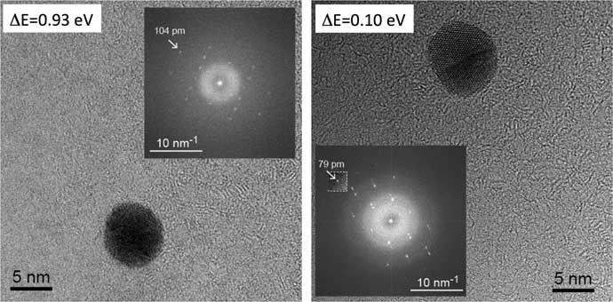
Figure 1 Performance improvement with monochromator on FEI TITAN3 operated at 80 kV. The images are taken from a thin amorphous Ge film with gold particles. The insets show the diffractograms corresponding to the images. The energy spread of incident electrons 0.9 eV (left) is decreased to 0.1 eV (right) when the monochromator is turned on. Without the monochromator we observe a gold diffraction spot associated with an interplanar distance of 104 pm; whereas we can detect a weak spot equivalent to 79 pm when the monochromator is on. Nevertheless, the diffuse scattering from amorphous Ge film appears in both cases up to about 100 pm (10 nm-1).
In the ideal case, the image intensity can be written as ![]() , where 1 and
, where 1 and ![]() represent the incident wave and the scattered wave, respectively. Here, the second and third terms are linear, and the fourth term is non-linear in terms of the scattered wave
represent the incident wave and the scattered wave, respectively. Here, the second and third terms are linear, and the fourth term is non-linear in terms of the scattered wave ![]() . However, an imaging system always suffers from geometrical and chromatic aberrations. Furthermore, the illumination in a TEM is neither perfectly parallel nor monochromatic. Therefore, the image intensity in the real world is the sum of the ideal image intensity for each incident beam direction at each defocus setting. Such non-ideal illumination leads to partial coherency (some physicists describe this as partial incoherency) in conjunction with geometrical and chromatic aberrations. This partial coherency is commonly studied in Fourier space by taking the FT of the image intensity.
. However, an imaging system always suffers from geometrical and chromatic aberrations. Furthermore, the illumination in a TEM is neither perfectly parallel nor monochromatic. Therefore, the image intensity in the real world is the sum of the ideal image intensity for each incident beam direction at each defocus setting. Such non-ideal illumination leads to partial coherency (some physicists describe this as partial incoherency) in conjunction with geometrical and chromatic aberrations. This partial coherency is commonly studied in Fourier space by taking the FT of the image intensity.
Diffractogram (2D FT) analysis
A diffractogram is a power spectrum (squared modulus of a 2D FT) of a single TEM image and has been used to characterize an imaging system. The FT of the-real-world image intensity may be written using the (2D) transmission-cross-coefficient (TCC) T 2 ( k 1 , k 2 ; z), which describes the contribution from two spatial sample frequencies k 1 and k 2 to the image frequency g = k 1 - k 2 due to partial coherency at a defocus z (please consult [Reference Ishizuka5] for details). For a perfectly coherent imaging system, T 2 ( k 1 , k 2 ; z) = 1 for all spatial frequencies and defocus.
For tilted-beam illumination the FT of image intensity may be written by using the TCC where
k
1
or
k
2
is set to the tilted incident-beam direction ![]() :
:
 $$I\left( {{\mib{g}} \,\semi-colon\,z,{\mib \tau } } \right){\equals}{\mib \delta } \left( {\mib{g}} \right){\plus}\Phi \left( {\mib{g}} \right)T_{2} \left( {{\mib{g}} {\plus}{\mib \tau } ,{\mib \tau } \,\semi-colon\,z} \right){\plus}\Phi ^{{\asterisk}} \left( {{\minus}{\mib{g}} )T_{2} } \right.\left( {{\mib{g}} {\minus}{\mib \tau } ,{\minus}{\mib \tau } \,\semi-colon\,z} \right){\plus}non{\minus}linear{\minus}term$$
where Φ(g) is a FT of the scattered wave and the second and third terms correspond to the linear terms of the image formation. The TCC may be written by
 $$T_{2} \left( {{\mib{g}} {\plus}{\mib{\tau }} ,{\mib{\tau }} \,\semi-colon\,z} \right)\proptoE_{t} \left( {{\mib{g}} {\plus}{\mib{\tau }} ,{\mib{\tau }} } \right)E_{s} \left( {{\mib{g}} {\plus}{\mib{\tau }} ,{\mib{\tau }} \,\semi-colon\,z} \right){\times}exp\left\{ {{\minus}2{\mib{\pi }} i\left[ {{\mib{\chi }} \left( {{\mib{g}} {\plus}{\mib{\tau }} \,\semi-colon\,z} \right){\minus}{\mib{\chi }} \left( {{\mib{\tau }} \,\semi-colon\,z} \right)^{2} } \right]} \right\}$$
where ![]() is the wave aberration, and E
t
and E
s
are the temporal and spatial envelopes that describe the reduction in contribution to the image formation due to chromatic and geometrical aberrations, respectively. The spatial envelope E
s
could be ignored for a Cs-corrected high-performance microscope since the spatial envelope depends on the gradient of the wave aberration (that is, geometrical aberration). Therefore, the temporal envelope becomes more important than ever for a Cs-corrected microscope.
is the wave aberration, and E
t
and E
s
are the temporal and spatial envelopes that describe the reduction in contribution to the image formation due to chromatic and geometrical aberrations, respectively. The spatial envelope E
s
could be ignored for a Cs-corrected high-performance microscope since the spatial envelope depends on the gradient of the wave aberration (that is, geometrical aberration). Therefore, the temporal envelope becomes more important than ever for a Cs-corrected microscope.
The temporal envelope for a Gaussian defocus spread with the half-width ∆ may be written as:
 $$E_{t} \left( {{\mib{g}} \,\pm\,{\mib{\tau }} ,\,\pm\,{\mib{\tau }} } \right){\equals}\exp \left\{ {{\minus}\left( {{\mib{\pi }} \Delta } \right)^{2} \left( {{{\mib{\lambda }} \mathord{\left/ {\vphantom {{\mib{\lambda }} 2}} \right. \kern-\nulldelimiterspace} 2}} \right)^{2} \left( {\left| {{\mib{g}} \,\pm\,{\mib{\tau }} } \right|^{2} {\minus}\left| {\mib \tau } \right|^{2} } \right)^{2} } \right\}$$
The defocus spread ∆ for a chromatic aberration coefficient C
C
will be determined by the energy spread of the emitted electrons ∆E, the instability in the high-voltage supply ∆V, and the instability in the objective lens current $\Delta I\,\colon\,\Delta {\equals}C_{C} \sqrt {\left( {{{\Delta E} \mathord{\left/ {\vphantom {{\Delta E} V}} \right. \kern-\nulldelimiterspace} V}} \right)^{2} {\plus}\left( {{{\Delta V} \mathord{\left/ {\vphantom {{\Delta V} V}} \right. \kern-\nulldelimiterspace} V}} \right)^{2} {\plus}4\left( {{{\Delta I} \mathord{\left/ {\vphantom {{\Delta I} I}} \right. \kern-\nulldelimiterspace} I}} \right)^{2} } $
, where V is the mean high-voltage and I is the mean objective lens current. This temporal envelope becomes a familiar expression:
$\Delta I\,\colon\,\Delta {\equals}C_{C} \sqrt {\left( {{{\Delta E} \mathord{\left/ {\vphantom {{\Delta E} V}} \right. \kern-\nulldelimiterspace} V}} \right)^{2} {\plus}\left( {{{\Delta V} \mathord{\left/ {\vphantom {{\Delta V} V}} \right. \kern-\nulldelimiterspace} V}} \right)^{2} {\plus}4\left( {{{\Delta I} \mathord{\left/ {\vphantom {{\Delta I} I}} \right. \kern-\nulldelimiterspace} I}} \right)^{2} } $
, where V is the mean high-voltage and I is the mean objective lens current. This temporal envelope becomes a familiar expression: ![]() for normal illumination
for normal illumination ![]() , which says the contribution will decay with the forth power of spatial frequency. In the case of the tilted-beam illumination, the temporal envelope has no attenuation where
, which says the contribution will decay with the forth power of spatial frequency. In the case of the tilted-beam illumination, the temporal envelope has no attenuation where ![]() , which defines the circle of radius
, which defines the circle of radius ![]() located at
located at ![]() . Since there is no attenuation on this circle due to chromatic aberration, we call it an achromatic circle. Figure 2 shows simulated temporal envelopes E
t
assuming beam-tilt angles of 1, 3, and 5 degrees for 80 kV. Here, we suppose two defocus spreads ∆ of 5.0 nm and 0.5 nm for (a) and (b), respectively, where the square box in (b) corresponds to the whole area of (a). The circle (or the arc) in each figure indicates the position of the achromatic circle. The temporal envelope is sharp for a large beam tilt. However, it becomes broad for a small defocus spread as shown in (b).
. Since there is no attenuation on this circle due to chromatic aberration, we call it an achromatic circle. Figure 2 shows simulated temporal envelopes E
t
assuming beam-tilt angles of 1, 3, and 5 degrees for 80 kV. Here, we suppose two defocus spreads ∆ of 5.0 nm and 0.5 nm for (a) and (b), respectively, where the square box in (b) corresponds to the whole area of (a). The circle (or the arc) in each figure indicates the position of the achromatic circle. The temporal envelope is sharp for a large beam tilt. However, it becomes broad for a small defocus spread as shown in (b).
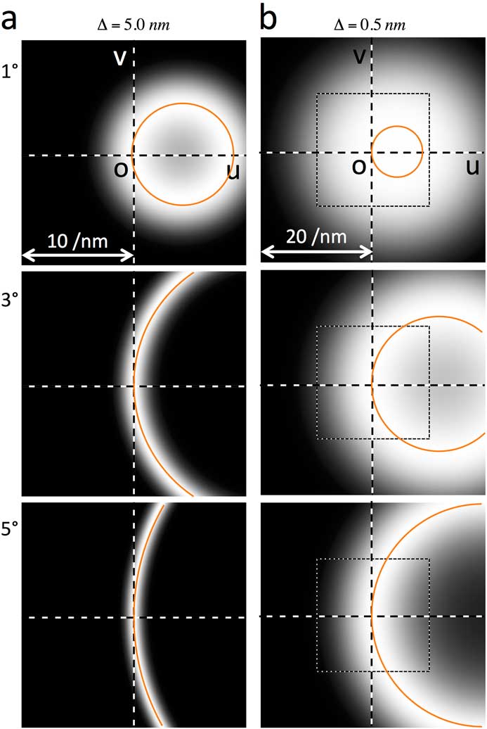
Figure 2 Simulated temporal envelope of tilted-beam diffractograms for 80 kV with a defocus spread of (a) 5.0 nm and (b) 0.5 nm. The beam-tilt angles from top to bottom are 1, 3, and 5 degrees, respectively. The scale bars of (a) and (b) are 10 and 20 nm-1, respectively, and the square box in (b) corresponds to the whole area of (a). The circle, or the arc, of each figure shows the achromatic circle, where there is no attenuation of the temporal envelope. The temporal envelope becomes narrow for a large beam tilt, and it becomes broad for a small defocus spread.
Now, we consider the diffractogram D, which is the squared modulus of 2D FT:
 $$D\left( {{\mib{g}} \,\semi-colon\,z,{\mib \tau } } \right){\equals}M\left( {\mib{g}} \right)\left| {I\left( {{\mib{g}} \,\semi-colon\,z,{\mib \tau } } \right)} \right|^{2} \,\approx\,M\left( {\mib{g}} \right)\left| {\Phi _{s} \left( {\mib{g}} \right)} \right|^{2} \left| {T_{2} \left( {{\mib{g}} {\plus}{\mib \tau } ,{\mib \tau } ,z} \right){\minus}T_{2} \left( {{\mib \tau } ,{\mib \tau } {\minus}{\mib{g}} ,z} \right)} \right|^{2} $$
where we neglect the non-linear term in Eq. (1) and include the rotationally symmetric dumping function M, such as the modulation transfer function (MTF) of the recording system. Here, we assume the relation ![]() (that is, kinematical scattering) for the scattered wave, which restricts applicability of the diffractogram analysis only to a weak scattering sample. In the case of a Cs-corrected microscope, since the information limit is mainly determined by the temporal envelope as described above, the diffractogram may be approximated by
(that is, kinematical scattering) for the scattered wave, which restricts applicability of the diffractogram analysis only to a weak scattering sample. In the case of a Cs-corrected microscope, since the information limit is mainly determined by the temporal envelope as described above, the diffractogram may be approximated by
 $$D\left( {{\mib{g}} \,\semi-colon\,z,{\mib \tau } } \right)\,\approx\,M\left( {\mib{g}} \right)\left| {\Phi _{s} \left( {\mib{g}} \right)} \right|^{2} \left( {E_{t}^{2} \left( {\plus} \right){\plus}E_{t}^{2} \left( {\minus} \right){\minus}2E_{t} \left( {\plus} \right)E_{t} \left( {\minus} \right)\cos \left( {{\minus}2{\mib \pi } i\left[ {{\mib \chi } \left( {\plus} \right){\plus}{\mib \chi } \left( {\minus} \right){\minus}2{\mib \chi } } \right]} \right)} \right)$$
where the last term describes interference between two linear terms. In this equation Et(±) and ![]() respectively denote the temporal envelope and the wave aberration function for the beam-tilt directions
respectively denote the temporal envelope and the wave aberration function for the beam-tilt directions ![]() or
or ![]() . The diffractogram for the normal illumination becomes
. The diffractogram for the normal illumination becomes ![]() , where sinusoidal oscillations are known as Thon’s rings [Reference Thon6]. We note that an absolute measurement of the temporal envelope from the normal-beam diffractogram is difficult since it requires information on the rotationally symmetric dumping factors such as the MTF, M(
g
), and the scattering behavior of the sample,
, where sinusoidal oscillations are known as Thon’s rings [Reference Thon6]. We note that an absolute measurement of the temporal envelope from the normal-beam diffractogram is difficult since it requires information on the rotationally symmetric dumping factors such as the MTF, M(
g
), and the scattering behavior of the sample, ![]() .
.
In the case of the tilted-beam diffractogram, we can measure the rotationally symmetric factors using the fact that the temporal envelope has no attenuation on the achromatic circle. In addition, oscillations (Thon’s rings) of the diffractogram may be washed out by applying a low-pass filter [Reference Barthel and Thust1] or may be ignored by considering the envelope of the oscillations [Reference Haider2]. Nevertheless, even such tilted-beam diffractogram analysis may become difficult for evaluating a Cs-corrected microscope with a Cc-corrector or a monocromator since the temporal envelope becomes broad for a small defocus spread. As noted before an analysis of the temporal envelope at high-angle requires a strong scattering sample, which will inevitability introduce the strong non-linear term in the diffractogram. However, diffractogram analysis cannot be applied to such a sample since it does not distinguish between linear and non-linear contributions, contrary to the 3D FT analysis discussed in the next section.
3D FT analysis
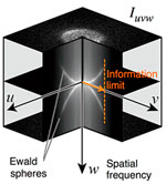
Figure 3 schematically shows the 3D FT analysis in the case of the normal illumination. Figure 3a is a stack of through-focus images, I xyz , as a function of the defocus z, while Figure 3c is the 3D FT of the image stack, I uvw , which shows two spheres called Ewald spheres. The figure in the middle (Figure 3b) shows a stack of the diffractograms (2D FT), I uvz , of each image intensity. We note that the information limit can be roughly estimated from an observable range of the Ewald spheres as indicated in Figure 3c. However, the intensity on the Ewald sphere is affected also by the rotationally symmetric attenuation factors as in the case of the diffractogram. Therefore, a quantitative evaluation of the temporal envelope requires a 3D FT analysis of tilted-beam through-focus images.
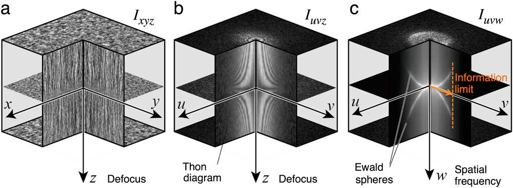
Figure 3 Schematics showing the 3D FT analysis in the case of the normal illumination. (a) I xyz : stack of acquired through-focus TEM images. (b) I uvz : stack of the 2D FT (diffractogram) of each image. (c) I uvw : 3D FT of the image stack. The 3D FT shows two Ewald spheres that attach at the origin and are rotationally symmetric around the w-axis. The information limit can be estimated from the fading of the 3D FT intensity on the Ewald spheres as indicated by a vertical broken line in (c). In the case of a tilted-beam illumination, the two Ewald spheres slant as shown in Figures 4 and 5.
In practice a 3D FT is calculated by taking a 3D FT of the image stack in a single step. Here, however, we evaluate a 3D FT in two steps, namely by taking a 2D FT of each image of the image stack to give I
uvz
and then taking a 1D FT of I
uvz
along z-axis. This will make clear the relation between the 2D FT (diffractogram) and the 3D FT. We note that the 2D FT of a tilted-beam image (Eq. 1) depends on z only through the 2D TCC (Eq. 2), which in turn depends on the defocus term of the wave aberration function ![]() . We have neglected the spatial envelope
. We have neglected the spatial envelope ![]() for simplicity. For a complete analysis, please see [Reference Ishizuka and Kimoto7]. Thus, the 3D FT of the image stack may be written by replacing T
2 in Eq. (1) with the 3D TCC T
3, which is a FT of the 2D TCC along the z-direction:
for simplicity. For a complete analysis, please see [Reference Ishizuka and Kimoto7]. Thus, the 3D FT of the image stack may be written by replacing T
2 in Eq. (1) with the 3D TCC T
3, which is a FT of the 2D TCC along the z-direction:
 $$T_{3} \left( {{\mib{g}} \,\pm\,{\mib \tau } ,{\mib \tau } ,w} \right)\proptoE_{t} \left( {{\mib{g}} \,\pm\,{\mib \tau } ,\,\pm\,{\mib \tau } } \right) \cdot E_{{Ewald}} \left( {{\mib{g}} \,\pm\,{\mib \tau } ,\,\pm\,{\mib \tau } _{2} ,w} \right)$$
 $$E_{{Ewald}} \left( {{\mib{g}} \,\pm\,{\mib \tau } ,{\mib \tau } ,w} \right){\equals}{1 \mathord{\left/ {\vphantom {1 {\sqrt {\mib \pi } q_{0} {\mib \lambda } g}}} \right. \kern-\nulldelimiterspace} {\sqrt {\mib \pi } q_{0} {\mib \lambda } g}}exp\left[ {{\minus}{{\left( {w{\minus}w_{E}^{\,\pm\,} \left( {\mib{g}} \right)} \right)^{2} } \mathord{\left/ {\vphantom {{\left( {w{\minus}w_{E}^{\,\pm\,} \left( {\mib{g}} \right)} \right)^{2} } {\left( {q_{0} {\mib \lambda } g} \right)^{2} }}} \right. \kern-\nulldelimiterspace} {\left( {q_{0} {\mib \lambda } g} \right)^{2} }}} \right]$$
Here, we assume the distribution of incident beam directions is a Gaussian with half-width of q
0. We can verify that the parameter w
E
(
g
) corresponds to the distance along the w-axis from the uv-plane to the Ewald sphere: ![]() [Reference Ishizuka and Kimoto7]. The function E
Ewald
may be called the Ewald sphere envelope and takes the form
[Reference Ishizuka and Kimoto7]. The function E
Ewald
may be called the Ewald sphere envelope and takes the form ![]() for all the spatial frequencies g on the Ewald sphere (w = w
E). In the limit of perfectly parallel illumination, the Ewald-sphere envelope becomes a delta function and takes the value of unity only on the Ewald sphere.
for all the spatial frequencies g on the Ewald sphere (w = w
E). In the limit of perfectly parallel illumination, the Ewald-sphere envelope becomes a delta function and takes the value of unity only on the Ewald sphere.
Figure 4a shows an example of the simulated Ewald-sphere envelopes, where the beam tilt is 2 degrees and the beam convergence angle is 3.0 mrad. We note that the intersection of the Ewald-sphere envelope with the uv-plane coincides with the achromatic circle. Other simulated Ewald-sphere envelopes with different beam-tilt and convergence angles are shown in Figure 4b. The Ewald-sphere envelope, especially the uw-section, is too thin to be drawn for a small beam convergence. It is important to note that the Ewald-sphere envelope is sharp even for a rather large convergence angle of 3.0 mrad and does not depend on the defocus-spread contrary to the temporal envelope. Therefore, we can measure the temporal envelope on the sharp Ewald-sphere envelope, even when the temporal envelope becomes broad for the case of a small defocus spread.
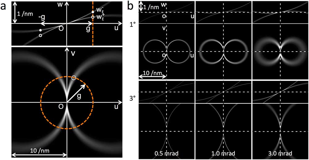
Figure 4 Simulated Ewald-sphere envelopes for 80 kV electrons. (a) The top and bottom panes show uw- and uv-sections of the 3D FT, respectively. Here, the beam tilt is 2 degrees, and the beam convergence is 3 mrad. The uw-section shows two Ewald-sphere envelopes that are separate from each other except in the region close to the origin. (b) Ewald-sphere envelopes for beam-tilt angles of 1 and 3 degrees (top to bottom) and beam convergences of 0.5, 1.0, and 3.0 mrad (left to right). The Ewald-sphere envelope is sharp even for a rather large convergence angle of 3.0 mrad. Note that the Ewald-sphere envelope, especially the uw-section, is too thin to be drawn for a small beam convergence. The location of the Ewald sphere does not move by changing the beam convergence angle.
It is noted further that the two linear terms of Eq. (1) are separate from each other on Ewald-sphere envelopes, except in the region close to the Fourier space origin as shown in Figure 4. Therefore, we can separately analyze the two linear image contributions independently. This means that we do not need to assume the relation ![]() (kinematical scattering) as required by diffractogram analysis. Thus, we can use a thick sample or a sample made from strong scattering elements, which will lead to dynamical scattering. This is essential if we need to directly observe the linear image transfer down to a few tens of pm.
(kinematical scattering) as required by diffractogram analysis. Thus, we can use a thick sample or a sample made from strong scattering elements, which will lead to dynamical scattering. This is essential if we need to directly observe the linear image transfer down to a few tens of pm.
Applications
We use a TEM (FEI, TITAN3) equipped with a monochromator, a Cs-corrector for image forming (CEOS, CETCOR), a CCD camera (Gatan Inc., UltraScan), and an energy filter (Gatan Inc., Quantum) operated at acceleration voltage of 80 kV. We have acquired a set of through-focus images from a thick amorphous carbon film (36 nm) with a beam tilt of 36 mrad [Reference Kimoto4]. Here, a series of 129-images was acquired with a small defocus step of 1.37 nm around exact focus. Thus, the total focus range was 176.7 nm. The image size was 1024 × 1024 pixels with 2 × 2 binning, and the pixel size on the specimen was 26.5 pm. The specimen drift of the through-focus images was corrected using cross-correlation between neighbor images. Figures 5a and Figure 5b show respectively the vw- and uv-sections of the 3D FT of the stacked images of 512 × 512 pixels extracted from the drift-corrected images. Here, the arcs are the intersections of the product of the temporal envelope E
t
and the Ewald-sphere envelope E
Ewald
(Eq. 4). From the uw-section, we measure the product ![]() for a spatial frequency
g
(see the to p pane of Figure 4a or Figure 5a). From the uv-section we measure another product on the circle of radius of g (see the bottom pane of Figure 4a or Figure 5b), which gives
for a spatial frequency
g
(see the to p pane of Figure 4a or Figure 5a). From the uv-section we measure another product on the circle of radius of g (see the bottom pane of Figure 4a or Figure 5b), which gives ![]() , since there is no attenuation on the achromatic circle
, since there is no attenuation on the achromatic circle ![]() . When we note that the Ewald-sphere envelope for the same spatial frequency takes the same value (namely,
. When we note that the Ewald-sphere envelope for the same spatial frequency takes the same value (namely, ![]() ), the ratio of the measurement on uw-section to the one on uv-section, H(
g
), will give the temporal envelope:
), the ratio of the measurement on uw-section to the one on uv-section, H(
g
), will give the temporal envelope:
 $$\displaylines{ H\left( {\mib{g}} \right){\equals}{{\left( {\sqrt {M\left( g \right)} \left| {\Phi \left( g \right)} \right|E_{t}^{{uw}} \left( g \right)E_{{Ewald}}^{{uw}} \left( g \right)} \right)} \mathord{\left/ {\vphantom {{\left( {\sqrt {M\left( g \right)} \left| {\Phi \left( g \right)} \right|E_{t}^{{uw}} \left( g \right)E_{{Ewald}}^{{uw}} \left( g \right)} \right)} {\left( {\sqrt {M\left( g \right)} \left| {\Phi \left( g \right)} \right|E_{{Ewald}}^{{uv}} \left( g \right)} \right)}}} \right. \kern-\nulldelimiterspace} {\left( {\sqrt {M\left( g \right)} \left| {\Phi \left( g \right)} \right|E_{{Ewald}}^{{uv}} \left( g \right)} \right)}} \cr {\equals}E_{t}^{{uw}} \left( g \right){\equals}exp\left\{ {{\minus}\left( {{\mib \pi } \Delta } \right)^{2} \left( {{{\mib \lambda } \mathord{\left/ {\vphantom {{\mib \lambda } 2}} \right. \kern-\nulldelimiterspace} 2}} \right)^{2} \left( {\left| {{\mib{g}} \,\pm\,{\mib \tau } } \right|^{2} {\minus}\left| {\mib \tau } \right|^{2} } \right)^{2} } \right\} \cr {\equals}exp\left\{ {{\minus}\left( {{\mib \pi } \Delta } \right)^{2} w_{E}^{2} \left( {\mib{g}} \right)} \right\} \cr} $$
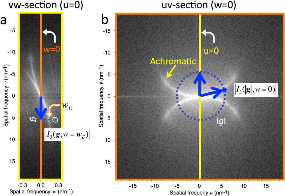
Figure 5 The 3D FTs of experimental though-focus images. (a) and (b) show the uw- and uv-sections of the 3D FT, respectively. Here, the sample is a thick amorphous carbon (36 nm). A series of 129 images was acquired using FEI, TITAN3 equipped with a monochromator operated at an acceleration voltage of 80 kV. After the specimen drift correction, the region of 512 × 512 pixels is extracted for a 3D FT. The white arcs are the sections of two Ewald spheres on the corresponding planes. The Ewald sphere on the uv-plane coincides with achromatic circle. The intensity of the 3D FT is measured on each section for the spatial frequency g as illustrated. The ratio of these measurements is used to plot each point in Figure 6.
The last equation is obtained by noting ![]() . This means that the ratio H(
g
) is a simple function of w
E
, which is the distance to the Ewald sphere for the spatial frequency
g
. Figure 6 plots some H values measured at several values of w
E
. In this case, the experimental values decrease to 1/e2 (H(
g
) = 13.5%) at w
E
of 0.26 nm.-1 Then, from the relation
. This means that the ratio H(
g
) is a simple function of w
E
, which is the distance to the Ewald sphere for the spatial frequency
g
. Figure 6 plots some H values measured at several values of w
E
. In this case, the experimental values decrease to 1/e2 (H(
g
) = 13.5%) at w
E
of 0.26 nm.-1 Then, from the relation ![]() we obtain the defocus spread ∆ of 1.73 nm. Finally, with this defocus spread, the temporal envelope for normal illumination, exp
we obtain the defocus spread ∆ of 1.73 nm. Finally, with this defocus spread, the temporal envelope for normal illumination, exp ![]() , gives the spatial frequency of 11.2 nm-1 using the 1/e2 (13.5%) criterion [Reference Spence8]. This spatial frequency corresponds to a linear information limit of 90 pm (Table 1).
, gives the spatial frequency of 11.2 nm-1 using the 1/e2 (13.5%) criterion [Reference Spence8]. This spatial frequency corresponds to a linear information limit of 90 pm (Table 1).
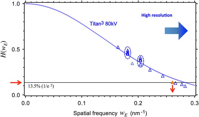
Figure 6 Information limit measured by 3D FT analysis of our FEI TITAN3 operated at 80 kV when the monochromator is ON. Each point on the figure is a ratio of two measurements of the Ewald envelopes for the spatial frequency g on the vw- and uv-sections. The horizontal axis corresponds to w E , which is the distance to the Ewald sphere for the spatial frequency g. Here, the ratio H decreases to 1/e2 (13.5%) at w E of 0.26 nm-1, which gives a defocus spread ∆ of 1.73 nm (see text).
Table 1 Information limit (highest spatial frequency) at 80 kV estimated using various criteria.

Note: The linear information limit is determined by the 3D FT analysis using w E = 0.26 nm-1, while the nominal information limit is estimated by the energy spread (FWHM) of 0.1 eV of incident electrons measured by EELS. The highest-order diffraction spot was observed from a gold particle.
Discussion
The linear information limit of our monochromated TITAN3 is evaluated to be 90 pm (11.2 nm-1) when the monochromator is on. However, we have shown that the image taken with the monochromator gives a faint spot at 79 pm from a gold particle (Figure 1b). From the 3D FT analysis, we can conclude that the faint spot should result from the non-linear effect. Thus, the information limit actually is not improved down to 79 pm by using the monochromator. We may note that in most of the cases a faint spot in the FT of a HRTEM image does not indicate a linear spatial resolution of a microscope, although such information exists in the image intensity. This is because the spatial frequency up to twice the image wave frequency is recorded in the image intensity. Surprisingly, the diffuse scattering from an amorphous Ge film appears only up to about 100 pm (see the right pane of Figure 1), and thus Young’s fringe methods gives a resolution of 100 pm, which is worse than the estimate from the 3D FT analysis. This indicates that the rotationally symmetric attenuation factors surpass the normal-illumination temporal envelope at high spatial frequency when the monochromator is on.
An information limit is determined by the defocus spread that depends on three terms: ∆E (the energy spread of emitted electrons), ∆V (the instability in the high-voltage) and ∆I (the instability of lens current). Among them the instability of lens current does not change the velocity of electrons, although it slightly changes the shape of electron beam. Therefore, we can measure the sum of ∆E and ∆V by using the electron energy filter that disperses the electrons by their velocity (kinetic energy), and thus estimate a nominal information limit due to the energy spread of incident electrons. We have measured the energy spread (FWHM) of incident electrons using the energy filter (Gatan, Inc., Quantum) as 0.1eV when the monochromator is on. The energy spread of 0.1eV (FWHM) of incident electrons gives a defocus change ∆
FWHM
of 1.9 nm [Reference Kimoto3] and a defocus spread ∆ is estimated to be 1.14 nm from the relation ![]() . Thus, we obtain the nominal information limit of 73 pm (Table 1), which is much better than the information limit of 90 pm measured by the 3D FT analysis. This indicates that other sources of chromatic aberration, namely the objective lens current fluctuation and/or instability of the Cs-corrector, cannot be ignored when the energy spread is reduced to 0.1 eV by using the monochromator. In other words, the objective lens and/or the Cs-corrector should be stabilized further in order to enjoy the full benefit of the monochromator. Thus, it becomes apparent that the 3D FT analysis is an indispensable tool to evaluate a high-performance microscope. This is the answer to the question posed in the title of this article.
. Thus, we obtain the nominal information limit of 73 pm (Table 1), which is much better than the information limit of 90 pm measured by the 3D FT analysis. This indicates that other sources of chromatic aberration, namely the objective lens current fluctuation and/or instability of the Cs-corrector, cannot be ignored when the energy spread is reduced to 0.1 eV by using the monochromator. In other words, the objective lens and/or the Cs-corrector should be stabilized further in order to enjoy the full benefit of the monochromator. Thus, it becomes apparent that the 3D FT analysis is an indispensable tool to evaluate a high-performance microscope. This is the answer to the question posed in the title of this article.
Next, we would like to discuss the practical aspects of the 3D FT. Whereas the 3D FT analysis looks to be rather involved compared with the 2D FT analysis (diffractogram), these days we can easily acquire through-focus images automatically using a homemade script or a free plug-in for DigitalMicrograph [9]. Furthermore, we can perform a FT of a 3D data set using a built-in command of DigitalMicrograph or a versatile free plug-in [10]. When your microscope is stable enough, you can take a 3D FT just after image acquisition. If the image drift is constant during the experiment, you will obtain a 3D FT that is simply distorted by image drift. When the image drift is time-dependent during a focal-series acquisition, however, you have to remove such image drift using the cross-correlation between the images.
Other aspects of the 3D FT analysis are the defocus step and the number of images in the through-focus series. In a 2D FT of an image, the pixel size determines the highest special frequency of the FT, and the image size (number of pixels × pixel size) determines the finest step of the 2D FT. Analogously, the defocus step determines the highest spatial frequency of the 3D FT along the w-axis, and the defocus range (number of images × defocus step) determines the finest step along the w-axis. Therefore, if we use the same defocus step, we can calculate the same Fourier space with a coarse step as shown in Figure 7. Here, all the pixels (1018 × 1018) after the drift correction are used to improve the signal-to-noise ratio. The 3D FT calculated using 64 images shown in Figure 7b does not show significant degradation from the FT calculated using all 129 images in Figure 7a. Even the 3D FT calculated using 32 images shown in Figure 7c gives an approximate estimation of the highest w E , and thus the defocus spread.
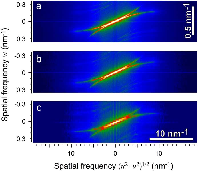
Figure 7 The 3D FTs calculated from a smaller number of though-focus images. Plots (a) to (c) shown in pseudo-color the 3D FTs are calculated from 129, 64, and 32 images, respectively. Since the focal step does not change, we can calculate the same range of Fourier space along the w-direction, although the resolution becomes poor. Note that the FT in (b) does not show significant degradation from the FT in (a). Even from the FT in (c) we can estimate the highest w E and thus the defocus spread.
Finally, we would like to discuss the implication of 3D FT analysis on an electron microscope with a Cc-corrector. The Cc-corrector reduces an apparent chromatic aberration due to different velocity (kinetic energy) of incident electrons by introducing a negative chromatic aberration. Namely, the Cc corrector creates a fine probe by changing the beam path but does not modify the velocity of electrons. Importantly, the Cc-corrector does not reduce chromatic aberration caused by the current fluctuation of the objective lens. Furthermore, a Cc-corrector will increase total chromatic aberration due to its own current fluctuations. Thus, it is advisable to preform a 3D FT analysis to evaluate the total defocus spread of Cs-corrected microscopes with a Cc-corrector.
Conclusions
We have compared 3D FT analysis with diffractogram analysis (2D FT analysis) for evaluating the performance of a high-resolution TEM. The significant difference of the 3D FT analysis from the diffractogram analysis is its ability to separately analyze two linear image contributions on two spheres in Fourier space that we call Ewald spheres. Then, we don’t need to assume a weak phase object approximation, and we can use a thick sample or a sample made from strong scattering elements. In short, we need the 3D FT analysis to directly observe the linear image transfer down to a few tens of pm that will be attained by a Cs-corrected microscope equipped with a Cc-corrector or a monochromator.
The tilted-beam 3D FT analysis of our microscope gives the information limit of 90 pm at 80 kV when the monochromator is on, while the nominal information limit of 73 pm is obtained from an energy spread of incident electrons. This suggests that other instabilities in the lens currents and/or the Cs-corrector becomes dominant when the monochromator is used at 80 kV, and that performance improvement may be obtained by reducing those instabilities.
The 3D FT analysis will give an unbiased means to evaluate the performance of a TEM. Therefore, we strongly recommend that the owners of a Cs-corrected electron microscope at first perform 3D FT analyses of normal-incidence images and roughly evaluate the highest spatial frequency contributing linearly to image formation. If you are really interested in evaluating your microscope more accurately, then try an elaborate tilted-beam 3D FT analysis that can exclude the effects from rotationally symmetric attenuation factors.
Acknowledgements
The authors are heavily indebted to Prof. C. Lyman, the editor of Microscopy Today, who has made appropriate comments and encouraged us to make the article more readable for a wider audience. This study was partly supported by the JST Research Acceleration Program and the Nano Platform Program of MEXT, Japan.


