Introduction
For more than 150 years light microscopy, employing glass lenses to focus light and produce the phenomenon of magnification, has allowed the observation of minuscule entities not visible to the unaided eye. Today there are many types of light microscopes, but here we discuss two of the most common: (1) digital microscopes employing electronic image sensors, but no eyepieces, where the image is displayed on an electronic monitor, and (2) microscopes for direct visual observation which have eyepieces and a digital camera, allowing it to be used in a similar manner to a digital microscope.
A feature of interest for any microscope is magnification. Image magnification is the apparent size of an object at a scale larger (or smaller) than its actual size. Magnification serves a useful purpose only when the resolution of the microscope makes it possible to see more details of an object in the image than when observing the object with the unaided eye. Until recently, magnification has been well defined when viewing an image of a sample through the eyepieces of a microscope. For this case, rigorous international standards have been documented [1–8]. Many of these standards also apply to digital microscopy, but strict definitions and standards for magnification achieved by a digital microscope, where the image is viewed on an electronic monitor, have been developed only in the last few years [9].
In research publications and presentations, images must include a calibrated scale bar or a statement of the width of the field of view, typically in nm or µm. However, when viewing images in real-time on monitors of various sizes, indications of scale may not be shown, and the instantaneous magnification of an image may not be known. Moreover, there is typically a lower and higher limit of magnification which define the range of useful magnification. Digital microscopes, as well as microscopes for visual observation equipped with digital cameras, allow the rapid acquisition of high-quality images. These instruments are applied in various scientific and engineering fields.
The goal of this article is to provide digital microscopy users with helpful guidelines so they can determine the range of useful magnification when making observations and measurements. The specific parameter values given here are for instruments from Leica Microsystems, but the principles described are quite general for all light microscopes employing digital image acquisition and display.
Magnification
What exactly is magnification? Magnification is the ratio of the size of an object in an image produced by an optical system to the actual size of the object itself. Thus, lateral magnification, M DIS , can be defined as:
 $$M_{{DIS}} {\rm {\equals}}{{{\rm dimension}\,{\rm of}\,{\rm an}\,{\rm object}\,{\rm in}\,{\rm the}\,{\rm image}} \over {{\rm true }\,{\rm dimension}\,{\rm of}\,{\rm the}\,{\rm object}}}$$
Of course, the upper limit of visual magnification depends on the maximum resolving power of the microscope system. When the magnification is pushed above the useful range, no additional details about the sample can be seen. This situation is referred to as empty magnification [10]. Even within the microscope’s resolving power, the practical level of observable detail also depends on the distance between the display of the image and the observer’s eyes.
Microscopes with Digital Sensors
Magnification in conventional light microscopes
When observing the image through the eyepieces of a microscope for visual observation, the total magnification is defined as [5, 6]:
 $$M_{{TOT{\rm }VIS}} {\equals}{\rm }M_{O} \cdot{\rm }q{\rm }\cdot{\rm }M_{E} $$
where M TOT VIS is the total lateral magnification observed through the eyepiece, M O is the objective lens magnification, q is the total tube factor (zoom and other tube lenses), and M E is the eyepiece lens magnification. As an example, a microscope with a 40× objective (M O = 40×), total tube factor of 1× (q = 1×), and 10× eyepieces (M E = 10×), then the total magnification (M TOT VIS ) seen via the eyepieces would be: M TOT VIS = 40× · 1× · 10× = 400×.
Magnification at the digital sensor
For the case of a microscope image that is projected onto an electronic sensor, such as that of a digital camera, the magnification for the image formed at the sensor is [5, 6]:
 $$M_{{TOT{\rm }PROJ}} {\equals}M_{O} \cdotq\cdotM_{E} \cdotp\left( {{\rm projection}\,{\rm via}\,{\rm eyepiece}} \right)$$
 $$M_{{TOT{\rm }PROJ}} {\equals}M_{O} q\cdotM_{{PHOT}} \,\left( {{\rm projection}\,{\rm via}\,{\rm tube}} \right)$$
where M TOT PROJ is the (lateral) magnification of the microscope (image projected onto the sensor), p is the projection factor from eyepiece to camera, and M PHOT is the magnification of the photographic projection lens from tube to camera. Standard values for the total tube factor, q, fall between 0.5:1 and 25:1 [1]. Standard values for the photographic projection lens magnification, M PHOT , fall between 0.32:1 and 1.6:1 [1].
Digital microscopes
For digital microscopes, there are no eyepieces, so an image is projected onto and detected by the electronic sensor and displayed on an electronic monitor for observation. The same is also true for a microscope for visual observation equipped with a digital camera when the image is observed via a monitor. Thus, the final total magnification for digital microscopy, M DIS (Equation 1), will always depend on the size of the image on the monitor versus the size on the sensor and can be defined as:
 $$M_{{DIS}} {\equals}M_{{TOT{\rm }PROJ}} \cdot{\rm }pixel\,size\,ratio$$
where M DIS is the total lateral display magnification for an image displayed on a monitor, and the image size ratio is the “enlargement” of the image from the sensor to the electronic monitor display. As an example, if a microscope has a 20× objective (M O = 20×), total tube factor of one (q = 1), a 0.5× photographic projection lens (M PHOT = 0.5×), and a sensor and monitor with an image size ratio of 100:1, then the total display magnification (M DIS ) seen via the image displayed on the monitor would be: M DIS = 20× · 1× · 0.5× · 100 = 1,000×.
For an image size ratio, just one dimension could be used, such as the image width. The size of the image width on the monitor equals the number of monitor pixels in the image width times the pixel size. The same type of argument applies for the image width on the sensor:
The ratio of the monitor to sensor pixel size can be defined as the pixel size ratio:
When the number of monitor and sensor pixels are the same (a 1-to-1 pixel correspondence), then:![]()
As just stated, the pixel size ratio is the ratio of the pixel size of the monitor to that of the sensor:
 $$pixel\,size\,ratio{\rm {\equals} }{{monitor\,pixel\,size } \over {sensor\,pixel\,size }}$$
For Equation 5, it is assumed that the number of pixels across the image on both the sensor and the monitor occur in a 1-to-1 pixel correspondence mode, that is, one monitor pixel displays the signal from a corresponding single sensor pixel, the simplest case scenario. In this display mode, only a portion of the image may be visible on the monitor, depending on the actual total number of pixels across the image, the final magnification, and the difference in the number of pixels between the camera sensor and monitor [11]. Figure 1 shows two examples of modern light microscopes: (a) a conventional stereo microscope with eyepieces, a digital camera, and two sizes of display monitor, and (b) a direct digital microscope with 2 sizes of display monitor, but without eyepieces.
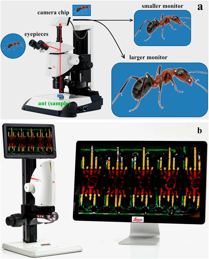
Figure 1 (a) Stereo microscope (M205 C) equipped with a digital camera. The ant sample can be observed via the eyepieces or on an electronic monitor displaying the image from the sensor in the camera. (b) Digital microscope (DMS1000) shown with two different monitor sizes for image display.
Resolution
For optical instruments in general, resolution or resolving power is the ability to see fine details in an image. More specifically, resolving power is the ability to distinguish in an image adjacent points or lines of the object that are closely spaced. Sometimes the terms magnification and resolution are used synonymously, but this is incorrect. Only resolution determines the limit of the smallest object that can be resolved. Magnification denotes the size of the resolved object. In light microscopy, resolution is typically expressed in line pairs per millimeter observed when lines of various separations are used as the object. In other words, at a given level of resolution pairs of black and white lines with equal line thickness and spacing can be distinguished. High magnification without sufficient resolution leads to empty magnification, as mentioned above [10]. Therefore, it is of vital importance to understand the limiting factors for resolution, not just for digital light microscopy, but for all forms of microscopy.
Image Sensor and Display Monitor Combinations
Pixel number and size
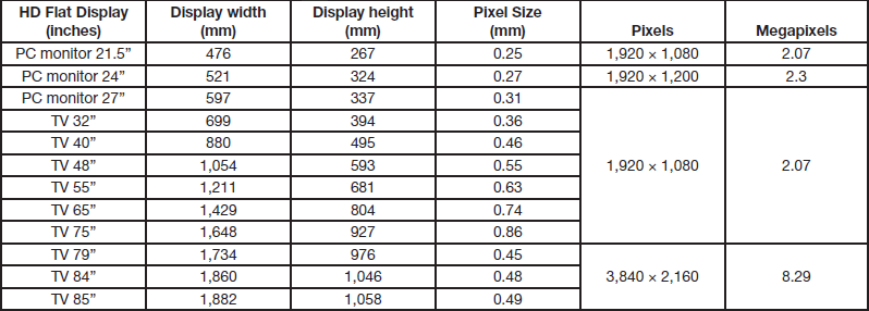
Image sensors used in most microscope digital cameras have a number of pixels typically between 1,600 × 1,200 and 5,472 × 3,648 and a pixel size between 1.5 µm and 6 µm (see examples in Table 1). High-definition (HD) electronic displays, including computer monitors and televisions, typically have minimum pixel numbers of 1,200, 1,080, or 2,160 pixels and pixel sizes between 0.12 and 0.9 mm (see Table 2) [12, 13]. Therefore, monitor pixels are typically 20 to 600 times larger than camera pixels.
Table 1 Specifications of image sensors used in digital cameras and microscopes supplied by Leica Microsystems.
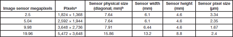
a By convention the sensor width is given first.
b Sensor sizes are sometimes still given in arcane terms that originated in the vacuum tube era, e.g., 1/2.3” means a sensor 6.1 × 4.6 mm. Even then a 1/2.3” sensor from different manufacturers may have slightly different dimensions.
Table 2 Examples of high definition displays including both computer monitors and TVs.

Pixel size ratio
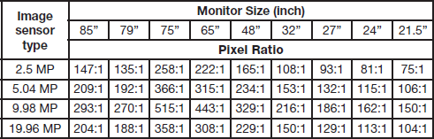
Knowing pixel sizes of image sensors (Table 1) and flat-screen HD monitors (Table 2), values for pixel size ratios can be calculated using Equation 5 (see Table 3).
Table 3 Pixel size ratios (Equation 5) for HD monitors (Table 2) and image sensors used in digital microscopes and cameras supplied by Leica Microsystems (Table 1).
Digital Microscopes and Stereo Microscopes with Digital Cameras
Total magnification
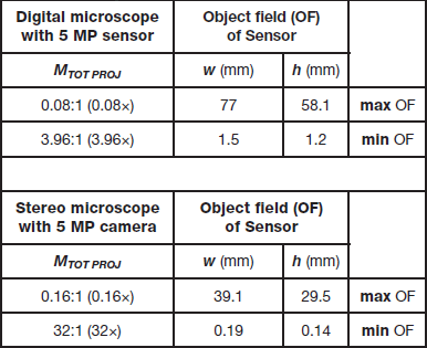
For simplicity, only two examples of digital microscopy are described here: a digital microscope and a stereo microscope equipped with a digital camera installed with a C-mount. It is assumed that in each case an image is displayed, using a 1-to-1 camera-to-monitor pixel correspondence, onto an HD monitor where sizes range from 21.5” (diagonal dimension 21.5 inches [54.6 cm]) to 75” (diagonal dimension 74.5 inches [189 cm]). Both microscopes use a 5 MP image sensor. Table 4 shows examples of total magnification values (expressed as image size divided by object size) obtainable with the digital microscope or stereo microscope with digital camera.
Table 4 Total magnification data, MTOT VIS and MDIS (Equations 2 and 4b), for a digital microscope with 5 MP image sensor (DMS1000) and a stereo microscope (M205 A) equipped with a 5 MP digital camera. The possible range of magnification values, minimum to maximum, for the discussed HD monitor sizes (Table 2) and pixel ratios (Table 3) are shown.
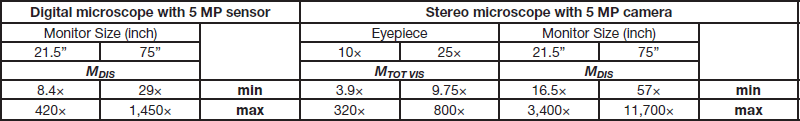
For the digital microscope, the magnification range for the objective lens is 0.32× to 2×, and the tube factor (q) including the photographic projection lens has a maximum to minimum magnification range of 8:1 (ratio of max to min tube factor magnification). For the stereo microscope with camera, the magnification range for the objective is 0.5× to 2×, for the zoom from 0.78× to 16×, for the eyepieces 10× to 25×, and for the C-mount lens from 0.4× to 1×. Using Equations 2 and 4b, example calculations for the minimum and maximum magnification values (M TOT VIS and M DIS in table 4) achievable with the stereo microscope having a 5 MP camera sensor can be shown. The stereo microscope has a min and max objective magnification of M O = 0.5× or 2×, a min and max zoom factor of q = 0.78× or 16×, a min and max C-mount magnification of M PHOT = 0.4× or 1×, and a min and max eyepiece magnification of M E = 10× or 25×. Then the minimum and maximum total magnification (M TOT VIS ) seen via the eyepieces would be:
 $$\eqalignno{ & {\rm Minimum\,\colon\,}\quad M_{{TOT{\rm }VIS}} {\equals}{\rm }0.5{\times}\cdot{\rm }0.78{\times}\cdot{\rm }10{\times}{\equals}{\rm }3.9{\times} \cr & {\rm Maximum}\,\colon\,\quad M_{{TOT{\rm }VIS}} {\equals}{\rm }2{\times}\cdot{\rm }16{\times}\cdot{\rm }25{\times}{\equals}{\rm }800{\times}. \cr} $$
Also, the total display magnification (M DIS ) seen via an image displayed on a 21.5” or 75” monitor (table 2) with a pixel size ratio of 106:1 and 366:1 (table 3) would be:
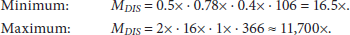 $$\eqalignno{ & {\rm Minimum}\,\colon\, \quad M_{{DIS}} {\equals}{\rm }0.5{\times}\cdot{\rm }0.78{\times}\cdot{\rm }0.4{\times}\cdot{\rm }106{\rm }{\equals}{\rm }16.5{\times}. \cr & {\rm Maximum}\,\colon\, \quad M_{{DIS}} {\equals}{\rm }2{\times}\cdot{\rm }16{\times}\cdot{\rm }1{\times}\cdot{\rm }366{\rm }\,\approx\,{\rm }11,700{\times}. \cr} $$
Magnifications on large monitors
Question: Which monitor size and pixel size would be needed to attain a total lateral display magnification of 30,000:1? An example can be shown using the stereo microscope with 5 MP camera mentioned above and Equations 3b, 4b, and 5. The maximum magnification from a stereo microscope for an image of the sample projected onto the camera sensor is:
 $${\rm max}\,{\rm magnification}\,{\rm onto}\,{\rm sensor}{\equals}2{\times}\left( {{\rm objective}} \right){\rm }\cdot{\rm }16{\times}\left( {{\rm zoom}} \right){\rm }\cdot{\rm }1{\times}\left( {C{\minus}{\rm mount}} \right){\rm }{\equals}{\rm }32{\times}.$$
The pixel ratio value corresponding to a total magnification of 30,000:1 with the above magnification of 32× onto the sensor is:
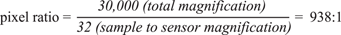 $${\rm pixel}\,{\rm ratio {\equals} }{{{\rm 30},{\rm 000 (total}\,{\rm magnification})} \over {{\rm 32 (sample }\,{\rm to}\,{\rm sensor}\,{\rm magnification})}} {\equals} {\rm 938\,\colon\,1}$$
The pixel size of the camera’s 5 MP sensor is 2.35 µm. Using the pixel ratio value of 938:1 and a 1-to-1 camera-to-monitor pixel correspondence, the monitor pixel size must be:
 $${\rm monitor}\,{\rm pixel}\,{\rm size}{\equals}938{\rm }\cdot{\rm }0.00235{\rm mm }{\equals}{\rm }2.2{\rm mm}$$
Therefore, to achieve a total magnification of 30,000:1 with a 5 MP image sensor containing 2,592 horizontal pixels, the monitor horizontal size (assuming 1,920 pixels (HD) of 2.2 mm) would be 4.2 meters (13.8 feet)! This width is more than 2.2 times larger than that of the largest monitor (1.882 m, UHD/4k) in Table 2.
But that is not the whole story. The distance the viewer is from a large monitor is also important for assessing what the viewer will see. If the viewer is too close, it is likely that the large pixels will be annoyingly visible. On the other hand, if the viewer is too far away, the finer details may be too small to see.
Range of Useful Magnification for Digital Microscopy
Now one must ask the question if this level of magnification, 30,000:1, is simply beyond the useful range, meaning it is empty magnification. How do we determine a range of useful magnification for digital microscopy when an image is observed on a monitor? First, it is important to understand the resolution or resolving power of the microscope system and the viewing distance from the monitor.
Microscope system resolution
The system resolution for a digital microscope (or stereo microscope with a digital camera) is influenced by three main factors:
(1) Diffraction-limited light microscope resolution, using Rayleigh’s criterion and the numerical aperture [9]:
 $$light\,resolution\, limit {\equals} {{ NA \cdot 10^{6} } \over {0.61 \cdot \lambda }} ({\rm line}\,{\rm pairs\,/\,mm}) $$
where NA is the numerical aperture and λ is the wavelength of light in nm.
(2) Image sensor (camera sensor) resolution [9]:
 $$sensor \,resolution\,limit{\rm {\equals}} {{500 \cdot M_{{TOT PROJ}} } \over {sensor\, bin\,mode \cdot sensor\, pixel\, size}} ({\rm line}\,{\rm pairs\,/\,mm)} $$
where M TOT PROJ is the magnification from the sample to the sensor (Equation 3), the “sensor bin mode” refers to the binning mode which is 1 for full frame (1 × 1) and 2 for 2 × 2 pixel binning, (see Figure 2a), and “pixel size” refers to the sensor pixel size in μm.
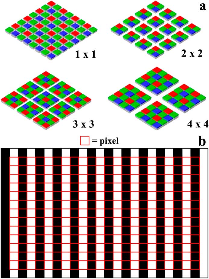
Figure 2 (a) Examples of pixel binning modes for image sensors: no binning (full frame, 1 × 1), double binning (2 × 2), triple binning (3 × 3), and quadruple binning (4 × 4). (b) Image sensor detection of black/white line pairs, used to measure the resolution limit of a microscope, requires a minimum of two pixels (red squares) per line pair (Nyquist rate). However, better image results are obtained if three or more pixels per line pair are used.
(3) Display (monitor) resolution [9]:
 $$monitor\, resolution\,limit{\rm {\equals} }{{M_{{DIS}} } \over {2 \cdot monitor\,pixel\, size}} {\rm (line}\,{\rm pairs\,/\,mm)} $$
where M DIS is the total lateral magnification (Equation 4) and the monitor pixel size is in mm.
The basis for the camera sensor and display monitor resolution limit is the Nyquist sampling theorem for digital signal processing (see Figure 2b) [14, Reference Shannon15]. This theorem assumes that at least two pixels are needed to resolve one line pair. One can simply imagine a microscope image of a sample showing line pairs projected onto the camera sensor and then displayed on the monitor. If a single line in the image corresponds to a single line of pixels, as shown in Figure 2b , say for the monitor, then to determine the minimum line pair spacing on the sample resolvable by the monitor, one can just divide the size of 2 pixels by the total lateral display magnification (M DIS ). If the same exercise is done now for the camera sensor, that is, a single line in the image corresponds to a single line of pixels, then dividing by the total projection magnification from sample to sensor (M TOT PROJ ) determines the minimum line pair spacing resolvable by the camera. To write these calculations out for more clarity:
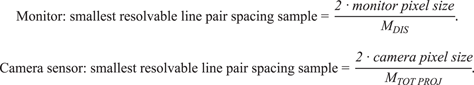 $$\eqalignno{ & {\rm Monitor\,\colon\, smallest}\,{\rm resolvable}\,{\rm line}\,{\rm pair}\,{\rm spacing}\,{\rm sample {\equals} }{{{\rm 2 \cdot monitor}\,{\rm pixel}\,{\rm size}} \over {M_{{DIS}} }}. \cr & {\rm Camera}\,{\rm sensor\,\colon\, smallest}\,{\rm resolvable}\,{\rm line}\,{\rm pair}\,{\rm spacing}\,{\rm sample {\equals} }{{{\rm 2 \cdot camera}\,{\rm pixel}\,{\rm size}} \over {M_{{TOT PROJ}} }}. \cr} $$
The reciprocal of the minimum resolvable line pair spacing gives the resolution limits shown above in Equations 7 and 8. Simply add a conversion (µm to mm) and pixel binning factor for the camera sensor to arrive at the final form of Equation 7.
For this article, as stated above, the scenario of a 1-to-1 correspondence is assumed between the pixels of the sensor and monitor. For this specific case, using Equation 4b and converting the monitor pixel size units from mm to μm, it becomes clear that the resolution limit of the sensor and monitor are identical. Example calculations demonstrating this will be given in a later section of this article.
The resolution limit of the digital microscope system resolution is determined by the smallest of the three resolution values above. The diffraction limit of the light microscope (Equation 6) still governs the ultimate level of detail that can be observed and recorded. This last point is important: the best resolution of a microscope generally is measured from a recorded image rather than a viewed image; methods for this fall outside the topics of this article [Reference Nyquist16].
Useful viewing distance
The viewing distance is the distance between the observer’s eyes and the displayed image. The range for a useful viewing distance is affected by the system resolution of the microscope and the visual angle of the observer [Reference Bradbury17, Reference Healey and Sawant18]. The minimal angle of resolution depends on the intensity of light emitted or reflected from the observed object and the contrast between its specific features. The angle ranges, on average, from 2.3 to 4.6 minutes of arc (low to high light intensity and contrast) for human eyes [9, Reference Sugawara19–Reference Hendley21]. This angular range indicates the optimal performance, in terms of visual acuity (resolution) and contrast sensitivity, of the human eye averaged over a large population varying in age from young to old. Thus, on average, an eye is capable of distinguishing details on a monitor which have a separation distance corresponding to an angular difference of 2.3 to 4.6 minutes of arc (0.038 to 0.077 degrees; 0.669 to 1.338 × 10⁻³ radians) for a specific viewing distance. To understand how the range for a useful viewing distance is determined, imagine a person observing an image displayed on a monitor which shows the smallest line pair spacing resolvable by the digital microscope system. It follows that the actual line pair spacing on the sample would then be:
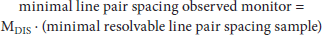 $${\rm minimal}\,{\rm line}\,{\rm pair}\,{\rm spacing}\,{\rm observed}\,{\rm monitor}{\equals}M_{{DIS}} \cdot {\rm }\left( {{\rm minimal}\,{\rm resolvable}\,{\rm line}\,{\rm pair}\,{\rm spacing}\,{\rm sample}} \right)$$
where M DIS is the total magnification (Equation 4). To determine the minimal angle of resolution for the observer’s eye necessary in order to see two separate lines in the pair, the minimal line spacing observed on the monitor must be divided by the viewing distance:
 $${\rm min}\,{\rm angle}\,{\rm resolution}\,{\rm for}\,{\rm observer} {\equals} {{M_{{DIS}} \cdot {\rm (min}\,{\rm resolvable}\,{\rm line}\,{\rm pair}\,{\rm spacing}\,{\rm sample)}} \over {viewing\,distance}} \,{\rm (radians)}.$$
The minimal resolvable line pair spacing on the sample is the inverse of the microscope system resolving power or resolution, thus:
 $$min\, angle\, resolution\, observer {\equals} {{M_{{DIS}} } \over {system \,resolution \cdot viewing\, distance}} \,{\rm (radians)}{\rm .}$$
As noted above, the minimum angle of resolution for the eye falls between 6.669 × 10⁻⁴ and 1.338 × 10⁻³ radians, so rearranging the equation above for viewing distance (in mm) and setting it equal to the lower and upper values of the angle of resolution, the useful viewing distance range can be expressed as (converted from units of mm to meters):
 $${\rm 0}{\rm .75 \cdot} {{M_{{DIS}} } \over {system \,resolution}}{\rm \,\lt\,}useful\,viewing\,distance{\rm \,\lt\, 1}{\rm .5 \cdot} {{M_{{DIS}} } \over {system \,resolution}} \,{\rm (meters)} $$
Again, M DIS is the total lateral magnification (Equation 4), and the system resolution refers to the light microscope system resolution limit as discussed above (Equations 6–8). For the following calculations, it is assumed that the viewing distance is always within the useful range.
Range of useful magnification
To understand how to determine the range of useful magnification for digital microscopy—the lowest and highest magnification values for an image displayed on a monitor where the system resolution limit is clearly observed for optimal and non-optimal illumination—it is first necessary to mention briefly the “perceived” magnification from visual observation of an image or object. Everyday experience shows that the perceived size of an object depends on the distance from which it is observed. Using geometrical optics and the relationship between angular and lateral magnification, the following can be derived:
 $$visual\, magnification{\rm {\equals} }{{M_{{DIS}} \cdot (250\, mm)} \over {viewing\, distance}} \,{\rm (no units)}$$
where M DIS is the total magnification (Equation 1) and 250 refers to the standard reference for the viewing distance in mm, which is based on the average near point for the human eye, that is, the closest point on which the eye can focus [Reference Strasburger22]. The Appendix at the end of this article provides a more detailed derivation of Equation 10.
Finally, the range of useful magnification can be defined by combining Equations 9 and 10. From Equation 10, after converting the near point of the eye from units of mm to meters:
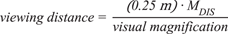 $$viewing\, distance {\rm {\equals}} {{(0.25 \,m) \cdot M_{{DIS}} } \over {visual \,magnification}}$$
Then, substituting the expression just above for the viewing distance into Equation 9 and dividing all sides by 0.25 and M DIS :
 $${{{\rm 0}{\rm .75}} \over {{\rm 0}{\rm .25 } \cdot system \,resolution}}{\rm \,\lt\, }{1 \over {useful\, magnification}}{\rm \,\lt\, }{{1.5} \over {0.25 \cdot system \,resolution}}.{\rm }$$
Now, by taking the reciprocal of the inequality, remembering to interchange the greater than and lesser than signs, the range of useful magnification is determined:
 $${{system\, resolution} \over 6}{\rm \,\lt\,} useful\, magnification{\rm \,\lt\,} {{system\, resolution} \over 3} \,{\rm (no}\,{\rm units)}$$
Thus, the range of useful magnification is between 1/6 and 1/3 of the microscope system resolution.
What does it mean exactly, the range of useful magnification? It means the optimal magnification range when observing an object via a microscope (or an optical instrument that can magnify) where the finest resolvable features can be seen. Remember that range is based on the average performance of the human eye with respect to visual acuity (resolution) and contrast sensitivity along with the optical system’s resolution limit, as mentioned above. A significant number of individuals will have eyes who perform above or below this average.
Low magnification . When the magnification from sample to camera sensor is low, generally 1× or even less, then the camera sensor or monitor are the limiting resolution factors of the microscope system. As an example, a digital microscope using a 1.6× objective (M O = 1.6×) with a numerical aperture of 0.05 (NA = 0.05), a total tube factor of 1× (q = 1×), a 0.32× photographic projection lens (M PHOT = 0.32×), a camera sensor with a 3 µm pixel size and binning mode of 1 × 1, a monitor pixel size of 0.3 mm (pixel ratio of 100:1), a 1-to-1 pixel correspondence between the sensor and monitor, and white light (mixture of all visible light wavelengths [400–700 nm] with an average in the green at λ = 550 nm) illumination, then from Equations 6, 7, and 8:
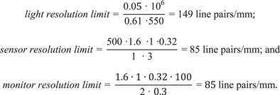 $$\eqalignno{ & light \,resolution \,limit {\rm {\equals} }{{{\rm 0}{\rm .0}5{\rm \cdot 10}^{6} } \over {{\rm 0}{\rm .61 \cdot550}}}{\rm {\equals} 149 }\,{\rm line }\,{\rm pairs\,/\,mm}\,\semi-colon\, \cr & sensor \,resolution\,limit{\rm {\equals} }{{{\rm 500 \cdot1}{\rm .6} \cdot {\rm 1 } \cdot {\rm 0}{\rm .32}} \over {1 {\rm \cdot 3}}}{\rm {\equals} 85 line }\,{\rm pairs\,/\,mm\,\semi-colon\, }\,{\rm and} \cr & monitor\, resolution\,limit{\rm {\equals} }{{1.6 \cdot 1 \cdot 0.32 \cdot 100} \over {{\rm 2 \cdot 0}{\rm .3}}}{\rm {\equals} 85 line }\,{\rm pairs\,/\,mm}. \cr} $$
This example shows that, at such low magnification, the resolution limit of camera sensors with pixels sizes larger than 2 μm (and monitors with pixel sizes larger than 0.2 mm) will start to be inferior to the light resolution. Therefore, at low magnification, approximately 1× or less, the sensor or monitor will likely be the limiting factor for the microscope system resolution.
High magnification . When the magnification from sample to camera sensor is high, generally 50× or greater, then light diffraction is the limiting resolution factor of the microscope system. Again, to illustrate it with an example, a digital microscope using a 160× objective (M O = 160×) with a numerical aperture of 1.4 (NA = 1.4), a total tube factor of one (q = 1×), a 1× photographic projection lens (M PHOT = 1×), a camera sensor with a 6 µm pixel size and binning mode of 1 × 1, a monitor pixel size of 0.3 mm (pixel ratio of 50:1), a 1-to-1 pixel correspondence between the sensor and monitor, and green light (λ = 550 nm) illumination, then from Equations 6, 7, and 8:
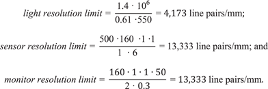 $$\eqalignno{ & light\, resolution \,limit{\rm {\equals} }{{{\rm 1}{\rm .4 \cdot 10}^{6} } \over {{\rm 0}{\rm .61 \cdot550}}}{\rm {\equals} 4,173 line }\,{\rm pairs\,/\,mm}\,\semi-colon\, \cr & sensor\, resolution \,limit{\rm {\equals} }{{{\rm 500 \cdot160} \cdot {\rm 1 } \cdot {\rm 1}} \over {1 {\rm \cdot 6}}}{\rm {\equals} 13,333 }\,{\rm line }\,{\rm pairs\,/\,mm\,\semi-colon\, }\,{\rm and} \cr & monitor\, resolution\,limit{\rm {\equals} }{{160 \cdot 1 \cdot 1 \cdot 50} \over {{\rm 2 \cdot 0}{\rm .3}}}{\rm {\equals} 13,333}\,{\rm line }\,{\rm pairs\,/\,mm}. \cr} $$
Here at high sample-to-sensor magnification, the system resolution of a microscope using a modern camera sensor with a pixel size in the 1–6 μm range (and a monitor pixels size below 0.6 mm) is limited by the light resolution.
For a best-case scenario, the greatest light resolution possible with the smallest wavelength of visible light, 400 nm, and a very high numerical aperture, 1.4, is approximately 5,740 line pairs/mm. From the example above, it is clearly seen that the resolution limit of a camera sensor with a pixel size below 6 μm easily exceeds this value.
For this description of digital microscopy, it is assumed that the image on the monitor is always observed within the range of useful viewing distance. As discussed above, the range of useful magnification is derived based on the average performance of the eye. Whenever a sample is observed with a light microscope, sample features that correspond to the microscope’s resolution limit become resolvable by the eye under optimal illumination conditions at the lower magnification value of the useful range (Equation 11). For non-optimal illumination, then the higher magnification value may be necessary for the eye to resolve the features. Beyond the higher magnification value of the range, no finer details of the sample can be resolved, so it is empty magnification.
The example above for high magnification demonstrated that the best possible resolution attained with a light microscope (objective with a 1.4 numerical aperture and illumination with 400 nm light) is about 5,740 line pairs/mm. Now, the range of useful magnification for the best resolution case can be calculated using Equation 11:
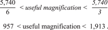 $$\eqalignno{ & {{{\rm 5,740}} \over 6}{\times}{\rm \,\lt\, }useful\, magnification{\rm \,\lt\,} {{{\rm 5,740}} \over 3}{\rm }{\times} \cr & {\rm 957 }{\times}{\rm \,\lt\, useful}\,{\rm magnification \,\lt\,} {\rm 1,913}{\times}. \cr} $$
So the highest useful magnification for a light microscope is about 1,900×–2,000×. Magnification values exceeding 2,000× fall under empty magnification. When below the lower end of the range, 957×, again it means that the average eye can no longer distinguish details on a sample with a spatial frequency equivalent to 5,740 line pairs/mm. However, most samples are not uniform with features of the same exact dimensions and spatial frequency everywhere on the surface. Normally, as magnification is decreased, other larger features with lower spatial frequencies (below the resolution limit) become resolvable.
The example for low magnification above, where the image sensor limits the resolution of the microscope (objective with a 0.05 numerical aperture and sensor with 3 µm pixel size), shows a limit of about 85 line pairs/mm. Now, the range of useful magnification for this low magnification case also can be calculated:
 $$\eqalignno{ & {{{\rm 85}} \over 6}{\times}{\rm \,\lt\,} useful\, magnification{\rm \,\lt\,} {{{\rm 85}} \over 3} {\times} \cr & {\rm 14 }{\times}{\rm \,\lt\,} useful \,magnification {\rm \,\lt\,} {\rm 28}{\times}. \cr} $$
So the range of useful magnification for this case, where the sensor limits the resolution of the microscope, is about 14× – 28×. In order to resolve features on a sample with a spatial frequency equivalent to 85 line pairs/mm, the total magnification (M DIS ) of the observed image should fall between 14× and 28×. Beyond 28× it would be empty magnification. To make sure that sample features with a spatial frequency corresponding to the resolution limit of 85 line pairs/mm can be resolved, then the choice of a monitor with appropriate dimensions and pixel size becomes important.
Object Field (Field of View)
An object field (OF) is the part of the object that is reproduced in the final image. It is also known as the microscope field of view (FOV). Thus, details of an object can only be observed if they are present within the OF. When looking through the eyepieces, the visible OF is a circular image of a portion of the sample. The size of the OF (Equation 12) is dependent on the field number (FN) of the eyepiece, as well as the magnification of the objective and tube lenses (Figure 3). In digital microscopy, the OF is rectangular because of the shape of the image sensor that collects the image and the monitor that displays it (see Figure 3). It is expressed in width and height given in mm. For digital microscopy, care has to be taken that the image created by the optical system is large enough to cover the whole image sensor. The OF can be limited either by the image sensor or the display. In either case, the physical size of the active area, given by the number of active pixels in width and height and their physical size (pixel pitch), has to be taken into account.
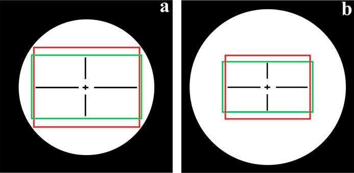
Figure 3 Diagram showing direct comparison of an image viewed through eyepieces (white circle) and simultaneously with the sensor (rectangles) of a 5 MP digital camera. The two examples shown are: (a) eyepiece with a field number (FN) of 20 mm and C-mount with 0.4× lens, and (b) eyepiece with 23 mm FN and C-mount with 0.5× lens. Some cameras detect images in a 4:3 aspect ratio (red rectangle) format for data storage and a 16:9 aspect ratio (green rectangle) format for live image output.
To calculate the OF, the physical size of the active area of the sensor (Equation 13) must be divided by either the magnification of the objective, tube, and camera projection lenses (M TOT PROJ) or, for the monitor, by the total lateral display magnification, M DIS. The smaller of these values for each width and height define the digital microscope’s OF. It is likely that both width and height of the OF are not necessarily jointly limited by the image sensor or display. For example, width can be limited by the sensor, whereas the height can be limited by the display. The final OF will depend on the dimensions and aspect ratios of the image sensor and display and the pixel correspondence (1:1, 1:2, 2:1, etc.) between them for image display. In this article, a 1-to-1 sensor pixel to monitor pixel correspondence is assumed (refer to section with Equation 5 above).
Eyepiece object field
The OF for eyepieces can be determined by:
 $$OF_{{eyepiece}} {\rm {\equals} }{{FN} \over {M_{O} \cdot q}} {\rm (mm) }$$
where OF eyepiece is the object field observed through an eyepiece, FN is the eyepiece field number in mm, and M O · q (Equation 2) is the total magnification before the eyepiece due to the objective, zoom, and any tube lenses.
Sensor object field
The OF for a camera sensor can be determined using the width and height of the sensor divided by the total magnification of the optics producing the image of the sample projected onto the sensor:
 $$w {\equals} {{pixel\,size\,\cdot \,number\, active\, pixels\, sensor\, width} \over {1000 \cdot M_{{TOT PROJ}} }} ({\rm \mu m}) $$
 $$ h {\equals} {{pixel\, size\, \cdot \,number\, active\, pixels\, sensor\, height} \over {1000 \cdot M_{{TOT PROJ}} }} ({\rm \mu m)}$$
where w and h are the width and height of the OF observed by a sensor, M TOT PROJ is the total magnification from sample to sensor (Equation 3b), and the sensor pixel size is in µm.
Figures 3 and 4 show the difference in OF between images seen by the eyepieces versus those recorded by the camera sensor, for the same sample, objective lens, and zoom setting. For Figure 4, the total magnification of the objective and zoom lens was 1×, but several types of C-mounts with different magnification were used to install the 5 MP camera on the stereo microscope. The red rectangle seen in Figure 4a represents the OF of Figure 4b, an image taken with the 0.32× C-mount. The blue rectangle indicates the OF of Figure 4c, taken with the 0.5× C-mount. The green rectangle shows the OF of Figure 4d, taken with the 0.63× C-mount. Figure 4b shows the problem of vignetting where the edges of the image are darker than the center. Vignetting almost always occurs with stereo or compound microscopes having a C-mount with too low a magnification. In that case, the image projected onto the camera sensor is smaller than the sensor size resulting in dark edges. To avoid such a problem, normally it is recommended that a 0.32× C-mount is used with a digital camera having a 4.8 × 3.6 mm sensor size, a 0.4× C-mount with a 6.1 × 4.6 mm sensor size, a 0.5× C-mount with a 8.0 × 6.4 mm sensor size, and a 0.63× C-mount with a 8.8 × 6.6 mm sensor size.
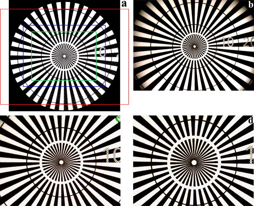
Figure 4 Images of a Siemens star taken with a stereo microscope (M205 A) having a total objective and zoom lens magnification (MO · q) of 1×. The first black line circle has a 10 mm diameter and the second a 20 mm diameter. (a) Image photographed through a 10× eyepiece with 23 mm field number (FN). Images (b–d) recorded using a digital camera installed with a C-mount (MPHOT): (b) 0.32× MPHOT and 27.2 × 20.3 mm OF; (c) 0.5× MPHOT and 17.4 × 13 mm OF; and (d) 0.63× MPHOT and 13.8 × 10.3 mm OF. The red rectangle in 4a represents the OF of 4b (0.32× C-mount), the blue the OF of 4c (0.5× C-mount), and the green the OF of 4d (0.63× C-mount).
The OF of the camera sensor can be calculated (w × h) using Equation 13a and 13b above. The range of values for the OF seen with a digital microscope and stereo microscope equipped with a digital camera are shown in Table 5.
Table 5 Object field (OF) data (Equation 13) for an image from a digital microscope with 5 MP image sensor (DMS1000) and stereo microscope (M205 A) equipped with a 5 MP digital camera (MC170 HD) showing the range from minimum to maximum values. The digital and stereo microscope discussed in this article are used often for inspection, such as during manufacturing. Generally, their maximum magnification values are lower than compound or higher performance digital microscopes.

Discussion
In planning a set of experiments, it is useful to know the lowest magnification for which the object field does not exhibit vignetting, as well as the useful range of magnification to avoid introducing empty magnification. While these issues have been described for the cases of relatively low-magnification digital microscopes and stereo microscopes, typically used for inspection during manufacturing, the same concepts can be applied to other types of light microscopes, such as compound or higher-performance digital microscopes. Indeed, the issues of magnification range and magnification values related to various monitor sizes are quite general and they are relevant to other instruments, such as scanning electron microscopes, transmission electron microscopes, and scanning probe microscopes. While the concepts would remain the same, the equations for calculating specific values of magnification would need modification.
Conclusion
Digital microscopes use electronic image sensors (camera sensors) to replace eyepieces. Microscopes for direct visual perception, such as stereo and compound microscopes, have eyepieces and can be equipped with digital cameras. Digital microscopy allows rapid acquisition of high-quality images. It is often used for fast and easy documentation, quality control (QC), failure analysis, and research and development in a variety of fields. Because of the diversity of camera sensor dimensions and electronic display monitor sizes, determining magnification and magnification range when using digital microscopy can be challenging. With this article, users of digital microscopy can better understand how to evaluate the total magnification and its useful range for a particular microscope. The useful range of magnification is dependent upon the resolution of the optical instrument and average performance of the human eye with respect to visual acuity (angular resolution) and contrast sensitivity for optimal and non-optimal illumination conditions.
Acknowledgments
We would like to thank our colleagues Reto Zìst and Harald Schnitzler of Leica Microsystems, Heerbrugg, Switzerland, for useful discussion and clarification about the many concepts and definitions concerning magnification and resolution described in the microscopy standards.
Appendix
Derivation of Equation 10:
 $$visual\, magnification {\equals} {{M_{{DIS}} \cdot (250\,mm)} \over {viewing\, distance}} ({\rm no}\,{\rm units}). $$
The diagram in Fgure A1 shows the same object being observed by a person from two different distances. One distance is the so-called “viewing distance” (d vd ) and the other is the standard reference for the viewing distance based on the average near point (d np ) of the human eye (the closest point on which the eye can focus), 250 mm [22]. The observed or perceived heights of the object are h vd at the viewing distance and h np at the eye’s near point. For rays of light coming from the top of the object and passing directly to the center of the eye’s lens in a straight line, the rays subtend an angle with respect to the horizontal of α vd for the object at the viewing distance position and α np at the eye’s near point.
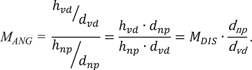
In Figure A2, an equivalent result as for Figure A1 is shown using an imaginary lens system that produces a virtual image of the object. The object is placed at the eye’s near point (d np ), and the virtual image of the object appears at the viewing distance position (d vd ). Now Figure A2 of the diagram can be analyzed using basic geometrical optics in terms of magnification. The angular magnification, M ANG , and lateral magnification, M DIS (Equation 1), for Figure A2 are:
 $$M_{{ANG}} {\rm {\equals}} {{\alpha _{{vd}} } \over {\alpha _{{np}} }} \quad {\rm and} \quad M_{{DIS}} {\equals} {{h_{{vd}} } \over {h_{{np}} }}.$$
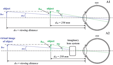
Figure A (1) Diagram showing the same object observed by the unaided eye from two different distances, the “viewing distance” and average near point of the eye (250 mm). The viewing distance is represented by d vd and the eye’s near point by d np . The perceived heights of the object are h vd at the viewing distance and h np at the eye’s near point. Light rays coming from the top of the object in the two positions subtend an angle with respect to the horizontal of α vd (viewing distance position) and α np (eye’s near point). (2) Equivalent result as A1 using an imaginary lens system that produces a virtual image of the object. The object is placed at d np , and the virtual image appears at d vd .
Considering only the case of paraxial rays, then the angle α ≈ tanα. It can also be seen from Figure A2 that:
 $$\tan (\alpha _{{vd}} ) {\equals} {{h_{{vd}} } \over {d_{{vd}} }}\,\cong\, \alpha _{{vd}} \quad {\rm and}\quad \tan (\alpha _{{np}} ) {\equals} {{h_{{np}} } \over {d_{{np}} }}\,\cong\, \alpha _{{np}} .$$
Therefore,
 $$M_{{ANG}} {\equals} {{{\raise0.7ex\hbox{${h_{{vd}} }$} \!\mathord{\left/ {\vphantom {{h_{{vd}} } {d_{{vd}} }}}\right.\kern-\nulldelimiterspace}\!\lower0.7ex\hbox{${d_{{vd}} }$}}} \over {{\raise0.7ex\hbox{${h_{{np}} }$} \!\mathord{\left/ {\vphantom {{h_{{np}} } {d_{{np}} }}}\right.\kern-\nulldelimiterspace}\!\lower0.7ex\hbox{${d_{{np}} }$}}}}{\equals}{{h_{{vd}} \cdot d_{{np}} } \over {h_{{np}} \cdot d_{{vd}} }}{\equals}M_{{DIS}} \cdot {{d_{{np}} } \over {d_{{vd}} }}.$$
Equating M ANG with the visual magnification and knowing that d np is 250 mm and d vd the viewing distance, then:
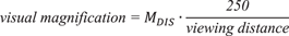 $$visual\, magnification {\equals} M_{{DIS}} \cdot {{250} \over {viewing\, distance}}$$
which is Equation 10.
For many cases, the viewing distance will be approximately the eye’s near point (d vd ≈ d np ), so:
 $$visual\,magnification\,\approx\,M_{{DIS}} .$$