Introduction
In the previous articles in this series procedures for setting up the microscope and recording SAED patterns were discussed. If the procedures are followed, the resulting SAED patterns will be well-calibrated and centered with good intensities for analysis. The patterns will also be well-suited for use in electron diffraction analysis software packages. In this last installment, software packages are discussed, and results for testing the reproducibility and reliability of SAED data acquired with these procedures are given.
Electron Diffraction Analysis Software
There are several commercial and free software packages available for the analysis of electron diffraction patterns. This author regularly uses DiffTools [Reference Mitchell1,Reference Mitchell2], CSpot [Reference Sztwiertnia and Kudłacz3], JEMS [Reference Stadelmann4], and Electron Diffraction [Reference Morniroli5] to analyze experimental spot, ring, and Kikuchi patterns. It is beyond the scope of this article to discuss all electron diffraction software packages. However, there are important features that they should include. The program should be able to simulate patterns from crystal information that is either imported or created within the software. The simulated pattern should be able to be overlaid with the diffraction pattern. The different types of diffraction patterns should be able to be indexed, for example, ring, spot, and Kikuchi patterns. It also helps to be able to interactively change the camera length to help match the pattern when the simulated pattern doesn't quite fit the experimental one. For ring patterns, it is also very useful to integrate the pattern and generate a plot that can be compared to X-ray diffraction patterns. There are three critical features that must be included in the software: pattern centering, correction of pattern distortion, and pattern calibration.
Pattern centering
To measure d-spacings and angles in diffraction patterns, the center of the pattern must be accurately positioned. The procedures outlined previously for producing a “double exposure” image provides a fiducial marker that makes pattern centering easy. DiffTools has the Locate (000) Spot command, which locates the pattern center with sub-pixel resolution by finding a geometric center of gravity for the transmitted beam. The DiffTools – Locate SADP Centre menu command can also be used to locate the pattern center. With this tool, concentric circles can be superimposed on the SAED pattern as an aid to check the results, as shown in Figure 1A. The Auto method uses a Circular Hough Transform technique to accurately find the center [Reference Mitchell6]. Figure 1B shows the manual centering of the pattern in CSpot with superimposed Au rings on the pattern. Also available in CSpot is the ability to use a circular fitting method for determining the center by positioning points on a diffraction ring (Figure 1C). The colorized zoom window helps facilitate the accurate positioning of the fitting point shown in red at the maximum intensity.

Figure 1: Centering the pattern with software. A) Centered pattern using manual adjustment in DiffTools. Three methods are available: Auto, Manual, and Center of Gravity. Concentric rings can be superimposed to help with centering the pattern. B) Manual Centering of the pattern in CSpot using the superimposed center spot Au rings. C) Pattern Centering and Corrections in CSpot. A circle or, to correct distortion, an ellipse can be fitted to the marked (111) ring to find the center of any pattern. D) Centering pattern in JEMS with superimposed rings and simulated integrated intensities. It also has a mag tool to see how well the center is set.
Correction for elliptical patterns
Not all microscopes are created equally. Distortions are possible with the lenses that might make the patterns non-circular, that is, elliptical. Of course, this will have an adverse effect on any measurements of d-spacings or angles. The tolerance on new microscopes is less than 1%, but this needs to be checked to see if distortions are present. The good news is that with digital images, the distortion can be easily measured using a polycrystalline material that generates ring patterns, as shown throughout this article. If the rings are not circular, the pattern must be corrected, and this correction can then be applied to any diffraction pattern from an unknown material [Reference Walck and Ruzakowski-Athey7]. For CSpot in Figure 1C, it is seen that there are two options to find the center from the sample points, fitting either a circle or an ellipse. Dave Mitchell has also created an Ellipse Fitting Analysis routine that can measure the elliptical distortion, save the correction parameters, and apply it to all patterns collected subsequently [Reference Mitchell and Van den Berg8,Reference Mitchell9]. This has the advantage of applying the distortion correction to any SAED pattern in DM immediately after it is recorded and prior to analyzing it with any software package.
Calibration
Obviously, the digital image must be calibrated in order to make measurements from it and to compare it to simulated phases. Anyone who has performed diffraction analyses in the TEM has been taught the derivation for the camera constant,
 $$\lambda {\rm L}{\rm} = {\rm} {\rm dD},$$
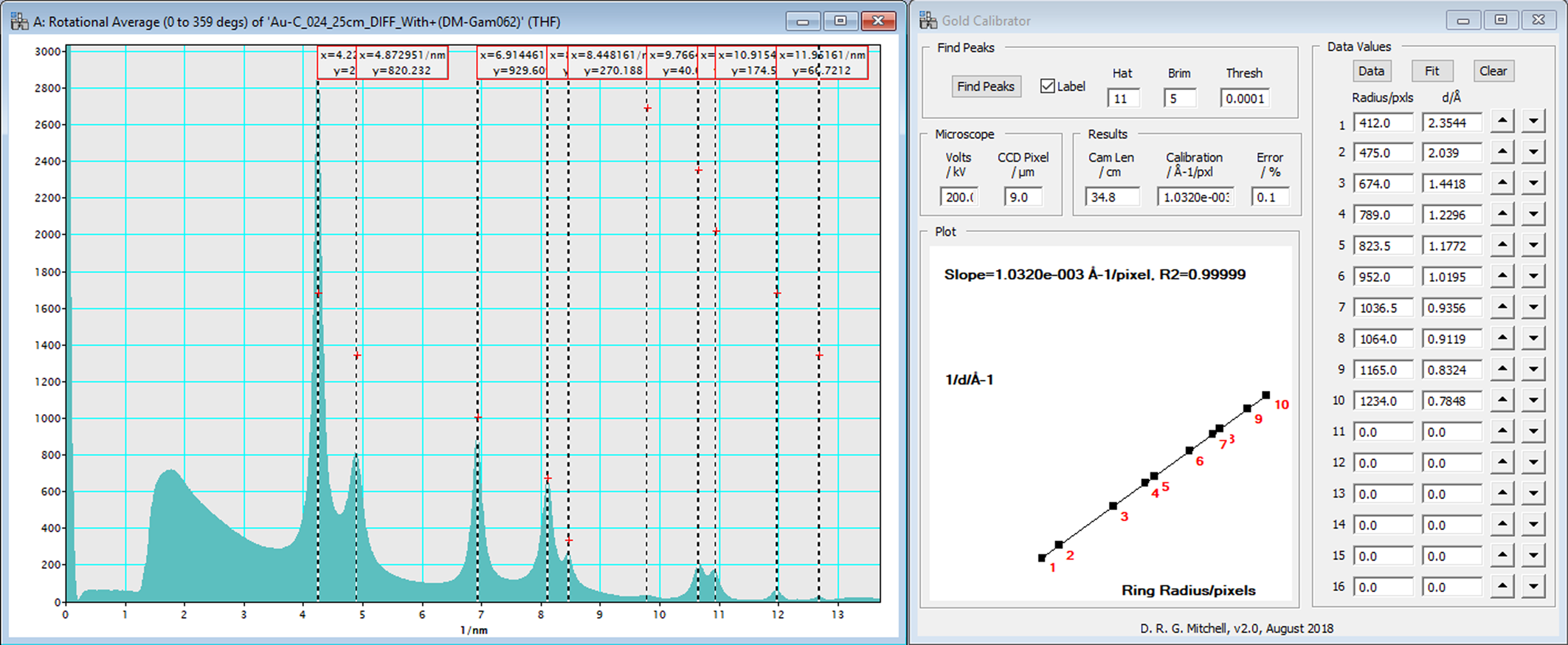
from Bragg's law, where λ is the wavelength of the electrons, L is the camera length, d is the d-spacing of a reflection, and D is the distance on the pattern from the transmitted beam to that reflection. Students are taught that we don't know either the accelerating voltage or the camera length accurately, but we do know the product of these two parameters for a known material. To determine λL, use a known material such as gold to measure the distance on the pattern from the (000) to a known reflection with a known d-spacing and multiply the two values. For digital images, λL can be measured in units of nm⋅pixels or Å⋅pixels. For example, if the size of the pixel elements of the camera is known, then λL can be converted to units of nm⋅cm. Software packages universally calculate a precise relativistic wavelength for the accelerating voltage used and then calculate the actual camera length for the nominal camera length used. An easy way that software packages calibrate the camera length is to superimpose a simulated ring pattern of the standard known material on top of an experimental ring pattern and adjust the camera length until the pattern matches, as shown in Figure 1B. DiffTools offers a gold calibration tool that works in the traditional method, where the reciprocals of the known d-spacings are plotted against the measured radius of the rings and fitted with a straight line as shown in Figure 2. From equation (1), the slope of the line is the calibration factor for the image in units of reciprocal d-spacing per pixel and is simply the reciprocal of the camera constant, λL. This approach has the benefit of giving a relative error associated with the fit, which gives an indication of the reliability for the calibration. This method will be used below to determine the reproducibility of the microscope for measuring SAED patterns using the polycrystalline gold sample. Note: for DM users, only the diameter of a single ring from a polycrystalline sample or the distance of a known reflection from a spot pattern from a single crystal pattern is used to calibrate DM (Figure 3A). Notice that DiffTools calibrates the diffraction pattern in units of Å−1, whereas units of nm−1 were chosen for DM. Differentiating thisway allows the user to know which calibration factor was used, DiffTools or DMs. If desired, the values determined by DiffTools can be used to replace the DM calibration values so that the confidence of the calibration factor is known. To do this, take the reciprocal of the calibration, divide by the relativistic wavelength, λ(Å), and multiply by the camera pixel size in mm to get the value in camera length with units of mm. This is the value that can be used in the edit box of Figure 3B for changing the calibration manually in DM. Notice the slight discrepancy in calibration values between DiffTools (1.0320 × 10⁻³ Å-1/pixel) and DM (0.010259 nm-1/pixel), which is a difference of 0.59%. DiffTools should be better because it samples the entire intensity of the rings and more than just one ring.

Figure 2: Screen capture of the Gold Calibration results from DiffTools. The slope of the line is the calibration factor measured in Å−1⋅pixels−1, which is the reciprocal of the camera constant. With the accelerating voltage and pixel resolution of the camera known, the camera length for the microscope is calculated. In this example, the nominal 25 cm camera length is actually 34.8 cm.

Figure 3: Calibration routine in DM 1.85. A) In this example, the calibration line for the (311) ring of Au is used, and half of d311 (0.12296 nm) is used to find the calibration factors. The corrected camera length and pixel size are calculated and then stored in the calibration table for the microscope. B) The Microscope-Calibrate-Image menu command to show the microscope calibration factors with the edit command insert are shown. C) Image Calibration information displayed for a SAED image in DM.
Can SAED Results Be Trusted?
Lattice parameter
After all of this, it is fair to ask several questions. How reliable is the calibration factor that is used to analyze a SAED pattern? How reliable are the measurements? How reproducible is a measurement? How often does the microscope require calibration? In preparing this article, a series of SAED patterns from a polycrystalline gold calibration standard sample were collected at two nominal camera lengths, 20 and 25 cm. Prior to each SAED pattern, the sample was moved to a random area, the “Z” position adjusted to the standard focus position, IL1 focused, the pattern centered on the crosshair, and then the long exposure and short exposure patterns acquired. Using calibration values that had been taken well over two years previously, DiffTools was used to calibrate the camera length, find the center of the pattern, perform a rotational averaged intensity profile, and find the peaks at each position. The DiffTools-Gold Calibrator routine was then used to determine the calibration factor for the pattern at the same position using the first ten peaks of the pattern. Tables 1, 2 and 3 show the resulting Au (111) d-spacings and calibration factors for the 20 and 25 cm nominal camera lengths at each of the different positions (please forgive the significant digits). For each measurement of the Au (111) d-spacing, the percent difference from the known value is shown. For the calibration factor results, the err% value is a measure of the linear fit. Using the first ten peaks in the patterns gave 0.99999 for the correlation coefficient value, R2, for every pattern measured and is therefore not shown in the tables. The tables show that the calibration factors that are over two years old still gave d-spacings that are within about 1% of the known value. In the experiment, each position required a good deal of adjustment of the “Z” position prior to acquiring apattern. Even with this, the tables show that the procedures outlined above gave very consistent results, whether measured by a d-spacing, camera length, or calibration factor. It is also interesting to note that the variation is higher for the lower camera constant. To explain this and to make it simple, let's assume that the calibration factor is known or that it has very little experimental error. To find the reciprocal d-spacing, 1/dhkl in units of Å−1 for a given (hkl) from a diffraction ring, the radius of the ring, R, in pixels is multiplied by the calibration factor for the camera length, CL, used in units of Å−1 pixels−1.
 $$\displaystyle{1 \over {d_{hkl}}} = \; C_L\; \cdot R$$
Table 1: SAED results for 20 cm camera length.
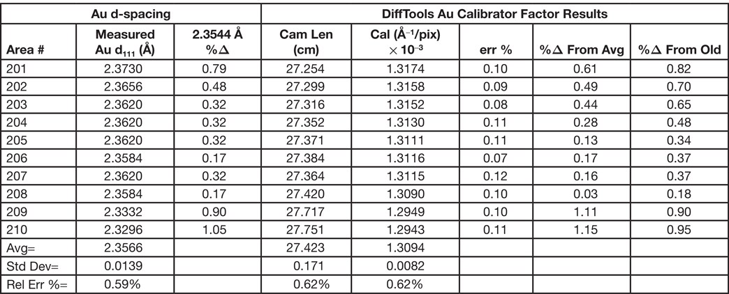
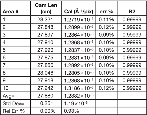
Table 2: SAED Results for 25 cm camera length.
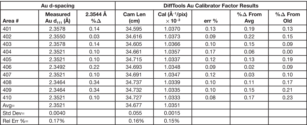
Table 3: Calibration reproducibility (20 cm) check.

The differential expression for this then becomes
 $$d\left( {\displaystyle{1 \over {d_{hkl}}}} \right) = \ln \left( {\displaystyle{1 \over {d_{hkl}}}} \right)\; d\lpar {d_{hkl}} \rpar = \; C_L\; \cdot dR$$
Considering that the lowest dR for determining the radius of the ring is one pixel, then the smallest differential for determining the d-spacing from the rotationally averaged intensity profile is given by
 $$\Delta d_{hkl} = \; \displaystyle{{C_L} \over {{\rm ln}\lpar {d_{hkl}} \rpar }}$$
For the 20 and 25 cm camera lengths, Δd111 are 0.0015 and 0.0012, respectively. Since the calibration factor, CL, will decrease as the camera length increases, the error associated with positioning of the peak will improve for a given (hkl), as the tables show. Equation 4 indicates two things should be done experimentally to improve the measurement of a sample's lattice parameters: the highest camera length and the largest reciprocal lattice vector, that is, largest possible index in the pattern, should be used. However, care must be exercised in using too high a camera length because then fewer peaks are available to determine the calibration factor in the linear fitting routine, resulting in a higher uncertainty.
Error in “Z” height positioning
Part 1 of this series of articles emphasized the importance of having the sample at the correct height with the microscope at standard focus and IL1 grabbing the back focal plane. How critical are these parameters? To investigate, a series of ten SAED patterns at different “Z” height positions were acquired, and the Au111 d-spacings and resulting calibration factors were measured. Ten random positions were first saved at the height of the original entry of the TEM holder so that the “Z” position would have to be adjusted for each pattern. The first SAED pattern was acquired at the standard position as explained above and designated the 0 nm focus. Subsequent patterns were acquired by first defocusing the objective lens by a specific amount and then changing the “Z” position until a minimum contrast condition was achieved. Then IL1 was adjusted so that the (000) spot was minimized. DiffTools was used to set the calibration of the pattern from thestored value, locate the center of the pattern, do a rotational average, and find the peaks as described above. Themeasured Au111 d-spacing was noted and then the DiffTools-Gold Calibrator routine run to find the calibration factor.
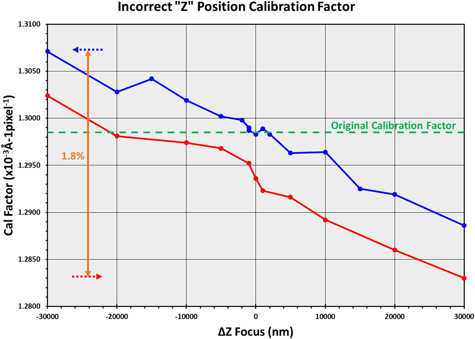
The results are shown in red in Figures 4 and 5, respectively. Two results were so surprising that the experiment was repeated a few days later, shown in blue. First, note that the difference from the true value for the Au(111) d-spacing for the worse case was only 0.22%. That is not so surprising considering the results from the tables. However, what is surprising is that the d-spacing values are within 1% from the true value, even when the “Z” position of the sample is a rather distant 30 µm away from where it should be. And, with a difference of 60 µm of positioning error, the calibration factors are within 1.8% of each other. However, what was really surprising and what caused the suspicion of something being wrong with the experiment were the four values ofd-spacings within 5 µm of the zero-focus position. All four values had the exact same values to four decimal digits, even after double-checking the calculations. Repeating the experiment gave a similar result with four values agreeing within four decimal digits, although offset from the original data, as shown in the blue curve in Figure 4. Several factors may be responsible. If Equation 4 is considered for a camera length of 20 cm, the (111) ring has too low of a ring diameter in pixels for the change in diameter to have much effect. The difference in the diameter of the ring when the sample height is changed from the zero position is probably also compensated somewhat by the refocusing of the IL1 lens. Using the (311) ring (fourth ring) gave similar results, but some differences were seen in the values when the (420) ring (eighth ring) was used.

Figure 4: Variation of Au(111) d-spacing value with the sample positioned at the incorrect height in the microscope. Red and blue curves acquired on different days.

Figure 5: Variation of calibration factor with sample positioned at the incorrect height in the microscope. Red and blue curves acquired on different days.
“Take-Aways”
There are a number of things that the reader can take away from this series of articles.
1) If the microscope is consistently set up in the same way, diffraction results can be very reliable and accurate.
2) Acquiring SAED patterns with a “double exposure” transmission beam included makes centering the pattern in diffraction analytical software much easier.
3) The lattice parameters will be a bit more accurate when a larger diameter ring (or spot) is used to calculate them. Use as large a camera length as possible, but remember that the number of rings in the standard is fewer, and so the error in the calibration factor will increase.
4) The big surprise here is how careless an operator can be and still obtain reasonable values for d-spacings. Even very large departures from the correct height position gave d-spacings that were within 1% of the true value. However, by being very careful, it was possible to obtain values that were well within 0.5%. This author usually tells users that if they get a value within 1%, be happy with it. If it is over about 1.5%, then something isn't right. Perhaps a re-evaluation of that advice is warranted.
Acknowledgements
The research reported in this document was performed in connection with contract/instrument W911QX-16-D-0014 with the U.S. Army Research Laboratory. (As of January 31, 2019, the organization is now part of the U.S. Army Combat Capabilities Development Command [formerly RDECOM] and is now called CCDC Army Research Laboratory.)
The views and conclusions contained in this document are those of the author and should not be interpreted as presenting the official policies or position, either expressed or implied, of the CCDC Army Research Laboratory or the U.S. Government unless so designated by other authorized documents. Citation of manufacturer's or trade names does not constitute an official endorsement or approval of the use thereof. The U.S. Government is authorized to reproduce and distribute reprints for Government purposes notwithstanding any copyright notation hereon.