


1 Introduction
The goal of 1% accuracy in galaxy distances is now driven more by questions in fundamental physics than astronomy. A roadmap to reach this goal exists by means of observing and modelling cosmic microwave background anisotropies (Di Valentino et al. Reference Di Valentino2018). The astronomical distance ladder also has a path to reach this goal by calibrating the Cepheid period luminosity relation and the type Ia supernova standard candle. A second population II approach exists in tip of the red giant branch (TRGB) distance measurements (Mould Reference Mould2017; Beaton et al. Reference Beaton2016).
Da Costa & Armandroff (Reference Da Costa and Armandroff1990) first showed using Milky Way globular clusters that the magnitude of the TRGB, which is set by the luminosity of the He core flash, can be used as a distance indicator for old stellar populations. Subsequent works [e.g., Hatt et al. (Reference Hatt2018), and references therein] have demonstrated the utility of the TRGB for distance determinations. Here we explore an alternative means of calibrating the TRGB method by using Gaia data release 2 (DR2) parallaxes for field red giants that lie at high Galactic latitude (Gaia Collaboration et al. Reference Brown2018b). Clementini et al. (Reference Clementini2018) present the processing and catalogues of RR Lyrae stars and Cepheids released in Gaia DR2.
2 Red Giant Sample
The ideal sample for this purpose is a stellar population drawn from the thick disk and the inner halo of the Milky Way. The density profile of the halo follows a power law with an index of order –3 out to a radius R ≈ 25–30 kpc [e.g., Saha (Reference Saha1985), Iorio et al. (Reference Iorio2018), and references therein] but has a steeper fall-off beyond this radius [e.g., Hernitschek et al. (Reference Hernitschek2018), and references therein]. This means there is little to be gained by pursuing TRGB stars to great distances, where the relative errors are larger.
2.1 Database Query
We use as our input catalogue Data Release DR1.1 of the SkyMapper survey of the southern sky (Wolf et al. Reference Wolf2018) which incorporates a crossmatch to Gaia DR2 catalogue and selected stars fainter than a SkyMapper i magnitude of 9, where saturation effects begin to appear, and brighter than Gaia G magnitude of 14 so that the Gaia image centroiding is excellent. The specific database query was:
We ran this query at ASVOFootnote a with and without the condition parallax ≥ 0.1. The colour absolute magnitude diagram (CMD) (Figure 1) was changed only at the few percent level, suggesting that statistical biases in the absolute magnitudes shown here may be modest. The rather flat distribution of parallaxes, with only a few percent negative parallaxes (Figure 2) in our CMD, is brought about by the apparent magnitude cut in G and the sparsity of stars in the outer halo. Practical guards against SkyMapper photometric saturation include the NIMA flag (the number of flagged pixels from bad, saturated, and crosstalk pixel masks) and the absence in Table 1 of stars unexpectedly red in i – z. Obviously, stars with apparently negative parallaxes have no place in Figure 1. The 3 mas cut is to control against thin disk stars, a population without a clear TRGB.

Figure 1. SkyMapper Gaia DR2 red giant branch. The axis labelled BR colour is GBP – GRP . Parallax uncertainties are shown for the brightest stars. A calibration of the TRGB by Rizzi et al. (Reference Rizzi2007) is the solid line. A Gaia DR2 mean parallax offset of –0.028 ± 0.006 mas was subtracted from the data from Table 1 of Arenou et al. (Reference Arenou2018), appropriate to the Sculptor galaxy, which is at the SGP. The dashed line represents its 6 μ as uncertainty. The query in Section 2.1 also brings in stars with luminosities fainter than are plotted here.
Figure 2. All parallaxes delivered by the query in mas units.
Table 1. Brightest stars.
Notes: NIMA is the no. of SkyMapper i flagged pixels, i_nimaflags, in the query.
axn is the astrometric excess noise in the Gaia DR2 database.
ϖ is the offset corrected parallax and σ is parallax uncertainty.
MI is the absolute I magnitude on the Cousins system.
No corrections for interstellar absorption have been applied to the SkyMapper mags.
Modifications to the query, changing the magnitude limit from 14 to 14.5 and the latitude limit from –36 to –32 bring in a few times more stars, but do not seriously change what we report in the next section. We also checked the phot_bp_rp_excess_factor and found it averaged 1.2 ± 0.1, close to the no-contamination envelope (Evans et al. Reference Evans2018). Deviant stars could be rejected from the sample. Individual reddenings can be included by appending ebmv_sfd to the query list. These values are from Schlegel et al. (Reference Schlegel1998).
2.2 Simulations
Measurement of luminosities from fluxes and parallaxes is nevertheless subject to the biases discussed by Eddington (Reference Eddington1913), Lutz & Kelker (Reference Lutz and Kelker1975), and Arenou et al. (Reference Arenou2018). Malmquist (Reference Malmquist1922) offered an analytic solution to the absolute magnitude bias resulting in an apparent magnitude limited sample of uniform density due to the larger volume accessible to the observer for brighter stars drawn from a distribution of standard candle stars with a finite dispersion. Lutz & Kelker addressed the effect of parallax errors in a similar way. The question arises as to the dispersion of the TRGB across different stellar populations and mixed stellar populations, such as that of the thick disk and halo. This has been discussed in the review by Beaton et al. (Reference Beaton2018) of distance indicators for old stellar populations. According to Serenelli et al. (Reference Serenelli2018) in the interval 10–4 < Z < 4 × 10⁻³, M bol varies by just 0.02 mag over an age range from 8.5 to 13.5 Gyr. Sweigart & Gross (Reference Sweigart and Gross1978) in the (0.7, 0.9) Mʘ total mass range M bol varies by ∼0.15 mag for a 0.1 change in the helium abundance, Y. Such a large helium spread in the halo cannot be ruled out (e.g., Milone et al. Reference Milone2018). It would be appropriate to include intrinsic dispersion in the TRGB of this order in Malmquist bias simulations and also to include the asymptotic giant branch which tends to erode the TRGB step function in the luminosity function (LF) of real stellar populations. Variations in metallicity, on the other hand, are mapped into colour variations. Fitting the TRGB to the CMD rather than the LF avoids systematic errors and Malmquist bias due to the metallicity variable. If half of all field stars are binaries, this too might be considered in estimating intrinsic dispersion. Unless the components are identical in initial mass, however, the lower mass star will still be on the main sequence and effectively invisible, when the higher mass component reaches the helium flash.
One-dimensional simulations with a power law LF terminating in the TRGB, a power law distribution of stellar distances startingFootnote b at 300 pc, a limiting flux, and a gaussian distribution of σ/ϖ whose mean absolute value is similar to that of the sample show that a quarter of the stars within 0.75 mag of the TRGB can be scattered into a region up to 0.75 mag brighter than the TRGB. Detailed 3D simulations with Galactic structure priors and an asymptotic giant branch are required to accurately correct biases of this kind. We explore this in the Appendix, using the Besancon model of stellar population synthesis (Robin et al. Reference Robin2003). Like Malmquist bias, we expect corrections to M TRGB to scale as σ 2. The reduction in σ in future Gaia data releases will markedly reduce the bias correction.
3 Analysis
3.1 The brightest stars
For stars with absolute magnitude <0, Figure 3 shows the distribution of our sample in celestial coordinates, centred on the South Galactic Pole (SGP). Gaia DR2 mean parallax offsets are discussed by Arenou et al. (Reference Arenou2018) and Chen et al. (Reference Chen2018). Adopting a single mean parallax offset for the entire sample of –0.028 ± 0.006 mas [from Table 1 of Arenou et al. (Reference Arenou2018), we collected stars with MI < –3.8 mag in Table 1.
Figure 3. Distribution of stars in Figure 1. The Small Magellanic Cloud and the cluster 47 Tuc can be seen at δ ∼ –72°.
No reddening corrections have been made to our sample, as high-latitude extinction is low (Burstein & Heiles Reference Burstein and Heiles1982; Schlegel et al. Reference Schlegel1998). The average extinction of stars in Table 1 is AI = 0.06 ± 0.002 mag.
3.2 Calibration
In population II stars with a fixed helium abundance the TRGB luminosity is predicted to be a slow rising function of metallicity (Brown et al. Reference Brown2005). The bolometric correction is a function of effective temperature, but such temperatures are difficult to establish given the extensive convective envelopes of red giant stars. So the calibration of the TRGB has tended to be an empirical matter employing filters, such as I, i and z, whose bandpasses include the peak of the Planck curve for red giants thereby reducing colour and metallicity dependence.
Bellazzini (Reference Bellazzini2007) finds
 \begin{equation} M_I^{\rm{TRGB}} = 0.08(V - I)_0^2 - 0.194(V - I{)_0} - 3.939 \end{equation}
on the Cousins photometric system. Rizzi et al. (Reference Rizzi2007) give
 \begin{equation} M_I^{\rm{TRGB}} = 0.215[(V - I{)_0} - 1.6] - 4.05, \end{equation}
which, following Hislop et al. (Reference Da Costa and Armandroff2011), we adopt. It is, however, necessary to convert the AB-mag-based SkyMapper i magnitudes to the Vega-mag-based Cousins I magnitudes. We have investigated this using photometry for the Galactic globular clusters NGC 4590 (M68) and NGC 104 (47 Tuc). Cousins V and I magnitudes for RGB stars were selected from the photometric standard star fields database maintained by StetsonFootnote c and cross-matched with both SkyMapper and Gaia DR2. Reddening correction assumed the E(B–V) values for each cluster as tabulated in the current online version of the Harris (Reference Harris1996) catalogue. In this process we assumed E(GBP – GRP ) = E(V–I) based on the effective wavelength of the filter responses.Footnote d Figure 4 then shows that for stars with GBP – GRP < 2, i.e., those where the difference in filter bandpasses does not show influence from the onset of TiO bands, is 0.435 ± 0.02 mag. We have applied this offset to the SkyMapper i mags to convert them to I mags on the Cousins system. For the same set of stars we have also investigated the relation between (V – I)0 (Cousins system) and the dereddened (GBP – GRP ) colours derived from Gaia DR2. As shown in Figure 5 a linear relation (GBP – GRP )0 = (V – I)0 + 0.15 is an adequate representationFootnote e of the relation. Figures 4 and 5 show the close relationship between Gaia colour and Cousins V – I.
Figure 4. For 99 stars with (GBP – GRP ) < 2 mag, the difference between Cousins I magnitude and SkyMapper i is 0.45 ± 0.02 mag, close to what is expected from the Vega versus AB zeropoints. In this and the following figure the axis labelled BP–RP is GBP – GRP .

Figure 5. On the Cousins V–I system (GBP – GRP )0 = (V – I)0 + 0.15 is the dashed line.
3.3 Working in parallax space
A proven solution to the biases in the astronomical distance scale that result from working in luminosity space is to invert the distance indicator or scaling relation. For example, assumed distances can be used to predict periods in the Cepheid period luminosity relation. These can then be compared with observed periods. This approach is recommended for Gaia data by Arenou et al. In the case of the TRGB there is no relation to invert, but it is still possible to work in parallax space. We calculate
 \begin{equation} \begin{array}{l} \quad \quad {\chi ^2} = \sum \frac{{{w_i}{{[{\varpi _i} - \varpi (predicted)]}^2}}}{{[\sigma _i^2 + {{({\delta _i}{\varpi _i}/2.16)}^2}]}}{(\Sigma {w_i})^{ - 1}} \\ with \ {w_i} = 1 \ {\rm{for}}|{M_i} - {\rm{TRGB}}| \lt \epsilon \\ \ and \ {w_i} = 0 \ {\rm{for}}|{M_i} - {\rm{TRGB}}| \gt \epsilon , \\ \end{array} \end{equation}
(1)
\begin{equation} \begin{array}{l} \quad \quad {\chi ^2} = \sum \frac{{{w_i}{{[{\varpi _i} - \varpi (predicted)]}^2}}}{{[\sigma _i^2 + {{({\delta _i}{\varpi _i}/2.16)}^2}]}}{(\Sigma {w_i})^{ - 1}} \\ with \ {w_i} = 1 \ {\rm{for}}|{M_i} - {\rm{TRGB}}| \lt \epsilon \\ \ and \ {w_i} = 0 \ {\rm{for}}|{M_i} - {\rm{TRGB}}| \gt \epsilon , \\ \end{array} \end{equation}
(1)
where ϖi is the star’s observed parallax, ϖ (predicted) is the prediction from the TRGB, σi is the star’s parallax error, and δi its photometric error in magnitudes. We chose values of ɛ between 0.25 and 0.5 mag and obtained clear minima close to unity in χ 2 per degree of freedom.
To eliminate the arbitrariness of ɛ we can adopt
 \begin{equation} {w_i} = {\rm{exp}}{^{ - {{[({M_i} - {\rm{TRGB}}){\varpi _i}/{\sigma _i}/2.16]}^2}}} \end{equation}
(2)
\begin{equation} {w_i} = {\rm{exp}}{^{ - {{[({M_i} - {\rm{TRGB}}){\varpi _i}/{\sigma _i}/2.16]}^2}}} \end{equation}
(2)
to downweight stars of absolute magnitude Mi in Figure 1 that are far from the TRGB. With this weighting equation 1 is a figure of merit (or demerit), rather than a χ 2 per se. Figure 6 is a map of this χ 2 in (TRGB, σ/ϖ) space where σ/ϖ is the threshold applied to parallax error for inclusion in the summation. Although the data are noisy with the present limited sample, there is evidently a minimum of χ 2 in the vicinity of TRGB = –4 mag that is fairly independent of the σ/ϖ cut.
Figure 6. Contours of χ 2 mapped against TRGB and σ/ϖ cut. There is a clear local minimum between –3.92 and –3.98 independent of parallax error cut.
Bootstrap resampling can be employed to obtain a confidence interval for TRGB at the fiducial colourFootnote f of V–I = 1.6. It is evident from Figure 6 that cutting the sample in two in σ/ϖ affects the result less than the uncertainty in the parallax offset does. This yields an uncertainty in MI for TRGB of 0.076 mag. We explored the effect of the weights in equation (2) by offsetting the input magnitudes with a small blind offset and found the local minimum in Figure 6 moved as expected.
4 Summary and future work
We find that a high-latitude Gaia DR2 CMD is consistent with the current calibration of the TRGB as an extragalactic distance indicator. This can be improved as follows:
• detailed simulations of parallax uncertainty luminosity bias,
• adding PanSTARRS photometry of high northern latitudes,Footnote g
• reducing the uncertainty in parallaxes and the parallax offset in future Gaia data releases, and
• extending the wavelength range through infrared photometry of stars with MI < –3.8 mag.
This work has made use of data from the ESA space mission Gaia, processed by the Gaia Data Processing and Analysis Consortium (DPAC). Funding for the DPAC has been provided by national institutions participating in the Gaia Multilateral Agreement. The national facility capability for SkyMapper has been funded through ARC LIEF grant LE130100104 from the Australian Research Council, awarded to the University of Sydney, the Australian National University, Swinburne University of Technology, the University of Queensland, the University of Western Australia, the University of Melbourne, Curtin University of Technology, Monash University, and the Australian Astronomical Observatory. SkyMapper is owned and operated by The Australian National University’s Research School of Astronomy and Astrophysics. The survey data were processed and provided by the SkyMapper Team at ANU. The SkyMapper node of the All-Sky Virtual Observatory (ASVO) is hosted at the National Computational Infrastructure (NCI). Development and support of the SkyMapper node of the ASVO has been funded in part by Astronomy Australia Limited (AAL) and the Australian Government through the Commonwealth’s Education Investment Fund (EIF) and National Collaborative Research Infrastructure Strategy (NCRIS), particularly the National eResearch Collaboration Tools and Resources (NeCTAR) and the Australian National Data Service Projects (ANDS). Parts of this project were conducted by the Australian Research Council Centre of Excellence for All-sky Astrophysics (CAASTRO), through project number CE110001020. Two of us are grateful for the hospitality of MIAPP, where the first draft of this paper was made and to the organizers of MIAPP’s workshop on the Extragalactic Distance Scale in the Gaia Era, Rolf Kudritzki, Lucas Macri and Sherry Suyu. This research was supported by the Munich Institute for Astro- and Particle Physics (MIAPP) of the DFG cluster of excellence ‘Origin and Structure of the Universe’. We thank Christian Wolf and Chris Onken for their help formulating and implementing the database query. We thank an anonymous referee for comments that improved the paper.
Appendix
Here we outline the parameters used to create the Besancon model (Robin et al. Reference Robin2003) that has been used to explore potential biases in the observed luminosity distribution. The model was generated to broadly resemble the underlying population from which the observed sample shown in Figure A1 was selected. The specific parameters adopted for the model were:
1. –180 ≤ l≤ +180 with steps of 30°;
2. 30 ≤ |b| ≤ 90 with steps of 30°;
3. distances between 0.3 and 50 kpc;
4. all absolute magnitudes (i.e., the default –7 ≤ MV ≤ 20 20);
5. all stellar populations [i.e., all ages from young disk (0–0.15 Gyr) through to old disk (7–10 Gyr)], thick disk, halo and bulge) with the default range of metallicities for each population;
6. spectral types from G0 to M5 with all luminosity classes included; and
7. stars selected to have 10 ≤ V ≤ 16.
Application of these parameters then resulted in a model containing 1.41 million stars. In Figure A1 we show the MI , (V – I)0 colour–magnitude diagram, on the Cousins system, for the 44 847 stars in the model that are brighter than MI = –0.5 mag. While the effects of the discrete sampling of the model are obvious, it is evident that the most luminous stars in the model are predominantly metal-poor halo RGB stars.
Figure A2 shows in black the MI LF for the stars in Figure A1 more luminous than MI = –1.5. We note that the discrete nature of the model generation process, which fundamentally uses V magnitudes, results in an uneven LF for the 0.1 mag bins used in generating the histogram—a broader binning yields a smoother function. Shown also in the figure are the results of convolving the model LF with a median parallax error amplitudes of 0.019 mas (green line) and 0.038 mas (red line). (The median parallax error xx is almost independent of magnitude for 9 < i < 11.) This confirms that parallax errors can scatter stars near the RGB tip by up to ~1 mag brighter.
Figure A1. MI , (V – I)0 colour–magnitude diagram for the 44 847 stars in the generated Besancon model that more luminous than MI = –0.5 mag. Note the predominance of the halo RGB at the brightest luminosities.
A control on this bias is available by making cuts in σ/ϖ. The lower part of Figure A2 shows the effect of cuts σ/ϖ < 0.2, 0.4. Lutz & Kelker (Reference Lutz and Kelker1975) found a similar effect with subdwarfs.
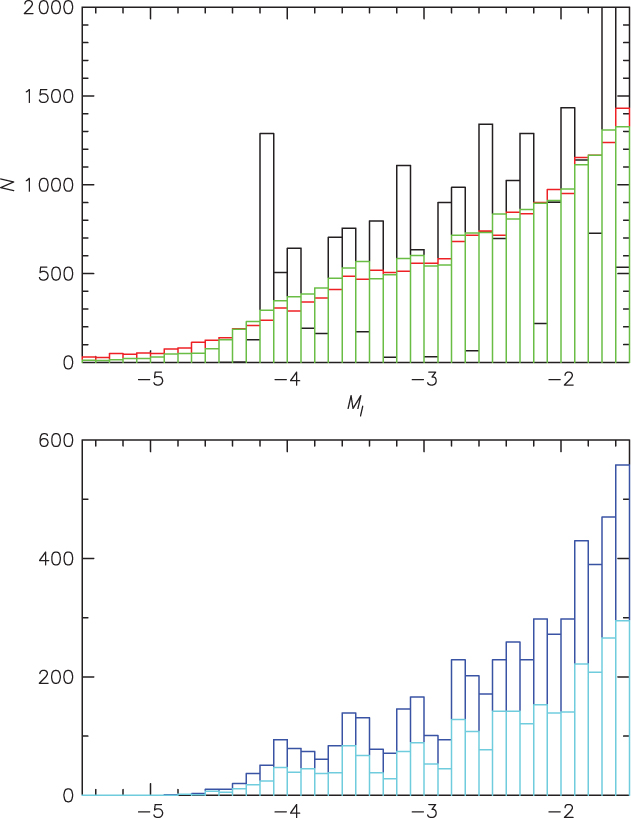
Figure A2. Black: Besancon model LF. Red: observed with a uniform distribution of parallax error amplitude ±0.02 mas. Green: ±0.01 mas. The lower panel shows the effect of cuts in σ/ϖ. Blue is σ/ϖ < 0.4. Light blue is σ/ϖ < 0.2, the ‘physics’ 5σ cut.


