2 INFERRING THE STATISTICAL PROPERTIES OF PRESTELLAR CORES FROM OBSERVATION

In well observed, nearby star-formation regions like Ophiuchus, one can identify—rather unambiguously—the small fraction of material destined to form the next generation of stars. It is concentrated in dense, low mass, self-gravitating prestellar cores, which appear to be relatively isolated from one another (Motte, Andre, & Neri Reference Motte, Andre and Neri1998; André et al. Reference André, Belloche, Motte and Peretto2007). Thus, although an individual core may continue to grow by accreting from the surrounding lower density gas, it is likely to be finished with forming stars before it interacts significantly with another neighbouring prestellar core. Therefore, it is interesting to explore the intrinsic properties of prestellar cores; to use them as the basis for detailed numerical simulations of core collapse and fragmentation (see Section 3); and to analyse how the properties of cores relate, statistically, to the properties of the stars they spawn (see Section 4).

On the basis of far-infrared and submillimetre continuum intensity maps, one can estimate the dust column-density through, and mean dust temperature along, different lines of sight through a prestellar core. Knowing the distance to the core, one then obtains the core mass, and its projected physical dimensions (i.e. projected area and aspect ratio). On the basis of molecular-line observations, one can also evaluate both the mean gas-kinetic temperature and the non-thermal component of the radial velocity dispersion. Inevitably, one does not know the distributions of density, temperature, and radial velocity dispersion along the line of sight, and one has no information on the velocity dispersion perpendicular to the line of sight. Therefore, it is impossible to construct a detailed three-dimensional model of a particular core without making a large number of extremely ad hoc assumptions.

Since the processes forming cores are chaotic, an alternative procedure is to consider a large ensemble of observed cores. With a sufficiently large number of observed cores, and assuming they are randomly oriented, one can straightforwardly deduce the distributions of mass, size, aspect ratio, temperature, and three-dimensional velocity dispersion, plus any significant correlations between these global parameters (e.g. Lomax, Whitworth, & Cartwright Reference Lomax, Whitworth and Cartwright2013). A synthetic core (or suite of cores), representing this ensemble, can then be generated by picking values from these distributions and correlations. The large-scale density profile of the synthetic core can be approximated with a critical Bonnor–Ebert profile, or a simple Plummer-like form (Whitworth & Ward-Thompson Reference Whitworth and Ward-Thompson2001)

(1) $$\begin{eqnarray} \rho (r)&=&\rho _{{\rm O}}\,\left\lbrace 1+\left(r/r_{{\rm O}}\right)^2\right\rbrace ^{-1}\,. \end{eqnarray}$$

The only remaining issue is to define the internal substructure of the synthetic core. This is critical, since it determines how the core subsequently fragments.

The procedure we have adopted is to assume that the internal non-thermal velocity field is turbulent, with power spectrum P_k ∝k ⁻ⁿ . We have adopted n = 4, but this is not very critical, as long as $3\stackrel{<}{\sim }n\stackrel{<}{\sim }5$ , since most of the power is then concentrated at short wave-numbers. In addition, we must specify the ratio of solenoidal to compressive turbulent energy, and this is critical, since it strongly influences the properties of the stars that the core spawns, as we discuss in Section 3. We also adjust the phases of the shortest wave-number solenoidal and compressive modes, i.e. those on the scale of the core, so that they are centred on the core. In other words, these modes are obliged to represent—respectively—ordered rotation and ordered radial excursions of the core; all other modes have random phases (e.g. Lomax, Whitworth, & Hubber Reference Lomax, Whitworth and Hubber2015a). Finally, we introduce fractal density perturbations, correlated with the velocity perturbations. The fractal dimension is D ≃ 2.4 and the density exponent (determining the relative amplitude of the fractal density perturbations) is dictated by the Mach Number of the turbulence.

We emphasise that there is not intended to be—indeed, there should not be—a one-to-one correspondence between the individual synthetic cores in our numerically generated ensemble, and the individual observed cores informing the distributions and correlations. They are only related in the sense that we hope they have been drawn from similar underlying distributions. Figure 1 is a grey-scale column-density image of a prestellar core generated in this way. The procedure for generating synthetic cores, and its application to the cores observed in Ophiuchus, is described in more detail in Lomax et al. (Reference Lomax, Whitworth and Cartwright2013, Reference Lomax, Whitworth, Hubber, Stamatellos and Walch2014).

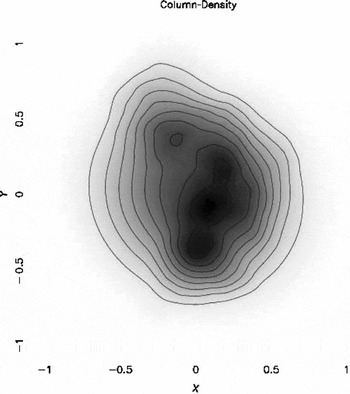
Figure 1. Grey-scale column-density image of a synthetic core.

3 SIMULATIONS OF THE COLLAPSE AND FRAGMENTATION OF PRESTELLAR CORES

We have simulated the collapse and fragmentation of an ensemble of 100 prestellar cores constructed in this way, i.e. 100 prestellar cores that, if placed at the distance of Ophiuchus and observed in dust-continuum and molecular-line radiation, would be indistinguishable statistically from the actual cores in Ophiuchus (Lomax et al. Reference Lomax, Whitworth, Hubber, Stamatellos and Walch2015b). Whether they are a good representation of the cores in Ophiuchus depends on whether the assumptions we have made in the preceding section are valid. The assumptions that turn out to be critical are (i) that the cores are randomly oriented (Lomax et al. Reference Lomax, Whitworth and Cartwright2013), (ii) the treatment of radiative feedback (Lomax et al. Reference Lomax, Whitworth, Hubber, Stamatellos and Walch2014, Reference Lomax, Whitworth, Hubber, Stamatellos and Walch2015b, see below), and (iii) the ratio of solenoidal to compressive turbulence (Lomax et al. Reference Lomax, Whitworth and Hubber2015a). Our assumptions about the density profile, the fractal dimension, and the density- and velocity-scaling exponents appear to be much less critical, in the sense that they do not greatly influence the properties of the stars that form in the simulations. We note that the observed non-thermal kinetic energies in the Ophiuchus cores—here interpreted as isotropic turbulence—are typically much smaller than their gravitational potential energies, specifically

(2) $$\begin{eqnarray} \alpha _{{\rm NON-THERM}}&=&\frac{E_{{\rm NON-THERM}}}{\left|E_{{\rm GRAV}}\right|}\;\,\stackrel{<}{\sim }\;\,0.1\,. \end{eqnarray}$$

The associated non-thermal velocities are typically trans-sonic.

The simulations use the seren ∇h-SPH code (Hubber et al. Reference Hubber, Batty, McLeod and Whitworth2011), with η = 1.2 (so a particle typically has ~ 56 neighbours). Gravitational forces are computed using a tree, and the Morris & Monaghan (Reference Morris and Monaghan1997) formulation of time-dependent artificial viscosity is invoked. In all simulations, an SPH particle has mass m _SPH = 10⁻⁵ M_⊙, so the opacity limit (~ 3 × 10⁻³ M_⊙) is resolved with ~ 300 particles. Gravitationally bound regions with density higher than ρ_SINK = 10⁻⁹ g cm⁻³ are replaced with sink particles (Hubber, Walch, & Whitworth Reference Hubber, Walch and Whitworth2013). Sink particles have radius r _SINK ≃ 0.2 AU, corresponding to the smoothing length of an SPH particle with density equal to ρ_SINK. The equation of state and the energy equation are treated with the algorithm described in Stamatellos et al. (Reference Stamatellos, Whitworth, Bisbas and Goodwin2007b), which captures approximately the effects of radiation transport.

Radiative feedback from protostars is also included, using two distinct prescriptions. In the first prescription, labelled continuous feedback, accretion onto a protostar is presumed to occur at the same rate at which matter is assimilated by the associated sink, so the stellar luminosity is

(3) $$\begin{eqnarray} L_\star &\sim &\frac{GM_{{\rm SINK}}\dot{M}_{{\rm SINK}}}{3R_{\odot }}\,. \end{eqnarray}$$

Here, M _SINK is the mass of the sink, $\dot{M}_{{\rm SINK}}$ is the rate at which the sink is growing due to accretion, and 3R _⊙ is the approximate radius of a low-mass protostar (Palla & Stahler Reference Palla and Stahler1993). In the second prescription, labelled episodic feedback, we use the phenomenological ‘sub-sink’ accretion model described in Stamatellos, Whitworth, & Hubber (Reference Stamatellos, Whitworth and Hubber2011)—and also used in Stamatellos, Whitworth, & Hubber (Reference Stamatellos, Whitworth and Hubber2012) and Lomax et al. (Reference Lomax, Whitworth, Hubber, Stamatellos and Walch2014). In this phenomenological model, which is based on the theory developed by Zhu et al. (Reference Zhu, Hartmann and Gammie2009), highly luminous, short-lived accretion bursts are separated by long intervals of low accretion and low luminosity. During the long intervals, matter collects in the inner accretion disc inside a sink, but the rate of accretion onto the central primary protostar is low—basically because there is no effective mechanism for redistributing angular momentum: the matter in the inner accretion disc is too hot for gravitational structures to develop and exert torques, and too cool to be thermally ionised and couple to the magnetic field. Consequently, the luminosity of the central primary protostar is also low, and the disc cools down and may become cool enough to fragment. Once sufficient matter has collected in the inner accretion disc, it becomes hot enough for thermal ionisation to be significant; the Magneto-rotational instability then cuts in, delivering efficient outward angular momentum transport; matter is dumped onto the protostar giving an accretion outburst and an associated peak in the luminosity, which heats the disc and stabilises it against fragmentation.

Each of the 100 cores in the ensemble has been evolved numerically with both continuous and episodic radiative feedback, and with different proportions of solenoidal and compressive turbulence (Lomax et al. Reference Lomax, Whitworth, Hubber, Stamatellos and Walch2014, Reference Lomax, Whitworth and Hubber2015a, Reference Lomax, Whitworth, Hubber, Stamatellos and Walch2015b). The simulations reproduce very well the observed mass function of young stars, and their multiplicity properties, including the incidence of high-order hierarchical multiples, but only if at least ~ 30% of the turbulent kinetic energy is in solenoidal modes, and only if the radiative feedback from protostars is episodic.

Some solenoidal turbulent energy is required, to promote the formation of massive extended circumstellar discs around the first protostars to form, and episodic feedback is required to allow these discs to periodically become sufficiently cool to fragment gravitationally and spawn additional protostars, in particular brown-dwarf protostars.

If there is no solenoidal turbulence, the circumstellar discs around the first protostars to form (which by the end of the simulation are usually the most massive protostars) are compact and unable to fragment. Low-mass protostars still form, by fragmentation of the filaments that feed material towards these more massive protostars, but very few of these low-mass protostars end up below the hydrogen-burning limit, and so in the end, there are far too few brown-dwarf protostars to match observationsFootnote ¹ . As the amount of solenoidal turbulence increases, the mean stellar mass decreases, and the fraction of brown dwarfs increases.

Even if there is solenoidal turbulence (and so extended massive circumstellar discs do form around the first protostars), as long as there is continuous feedback, the discs are warm and disc fragmentation is effectively suppressed. Consequently, the first protostars tend to accrete all the mass in their circumstellar discs and become very massive. Again, the upshot is that the mean stellar mass is high and there are very few brown dwarfs. Moreover, the few brown dwarfs that do form are very close to the hydrogen-burning limit, and there are none close to the deuterium-burning limit. Episodic accretion allows circumstellar discs to cool down, and—provided that the duty-cycle for episodic accretion is sufficiently long, i.e comparable with or greater than the dynamical timescale of the outer parts of the disc, say $\stackrel{>}{\sim }3\,000\,{\rm yrs}$ —the discs are cool enough for long enough to fragment, thereby spawning brown dwarfs and low-mass hydrogen-burning stars. Recent estimates of the duty-cycle for episodic accretion indicate that it may indeed be this long (e.g. Scholz, Froebrich, & Wood Reference Scholz, Froebrich and Wood2013).

Disc fragmentation is also conducive to the formation of hierarchical (and therefore stable) higher order multiples, and our simulations with solenoidal turbulence and episodic feedback deliver distributions of binaries and higher order multiples that are in good agreement with observation, including systems with up to six components. Figure 2 illustrates an hierarchical sextuple system formed in one of our simulations. If there is too little solenoidal turbulence, and/or more continuous radiative feedback, far too few multiple systems are formed.

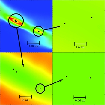
Figure 2. Montage of false-colour column-density maps of the central regions of a collapsed core which has formed an hierarchical sextuplet. The protostars are marked with black dots.

With continuous radiative feedback, an average core spawns between one and two protostars; with episodic feedback this increases to between four and five protostars. This is a controversial result, in the sense that it has usually been assumed that a core typically forms one or two protostars, with the majority of the core mass then being dispersed. However, there are good statistical reasons to suggest that a typical core may well spawn between four and five protostars (see Section 4 and Holman et al. Reference Holman, Walch, Goodwin and Whitworth2013). There are also recent observations implying that the number of protostars in a core has been underestimated. Additionally, the fact that young populations include significant numbers of high-order multiples suggests that cores must, at least occasionally, spawn many more than two protostars (e.g. Kraus et al. Reference Kraus, Ireland, Martinache and Hillenbrand2011).

A key factor promoting the formation and gravitational fragmentation of discs in simulations with solenoidal turbulence is that the infall onto a circumstellar disc is seldom smooth. The discs form in a very dynamic environment, in which new material is often delivered to a disc quite impulsively, i.e. at an abruptly increased rate, and/or along a filament whose direction and interception point bear little relation to the structure and orientation of the existing disc. Discs are also occasionally perturbed tidally by close passages of other protostars that have formed in the disc, an occurrence that is more frequent if cores spawn between four and five protostars.

As well as promoting disc fragmentation, these perturbations represent a stochastic and impulsive input of angular momentum. This has the consequence that discs can be quite poorly aligned with the spins of their central stars, as shown by Bate, Lodato, & Pringle (Reference Bate, Lodato and Pringle2010), and that the spins of stars in multiple systems are often rather poorly aligned with one another and with their mutual orbits (e.g. Lomax et al. Reference Lomax, Whitworth, Hubber, Stamatellos and Walch2015b).

4 THE STATISTICS OF CORE FRAGMENTATION

It has frequently been noted that the prestellar core mass function (hereafter CMF) is similar in shape to the stellar initial mass function (hereafter IMF)—basically log-normal with a power-law tail at high masses—but shifted to higher masses by a factor of 4 ± 1 (e.g. André et al. Reference André2010). This has led to the hypothesis that the shape of the IMF is inherited directly from the CMF. If this inference is correct, then the mapping from the CMF to the IMF must be statistically self similar. In other words, for a core of any mass M CORE, the mean fraction of the core’s mass that ends up in protostars (ηO), the mean number of protostars formed from the core ( ${\cal N}_{{\rm O}}$ ), the distribution of relative stellar masses (which we here characterise as a log-normal with standard deviation σO), and the predisposition of these protostars to end up in binaries or higher order multiples (which we here characterise with an exponent αO such that the relative probability for a protostar of mass M ⋆ to end up in a binary is proportional to M αO ⋆) are all universal.Footnote 2 For example, the probability that a core with mass 0.5 M⊙ spawns two protostars with masses between 0.1 and 0.2 M⊙ is the same as the probability that a core with mass 5 M⊙ spawns two protostars with masses between 1 and 2 M⊙.

Holman et al. (Reference Holman, Walch, Goodwin and Whitworth2013) have used a Monte Carlo Markov Chain analysis to determine which parameter values deliver an acceptable mapping between the observed distribution of core mass and the observed distributions of stellar mass, binary frequency (as a function of primary mass), and binary mass ratio (as a function of primary mass). This analysis predicts—very ‘forcefully’—that the preferred value of η_O is η_O ≃ 1.0 ± 0.3, i.e. most of the initial core mass ends up in protostars. We note that η_O > 1 is admissible, because, between the time when the mass of a core is measured and the time when it has finished forming protostars, the core can—and almost certainly does—accrete additional matter. The preferred value of ${\cal N}_{{\rm O}}$ is ${\cal N}_{{\rm O}}\simeq 4.3\pm 0.4$ (as predicted by the numerical simulations described in Section 3), so that the shift from the peak of the IMF to the peak of the CMF should be ${\cal N}_{{\rm O}}/\eta _{{\rm O}}\simeq 4.3\pm 1.3$ (as observed). The basic reason why ${\cal N}_{{\rm O}}\sim 4\;{\rm to}\;5$ fits the observations so much better than ${\cal N}_{{\rm O}}\sim 1\;{\rm to}\;2$ is that the former predicts that the binary frequency increases monotonically with primary mass, almost exactly as observed (see Figure 3), whereas the latter predicts that the binary frequency decreases with primary mass.

Figure 3. The dashed line gives the binary frequency as a function of primary mass for the best-fitting values of η_O ≃ 1.0, ${\cal N}_{{\rm O}}\simeq 4.3$ , σ_O ≃ 0.30 and α_O ≃ 0.9 identified by the Monte Carlo Markov Chain analysis. The boxes represent the observational estimates of multiplicity frequency in different primary-mass intervals, due to Close et al. (Reference Close, Siegler, Freed and Biller2003); Basri & Reiners (Reference Basri and Reiners2006); Fischer & Marcy (Reference Fischer and Marcy1992); Duquennoy & Mayor (Reference Duquennoy and Mayor1991); Preibisch et al. (Reference Preibisch, Balega, Hofmann, Weigelt and Zinnecker1999); Mason et al. (Reference Mason, Gies, Hartkopf, Bagnuolo, ten Brummelaar and McAlister1998). The error bars represent the observational uncertainties.

The preferred value of σ_O is σ_O ≃ 0.30 ± 0.03, so the interquartile range for the protostars spawned by a single core spans a factor of order 2.

Finally, the preferred value of α_O is α_O ≃ 0.9 ± 0.6, meaning that there is some dynamical biasing, i.e. some tendency for the more massive protostars to end up in binaries, but rather weaker than the results of pure N-body simulations (McDonald & Clarke Reference McDonald and Clarke1995) would suggest. This implies that the protostars in a core do not form first and then pair up. Rather, the identity of a future companion protostar is determined during formation. For example, our simulations of Ophiuchus-like cores suggest that companions to the more massive protostars often form by disc fragmentation.

These aspects of protostar formation, and those discussed in Section 3, all indicate that the notion of an isolated primary protostar with a symmetric infalling envelope and a symmetric circumstellar disc may be misleading. Circumstellar (and circumbinary) discs probably form in chaotic environments, where impulsive perturbations due to anisotropic lumpy accretion streams and nearby passing protostars are the norm.

5 THE BASIC THEORY OF DISC FRAGMENTATION

Consider an equilibrium circumstellar disc with surface-density Σ(R), isothermal sound-speed c _S(R), angular speed Ω(R) and epicyclic frequency κ(R). As long as the overall mass of the disc is less than the mass of the central protostar, we can put

(4) $$\begin{eqnarray} \kappa (R)\;\,\rightarrow \;\,\Omega (R)&\sim &\left(\frac{GM_\star }{R^3}\right)^{1/2}\,, \end{eqnarray}$$

(and henceforth the variable κ will be used exclusively for opacity). In the sequel, we shall not normally include the R-dependence of Σ(R), c _S(R), and Ω(R) explicitly.

Now, suppose that a small circular patch of the disc at radius R, having radius r ≪ R (i.e. a proto-fragment), becomes unstable and starts to condense out. The radial excursions of this proto-fragment are dictated by the balance between gravitational, pressure, and centrifugal accelerations,

(5) $$\begin{eqnarray} \ddot{r}&\;\sim \;&-\,2\pi G\Sigma \,+\,\frac{c_{{\rm S}}^2}{r}\,+\,\Omega ^2r\,. \end{eqnarray}$$

Condensation requires $\ddot{r}<0$ , and so the range of unstable proto-fragment radii, (r _MIN, r _MAX), is given by

(6) $$\begin{eqnarray} r_{{\rm MIN,MAX}}&\sim &\frac{\pi G\Sigma \,\mp \,\left\lbrace (\pi G\Sigma )^2-(c_{{\rm S}}\Omega )^2\right\rbrace ^{1/2}}{\Omega ^2}\,. \end{eqnarray}$$

There are real roots, and therefore there are only unstable proto-fragments at radius R, if πGΣ > c _SΩ, i.e.

(7) $$\begin{eqnarray} \Sigma >\Sigma _{\rm MIN}\;\sim \;\frac{c_{\rm S}\Omega }{\pi G}\,. \end{eqnarray}$$

This is the Toomre criterion for gravitational instability of an equilibrium disc (Toomre Reference Toomre1964).

We note that proto-fragments with r < r _MIN are unable to condense out because their pressure support is stronger than their self-gravity. In contrast, proto-fragments with r > r _MAX are unable to condense out because their rotational support is stronger than their self gravity.

The timescale on which a proto-fragment condenses out is

(8) $$\begin{eqnarray} \nonumber t_{{\rm COND}}&\sim &\left(\frac{2r}{\ddot{r}}\right)^{1/2}\\ &\sim &\left\lbrace \frac{\pi G\Sigma }{r}-\frac{c_{{\rm S}}^2}{2r^2}-\frac{\Omega ^2}{2}\right\rbrace ^{\!-1/2}\,, \end{eqnarray}$$

and the fastest condensing fragment has

(9) $$\begin{eqnarray} \nonumber r_{{\rm FAST}}&\sim &\frac{c_{{\rm S}}^2}{\pi G\Sigma }\,, \\ t_{{\rm FAST}}&\sim &\left\lbrace \frac{(\pi G\Sigma )^2}{2c_{{\rm S}}^2}-\frac{\Omega ^2}{2}\right\rbrace ^{\!-1/2} \end{eqnarray}$$

(10) $$\begin{eqnarray} &\sim &\frac{t_{{\rm ORB}}}{2^{1/2}\pi \left\lbrace (\Sigma /\Sigma _{{\rm MIN}})^2-1\right\rbrace ^{\!1/2}}\,, \end{eqnarray}$$

where

(11) $$\begin{eqnarray} t_{{\rm ORB}}&=&\frac{2\pi }{\Omega } \end{eqnarray}$$

is the orbital period at radius R. Thus, a proto-fragment can condense out in one orbital period if

(12) $$\begin{eqnarray} \frac{\Sigma }{\Sigma _{{\rm MIN}}}&\stackrel{>}{\sim }&1\,+\,\frac{1}{(2\pi )^2}\;\,\sim \;\,1.025; \end{eqnarray}$$

this implies that the disc need only be marginally unstable for proto-fragments to condense out on an orbital timescale.

6 HOW FAST MUST A PROTO-FRAGMENT LOSE THERMAL ENERGY TO CONDENSE OUT?

In what follows, we shall substitute for the temperature in terms of the isothermal sound-speed, c _S, viz.

(13) $$\begin{eqnarray} T&\longrightarrow &\frac{\bar{m}\,c_{{\rm S}}^2}{k_{{\rm B}}}\,, \end{eqnarray}$$

where $\bar{m}$ is the mean gas-particle mass (which for molecular gas is $\bar{m}\sim 5\times 10^{-24}\,{\rm g}$ ) and k _B is Boltzmann’s constant. The flux from a blackbody is then

(14) $$\begin{eqnarray} F_{{\rm BB}}&=&\sigma _{{\rm B}}\,T^4\;\,=\;\,\frac{2\,\pi ^5\,\bar{m}^4\,c_{{\rm S}}^8}{15\,c_{{\rm L}}^2\,h^3}\,, \end{eqnarray}$$

where σ_B is the Stefan–Boltzmann constant, and c _L is the speed of light.

A proto-fragment in a disc can only condense out if it can cool radiatively, on a dynamical timescale. Otherwise it will undergo an adiabatic bounce, and be sheared apart or merge with another proto-fragment. We shall assume that cooling is dominated by thermal emission from dust.

The frequency-averaged mass-opacity for a standard mixture of interstellar gas and dust (at the long wavelengths of concern here) can by approximated by

(15) $$\begin{eqnarray} \bar{\kappa }_{{\rm R}}&\sim &\kappa _{_T}\,T^2\;\,\sim \;\,\kappa _{{c}}\,c_{{\rm S}}^4\,, \end{eqnarray}$$

with κ _T ≃ 10⁻³ cm² g⁻¹ K⁻² and $\kappa _{_c}=\kappa _{_T}(\bar{m}/k_{{\rm B}})^2\simeq 1.2\times 10^{-18}\,{\rm s}^4\,{\rm cm}^{-2}\,{\rm g}^{-1}\,$ . The uncertainty on these coefficients is the same as on, say, the mass-opacity that is routinely used to estimate column-densities from 850 μm intensities, i.e. a factor of order two. For simplicity, we do not distinguish between the Rosseland- and Planck-mean opacities.

At the temperatures with which we are concerned here, $T\stackrel{<}{\sim }100\,{\rm K}$ , the rotational and vibrational degrees of freedom of a hydrogen molecule are not significantly excited, and therefore the gas is effectively monatomic, with specific internal energy u = 3c ² _S/2. If we assume that the dynamical timescale for a condensing proto-fragment in a disc is the same as its orbital period, then the requirement that a proto-fragment be able to cool on a dynamical timescale becomes

(16) $$\begin{eqnarray} \frac{3\Sigma c_{{\rm S}}^2/2}{t_{{\rm ORB}}}&\,<\,&\left\lbrace \begin{array}{ll}2F_{{\rm BB}}\bar{\tau }\,,\hspace{14.22636pt}&\bar{\tau }<1\;{\rm (optically\;thin)}\,,\hspace{28.45274pt}\\ 2F_{{\rm BB}}\bar{\tau }^{-1}\,,&\bar{\tau }>1\;{\rm (optically\;thick)}\,, \end{array}\right. \end{eqnarray}$$

(17) $$\begin{eqnarray} \nonumber \\ \bar{\tau }&=&\frac{\Sigma \bar{\kappa }}{2}\,, \end{eqnarray}$$

which is equivalent to the Gammie Criterion (Gammie Reference Gammie2001). The Gammie Criterion has been confirmed numerically by various groups, usually using a parameterised cooling law of the form dln [u]/dt = −2π/βt _ORB, e.g. Rice et al. (Reference Rice, Armitage, Bate and Bonnell2003), although there is still some debate as to the validity of the Gammie Criterion (see, for example, Meru & Bate Reference Meru and Bate2011; Rice et al. Reference Rice, Paardekooper, Forgan and Armitage2014). The Gammie Criterion is basically the same as the Opacity Limit (e.g. Rees Reference Rees1976; Low & Lynden-Bell Reference Low and Lynden-Bell1976), but formulated for the case of two-dimensional fragmentation of a disc (Toomre instability), rather than three-dimensional fragmentation of an extended three-dimensional medium (Jeans instability). We will return to the reason why the dynamical timescale of a proto-fragment might be the same as its orbital timescale in Section 9.

7 THE BROWN DWARF DESERT

7.1. The optically thin limit

If we adopt the first option in Equation (16), i.e. that the proto-fragment is optically thin to its own cooling radiation, and substitute from Equations (11), (14), (15), and (17), we obtain

(18) $$\begin{eqnarray} \frac{45c_{{\rm L}}^2h^3\Omega }{8\pi ^6\bar{m}^4\kappa _{{\rm c}}c_{{\rm S}}^{10}}&\stackrel{<}{\sim }&1\,. \end{eqnarray}$$

Using Equation (4) to replace Ω, this reduces to

(19) $$\begin{eqnarray} \nonumber R\,\stackrel{>}{\sim }\,R_{{\,\rm MIN}}^{^{\rm OPT.THIN}}&\!\sim \!&\left(\!\frac{3c_{{\rm L}}\bar{m}GM_\star c_{{\rm S}}}{5\kappa _{{\rm c}}^2}\!\right)^{\!1/3}\frac{15h^2c_{{\rm L}}}{4\pi ^4\bar{m}^3c_{{\rm S}}^7}\\ \nonumber &\!\sim \!&\,70\,{\rm AU}\left(\!\frac{M_\star }{{\rm M}_{\odot }}\!\right)^{\!1/3}\left(\frac{c_{{\rm S}}}{0.2\,{\rm km}\,{\rm s}^{-1}}\right)^{\!-20/3},\\ \end{eqnarray}$$

which might seem to imply that proto-fragments can condense out at any radius where the disc is optically thin, provided the gas is hot enough (sufficiently large c _S).

However, if the optically thin limit is to obtain, the surface-density must not be too large,

(20) $$\begin{eqnarray} \nonumber \Sigma \;\,\stackrel{<}{\sim }\;\,\Sigma _{\tau =1}&\sim &\frac{2}{\kappa _{{\rm c}}c_{{\rm S}}^4}\\ &\sim &10\,{\rm g}\,{\rm cm}^{-2}\left(\frac{c_{{\rm S}}}{0.2\,{\rm km}\,{\rm s}^{-1}}\right)^{-4}. \end{eqnarray}$$

Consequently, the initial radii and masses of proto-fragments must satisfy

(21) $$\begin{eqnarray} \nonumber r_{{\rm FRAG}}\;\stackrel{>}{\sim }\;r_{\tau =1}&\sim &\frac{\kappa _{{\rm c}}c_{{\rm S}}^6}{2\pi G}\\ &\sim &14\,{\rm AU}\left(\frac{c_{{\rm S}}}{0.2\,{\rm km}\,{\rm s}^{-1}}\right)^6, \end{eqnarray}$$

(22) $$\begin{eqnarray} \nonumber m_{{\rm FRAG}}\;\stackrel{>}{\sim }\;m_{\tau =1}&\sim &\frac{\kappa _{{\rm c}}c_{{\rm S}}^8}{2\pi G^2}\\ &\sim &0.001\,{\rm M}_{\odot }\left(\frac{c_{{\rm S}}}{0.2\,{\rm km}\,{\rm s}^{-1}}\right)^8.\hspace{28.45274pt} \end{eqnarray}$$

A proto-fragment with radius and mass obeying these constraints [Equations (21) and (22)]marginally, can only avoid being disrupted by the tidal field of the central protostar if it is formed at

(23) $$\begin{eqnarray} \nonumber R\;\stackrel{>}{\sim }\;R_{\tau =1}^{^{\rm TIDAL}}&\sim &\left(\frac{\kappa _{{\rm c}}^2M_\star c_{{\rm S}}^{10}}{(4\pi )^2 G}\right)^{1/3}\\ &\sim &70\,{\rm AU}\left(\!\frac{M_\star }{{\rm M}_{\odot }}\!\right)^{\!1/3}\left(\frac{c_{{\rm S}}}{0.2\,{\rm km}\,{\rm s}^{-1}}\right)^{10/3}\!;\hspace{22.76228pt} \end{eqnarray}$$

and, if it obeys them more conservatively, it has to form even further out from the central protostar.

Evidently, it is hard for optically thin proto-fragments to condense out if the gas in the disc is much hotter than 10 K (c _S ~ 0.2 km s⁻¹). For example, a modest temperature increase to 20 K (c _S ~ 0.3 km s⁻¹) increases the critical tidal radius [Equation (23)] to R ^TIDAL _{τ = 1} ~ 200 AU, and the minimum proto-fragment radius [Equation (21)] to r ^OPT.THIN _{τ = 1} ~ 110 AU. Even setting aside the assumption implicit in our analysis, that a proto-fragment be much smaller than the distance to the central primary protostar, this would require the disc to extend to ~ 300 AU, with surface-density of order 10 g cm⁻², and hence a rather large disc mass $M_{{\rm DISC}}\stackrel{>}{\sim }{\rm M}_{\odot }$ . Any further temperature increase would make fragmentation of an optically thin part of the disc very unlikely.

In other words, at radii where a disc has sufficiently low surface-density and/or sufficiently low temperature to be optically thin, proto-fragments are so extended, and hence so susceptible to tidal disruption by the central protostar, that they are unlikely to survive—unless they are far from the central protostar, i.e. at radii satisfying Equation (23). Equation (23) defines the sweet spot for fragmentation of optically thin regions in a disc. Consideration of the extents of observed discs ( $R\stackrel{<}{\sim }300\,{\rm AU}$ ) then implies that fragmentation is only likely if the temperature is low, T ~ 10 to 20 K (c _S ~ 0.2 to 0.3 km s⁻¹) at radii $R\stackrel{>}{\sim }70\,{\rm AU}$ .

7.2. The optically thick limit

Conversely, if we adopt the second option in Equation (16), i.e. that the proto-fragment is optically thick to its own cooling radiation, then substituting from Equations (11), (14), (15), and (17), we obtain

(24) $$\begin{eqnarray} \Sigma &\stackrel{<}{\sim }&\Sigma _{{\rm MAX}}^{^{\rm OPT.THICK}}\;\,\sim \;\,\left(\frac{2}{5h^3\kappa _{{\rm c}}\Omega }\right)^{1/2}\frac{4\pi ^3\bar{m}^2c_{{\rm S}}}{3c_{{\rm L}}}.\hspace{28.45274pt} \end{eqnarray}$$

In order to satisfy Equations (7) and (24) simultaneously, we require Σ_MIN < Σ ^OPT.THICK _MAX, and, since both Σ_MIN and Σ ^OPT.THICK _MAX are linear in c _S, we are left with

(25) $$\begin{eqnarray} \Omega &\stackrel{<}{\sim }&\left(\frac{32\pi ^8G^2\bar{m}^4}{45h^3c_{{\rm L}}^2\kappa _{{\rm c}}}\right)^{1/3}\,. \end{eqnarray}$$

This upper limit on Ω translates into a lower limit on the radii at which an optically thick disc can fragment,

(26) $$\begin{eqnarray} \nonumber R\;\,\stackrel{>}{\sim }\;\,R_{{\rm MIN}}^{^{\rm OPT.THICK}}&\sim &\left(\frac{2025h^6c_{{\rm L}}^4\kappa _{{\rm c}}^2M_\star ^3}{1024\pi ^{16}G\bar{m}^8}\right)^{1/9} \\ &\sim &70\,{\rm AU}\left(\frac{M_\star }{{\rm M}_{\odot }}\right)^{1/3}\,, \end{eqnarray}$$

a result that was first derived by Matzner & Levin (Reference Matzner and Levin2005).

If the optically thick limit is to obtain, the surface-density must be sufficiently large, $\Sigma \stackrel{>}{\sim }\Sigma _{\tau =1}$ [see Equation (20)], and the initial radii and masses of proto-fragments must satisfy $r_{{\rm FRAG}}\stackrel{<}{\sim }r_{\tau =1}$ [see Equation (21)] and $m_{{\rm FRAG}}\stackrel{<}{\sim }m_{\tau =1}$ [see Equation (22)]. We note that all three inequalities are reversed here, i.e. we have a lower limit on Σ and upper limits on r _FRAG and m _FRAG. This means that a proto-fragment with radius and mass obeying these inequalities marginally can only avoid being disrupted by the tidal field of the central protostar if it is formed at $R\stackrel{>}{\sim }R_{\tau =1}$ [see Equation (23)]. However, if a proto-fragment obeys the inequalities more conservatively, i.e. its surface-density significantly exceeds Σ_{τ = 1}, it can form closer to the central protostar and avoid being tidally disrupted. Specifically, it can form at R ^OPT.THICK _MIN [see Equation (26)], provided the surface-density exceeds

$$\begin{equation*} 10\,{\rm g}\,{\rm cm}^{-2}\,\left(\frac{c_{{\rm S}}}{0.2\,{\rm km}\,{\rm s}^{-1}}\right)^2\,. \end{equation*}$$

Equation (26) is not affected by changing c _S, so fragmentation of an optically thick disc is not possible closer to the central protostar than R ^OPT.THICK _MIN under any circumstance. Thus, for example, if the temperature is increased to 20 K (c _S ~ 0.3 km s⁻¹), fragmentation is possible at R ^OPT.THICK _MIN provided the surface-density exceeds ~ 20 g cm⁻². This implies a very massive disc, but is probably just credible.

In other words, if a disc has sufficiently high column-density and/or sufficiently high temperature at radii exceeding R ^OPT.THICK _MIN to be optically thick, proto-fragments can cool fast enough to condense out at any temperature. However, as the temperature increases, the surface-density required for a proto-fragment to avoid tidal disruption by the central protostar also increases, linearly with the temperature, and quickly reaches implausible values. Thus, Equation (26) defines the sweet spot for fragmentation of optically thick regions in a disc. Consideration of the surface-densities in the outskirts of observed discs ( $\Sigma \stackrel{<}{\sim }20\,{\rm g}\,{\rm cm}^{-2}$ ) then implies that fragmentation is again only likely at low temperatures, T ~ 10 to 20 K (c _S ~ 0.2 to 0.3 km s⁻¹), since fragmentation at these low temperatures requires relatively modest surface-densities.

8 EPISODIC RADIATIVE FEEDBACK

We assume that the luminosity of the central protostar is dominated by accretion, and hence its luminosity is given by

(27) $$\begin{eqnarray} L_\star &\sim &\frac{GM_\star \dot{M}_\star }{3{\rm R}_{\odot }}\,. \end{eqnarray}$$

If accretion is steady, we can define an accretion timescale

(28) $$\begin{eqnarray} t_\star &=&\frac{M_\star }{\dot{M}_\star }\,, \end{eqnarray}$$

where, for example, t _⋆ = 0.1 Myr corresponds to a M _⋆ = 1 M_⊙ protostar accreting at a rate of $\dot{M}_\star =10^{-5}\,{\rm M}_{\odot }\,{\rm yr}^{-1}$ . The luminosity can then be written as

(29) $$\begin{eqnarray} \nonumber L_\star &\sim &\frac{GM_\star ^2}{3{\rm R}_{\odot }t_\star }\\ &\sim &100\,{\rm L}_{\odot }\left(\!\frac{M_\star }{{\rm M}_{\odot }}\!\right)^2\left(\!\frac{t_\star }{0.1\,{\rm Myr}}\!\right)^{-1}\,. \end{eqnarray}$$

The temperature structure in very young accretion discs can be complicated, but near the midplane—where the density is highest, and proto-fragments are likely to originate—the gas and dust are thermally coupled, and an approximate fit to the observed continuum emission from discs, as a function of the primary protostar’s luminosity (e.g. Osterloh & Beckwith Reference Osterloh and Beckwith1995) suggests that

(30) $$\begin{eqnarray} \nonumber c_{{\rm S}}\!(R)\!&\sim &\!0.6\,{\rm km}\,{\rm s}^{-1}\!\left(\!\frac{L_\star }{100\,{\rm L}_{\odot }}\!\right)^{\!1/8}\!\left(\!\frac{R}{70\,{\rm AU}}\!\right)^{\!-1/4}\\ \nonumber &\sim &\!0.6\,{\rm km}\,{\rm s}^{-1}\!\left(\!\frac{M_\star }{{\rm M}_{\odot }}\!\right)^{\!1/4}\!\left(\!\frac{t_\star }{0.1{\rm Myr}}\!\right)^{\!-1/8}\!\left(\!\frac{R}{70{\rm AU}}\!\right)^{\!-1/4}\!.\\ \end{eqnarray}$$

The results derived in Section 7 indicate that such discs will have great difficulty fragmenting, because they are too hot, and indeed, in simulations with steady accretion, and hence steady radiative feedback (e.g. Offner et al. Reference Offner, Klein, McKee and Krumholz2009; Stamatellos et al. Reference Stamatellos, Whitworth and Hubber2011, Reference Stamatellos, Whitworth and Hubber2012; Lomax et al. Reference Lomax, Whitworth, Hubber, Stamatellos and Walch2014, Reference Lomax, Whitworth and Hubber2015a, Reference Lomax, Whitworth, Hubber, Stamatellos and Walch2015b), disc fragmentation is strongly suppressed.

However, if accretion is episodic, a large fraction of the final mass of a protostar is accreted during short-lived bursts, and in between there are long periods of low accretion. This means long periods of large t _⋆ and low luminosity, during which the disc cools down, and disc fragmentation can occur quite routinely. Specifically, the low-accretion period must be longer than the time it takes for proto-fragments to condense out of the disc, which is of order the local orbital period, i.e.

(31) $$\begin{eqnarray} t_{{\rm ORB}}&\sim &\frac{2\pi }{\Omega }\;\sim \;10^3\,{\rm Myr}\left(\!\frac{M_\star }{{\rm M}_{\odot }}\!\right)^{\!-1/2}\left(\!\frac{R}{70\,{\rm AU}}\!\right)^{\!3/2}\!.\hspace{25.6073pt} \end{eqnarray}$$

Observations suggest that accretion onto young protostars is indeed episodic (e.g. Kenyon et al. Reference Kenyon, Hartmann, Strom and Strom1990), and that the low-accretion periods could be as long as 10⁴ yr (Scholz et al. Reference Scholz, Froebrich and Wood2013). Simulations of protostar formation in prestellar cores that invoke episodic accretion, using a phenomenological model based on the theory of Zhu et al. (Reference Zhu, Hartmann and Gammie2009), find that disc fragmentation is a regular occurrence and makes the main contribution to forming brown dwarfs and low-mass H-burning stars in the numbers observed (Stamatellos et al. Reference Stamatellos, Whitworth and Hubber2011, Reference Stamatellos, Whitworth and Hubber2012; Lomax et al. Reference Lomax, Whitworth, Hubber, Stamatellos and Walch2014, Reference Lomax, Whitworth and Hubber2015a, Reference Lomax, Whitworth, Hubber, Stamatellos and Walch2015b). Most of these brown dwarfs and low-mass H-burning stars are formed by disc fragmentation during low accretion episodes when the discs can cool down.

9 HOW FAST MUST A PROTO-FRAGMENT LOSE ANGULAR MOMENTUM TO CONDENSE OUT?

A proto-fragment can also only condense out if it is able to lose angular momentum, on a dynamical timescale; otherwise it is likely to undergo a rotational bounce, and be sheared apart or merge with another proto-fragment. Our simulations of core collapse and fragmentation (see Section 3) suggest that discs routinely experience impulsive perturbations. Local patches with higher than average surface-density and/or lower than average spin are created stochastically by the interaction of density waves in the disc, or the delivery onto the disc of fresh material by an anisotropic accretion stream. The tidal effect of the central protostar will then first extrude, and secondly torque, a proto-fragment, resulting in an exchange of angular momentum between the spin and the orbit of the proto-fragment.

To evaluate the timescale on which this happens, consider a proto-fragment with radius r and mass m, spinning at angular speed Ω [see Equation (4)]. The tidal acceleration due to the primary protostar, which acts to extrude the proto-fragment, is

(32) $$\begin{eqnarray} \ddot{r}_{{\rm TIDAL}}&\sim &\frac{2GM_\star r}{R^3}\,. \end{eqnarray}$$

However, because the proto-fragment is spinning, this tidal acceleration only acts coherently (i.e. in approximately the same direction in a frame rotating with the proto-fragment, thereby extruding the proto-fragment) for a time t _RADIAN ~ Ω⁻¹. During t _RADIAN, the primary protostar moves through one radian, as seen in a frame rotating with the proto-fragment. Consequently, after t _RADIAN the tidal acceleration due to the primary protostar ceases to be even approximately aligned with the elongation it has caused, and the elongation saturates. Thus, the elongation is of order

(33) $$\begin{eqnarray} \Delta r&\sim &\frac{\ddot{r}_{{\rm TIDAL}}t_{{\rm RADIAN}}^2}{2}\;\,\sim \;\,r\,, \end{eqnarray}$$

and the fragment has an aspect ratio ~ 2.

The torque acting to spin down the elongated proto-fragment is

(34) $$\begin{eqnarray} \tau _{{\rm SPIN\,DOWN}}&\sim &\frac{GM_\star m\Delta r^2}{R^3}\;\,\sim \;\,mr^2\Omega ^2\,, \end{eqnarray}$$

and since the moment of inertia of the proto-fragment is I _FRAG ~ mr ², the time it takes to significantly reduce the spin of a proto-fragment is

(35) $$\begin{eqnarray} t_{{\rm SPIN\,DOWN}}&\sim &\frac{I_{{\rm FRAG}}\Omega }{\tau _{{\rm SPIN\,DOWN}}}\;\,\sim \;\,t_{{\rm RADIAN}}\,. \end{eqnarray}$$

The net time taken to first extrude and then spin down the proto-fragment is therefore of order

(36) $$\begin{eqnarray} t_{{\rm ANG.MOM.LOSS}}&\sim &2\,t_{{\rm RADIAN}}\,, \end{eqnarray}$$

i.e. about one-third of an orbital period. If we allow that our calculation has probably overestimated somewhat the efficiency of the processes extruding and then torquing the proto-fragment, this is of order one orbital period.

This approximate calculation suggests that, in the situation where a proto-fragment initially spins at the same angular speed as it orbits the primary protostar (i.e. when a proto-fragment condenses out of an approximately Keplerian disc), the tide of the primary protostar can, in about one orbital period, induce an elongation in the proto-fragment, and then torque the elongated proto-fragment, thereby reducing its spin sufficiently to enable it to overcome rotational support and start to condense out. This timescale is essentially the period of epicyclic pulsations of the proto-fragment, and defines the maximum time available for the proto-fragment to also lose some of its thermal energy—as assumed in Section 6.