


1 Introduction
Thin liquid films arise in many physical applications, in particular cooling and coating processes. In the case of cooling, numerous studies (Shmerler & Mudawar Reference Shmerler and Mudawar1986; Lyu & Mudawar Reference Lyu and Mudawar1991; Miyara Reference Miyara1999; Serifi, Malamataris & Bontozoglou Reference Serifi, Malamataris and Bontozoglou2004; Aktershev Reference Aktershev2010; Aktershev & Alekseenko Reference Aktershev and Alekseenko2013; Mascarenhas & Mudawar Reference Mascarenhas and Mudawar2013) provided evidence that interfacial waves increase heat transfer by orders of magnitude. This phenomenon was shown to be caused by convection effects and increased heat transfer in regions where film thinning occurs. For coating processes however, a stable thin film of relatively constant thickness is required to evenly coat the surface of a substrate. For gravity-driven flows on inclined planes, it was shown by Benjamin (Reference Benjamin1957) and Yih (Reference Yih1963) that there is a critical Reynolds number, depending on the angle of inclination, above which a thin film becomes unstable to long-wave disturbances. For Reynolds numbers close to this critical value, it is viable to use long-wave asymptotics to produce a nonlinear Benney equation which describes the interface evolution (Benney Reference Benney1966). The addition of an electric field to the thin film flow problem gives rise to additional stresses acting at the fluid interface, which in turn affect the flow stability; electric fields can promote non-trivial dynamics for flows that would be stable in their absence. Melcher & Taylor (Reference Melcher and Taylor1969) reviewed the early work on the modelling of perfectly conducting liquids and perfect dielectrics, and developed the Taylor–Melcher leaky dielectric model for poorly conducting fluids which was then studied extensively (Feng & Scott Reference Feng and Scott1996; Saville Reference Saville1997), even in the thin film context (Pease & Russel Reference Pease and Russel2002; Craster & Matar Reference Craster and Matar2005). The possibility of controlling film flows using vertical electric fields was considered by a number of authors (Kim, Bankoff & Miksis Reference Kim, Bankoff and Miksis1992, Reference Kim, Bankoff and Miksis1994; Bankoff et al. Reference Bankoff, Miksis, Kim and Gwinner1994; Bankoff, Griffing & Schluter Reference Bankoff, Griffing and Schluter2002; Griffing et al. Reference Griffing, Bankoff, Miksis and Schluter2006) in their study of the electrostatic liquid–film radiator.
The two-dimensional simplification of our model, yielding one-dimensional evolution equations for the interface, has been studied firstly by González & Castellanos (Reference González and Castellanos1996) and then extensively by Tseluiko & Papageorgiou (Reference Tseluiko and Papageorgiou2006a
,Reference Tseluiko and Papageorgiou
b
, Reference Tseluiko and Papageorgiou2010), in which a normal electric field acts to destabilise the interface of a gravity-driven thin film flow, even for subcritical Reynolds numbers. From a fully nonlinear Benney equation for the interface height, they study the weakly nonlinear evolution of the scaled interfacial position
 $\unicode[STIX]{x1D702}(x,t)$
that satisfies the canonical equation
$\unicode[STIX]{x1D702}(x,t)$
that satisfies the canonical equation
 $$\begin{eqnarray}\unicode[STIX]{x1D702}_{t}+\unicode[STIX]{x1D702}\unicode[STIX]{x1D702}_{x}\pm \unicode[STIX]{x1D702}_{xx}+\unicode[STIX]{x1D6FE}{\mathcal{H}}(\unicode[STIX]{x1D702}_{xxx})+\unicode[STIX]{x1D702}_{xxxx}=0,\end{eqnarray}$$
where
 ${\mathcal{H}}$
is the Hilbert transform and
${\mathcal{H}}$
is the Hilbert transform and
 $\unicode[STIX]{x1D6FE}\geqslant 0$
measures the strength of the applied electric field; the
$\unicode[STIX]{x1D6FE}\geqslant 0$
measures the strength of the applied electric field; the
 $-$
or
$-$
or
 $+$
is taken depending on whether the Reynolds number is subcritical or supercritical, respectively. González & Castellanos (Reference González and Castellanos1996) identified a critical electric field strength for subcritical Reynolds number flows above which instability of a mode with non-zero wavenumber is found, and a local bifurcation analysis was performed. Tseluiko & Papageorgiou (Reference Tseluiko and Papageorgiou2006b
) completed an extensive numerical study of the initial value problem for (1.1) with periodic boundary conditions on the interval
$+$
is taken depending on whether the Reynolds number is subcritical or supercritical, respectively. González & Castellanos (Reference González and Castellanos1996) identified a critical electric field strength for subcritical Reynolds number flows above which instability of a mode with non-zero wavenumber is found, and a local bifurcation analysis was performed. Tseluiko & Papageorgiou (Reference Tseluiko and Papageorgiou2006b
) completed an extensive numerical study of the initial value problem for (1.1) with periodic boundary conditions on the interval
 $[0,L]$
, finding attractors for the dynamics in windows of the parameters
$[0,L]$
, finding attractors for the dynamics in windows of the parameters
 $\unicode[STIX]{x1D6FE}$
and
$\unicode[STIX]{x1D6FE}$
and
 $L$
. The same authors provided analytical bounds for attractor dimensions and solution energy (Tseluiko & Papageorgiou Reference Tseluiko and Papageorgiou2006a
). These models were extended to include dispersive effects (expansion to a higher-order Benney equation is warranted) for the case of vertical film flow (see Tseluiko & Papageorgiou Reference Tseluiko and Papageorgiou2010). Mukhopadhyay & Dandapat (Reference Mukhopadhyay and Dandapat2004) considered the same problem but proceeded with an integral boundary layer formulation, resulting in coupled evolution equations for the fluid flux and interface height. Additionally, Tseluiko & Papageorgiou (Reference Tseluiko and Papageorgiou2007) studied the case of a horizontal flat substrate by means of long-wave asymptotics for both overlying and hanging films, for a regime in which surface tension is stronger than that of our study. They provided evidence, using a mixture of numerics and analysis, for the global existence of positive smooth solutions. Furthermore, they showed that the film does not touch down at a finite time but approaches the substrate surface asymptotically in infinite time. Numerical evidence is given for this, including the case of hanging films in the absence of an electric field.
$L$
. The same authors provided analytical bounds for attractor dimensions and solution energy (Tseluiko & Papageorgiou Reference Tseluiko and Papageorgiou2006a
). These models were extended to include dispersive effects (expansion to a higher-order Benney equation is warranted) for the case of vertical film flow (see Tseluiko & Papageorgiou Reference Tseluiko and Papageorgiou2010). Mukhopadhyay & Dandapat (Reference Mukhopadhyay and Dandapat2004) considered the same problem but proceeded with an integral boundary layer formulation, resulting in coupled evolution equations for the fluid flux and interface height. Additionally, Tseluiko & Papageorgiou (Reference Tseluiko and Papageorgiou2007) studied the case of a horizontal flat substrate by means of long-wave asymptotics for both overlying and hanging films, for a regime in which surface tension is stronger than that of our study. They provided evidence, using a mixture of numerics and analysis, for the global existence of positive smooth solutions. Furthermore, they showed that the film does not touch down at a finite time but approaches the substrate surface asymptotically in infinite time. Numerical evidence is given for this, including the case of hanging films in the absence of an electric field.
The present study extends the work described above to fully two-dimensional interfaces. We obtain novel transverse dynamics and show the breakdown of the weakly nonlinear assumption for certain set-ups. We proceed with an analysis similar to Tseluiko & Papageorgiou (Reference Tseluiko and Papageorgiou2006b ) to obtain a fully nonlinear two-dimensional Benney equation for the interface height that retains both inertia and surface tension effects. Finite-time blow-up has been observed numerically for the corresponding one-dimensional Benney equation, and in the present work we do not proceed with a numerical study of the two-dimensional Benney equation. Instead, we study the weakly nonlinear evolution by perturbing about the exact constant solution for the interface height, to obtain a non-local two-dimensional Kuramoto–Sivashinsky-type equation analogous to (1.1). Interestingly, the resulting equation is well-posed for overlying films with electric field strengths below a critical value; otherwise, there are transverse instabilities that cannot be saturated by the nonlinear term. Even in the absence of an electric field, this class of weakly nonlinear models is not appropriate for the case of hanging films. For overlying films, we will derive the canonical equation
 $$\begin{eqnarray}\unicode[STIX]{x1D702}_{t}+\unicode[STIX]{x1D702}\unicode[STIX]{x1D702}_{x}+(\unicode[STIX]{x1D6FD}-1)\unicode[STIX]{x1D702}_{xx}-\unicode[STIX]{x1D702}_{yy}+\unicode[STIX]{x1D6FE}\unicode[STIX]{x0394}{\mathcal{R}}(\unicode[STIX]{x1D702})+\unicode[STIX]{x1D6E5}^{2}\unicode[STIX]{x1D702}=0,\end{eqnarray}$$
where
 ${\mathcal{R}}$
is a non-local fractional Laplacian operator,
${\mathcal{R}}$
is a non-local fractional Laplacian operator,
 $\unicode[STIX]{x1D6FD}>0$
is a Reynolds number term measuring inertial effects, and
$\unicode[STIX]{x1D6FD}>0$
is a Reynolds number term measuring inertial effects, and
 $0\leqslant \unicode[STIX]{x1D6FE}\leqslant 2$
measures the electric field strength as in (1.1) (the latter restriction is imposed to prevent unbounded solutions as mentioned above). When supplemented with periodic boundary conditions on the rectangle
$0\leqslant \unicode[STIX]{x1D6FE}\leqslant 2$
measures the electric field strength as in (1.1) (the latter restriction is imposed to prevent unbounded solutions as mentioned above). When supplemented with periodic boundary conditions on the rectangle
 $Q=[0,L_{1}]\times [0,L_{2}]$
, we are left with four parameters governing the dynamical behaviour of solutions. For numerical simulations, we reduce this problem by restricting to square periodic domains, setting
$Q=[0,L_{1}]\times [0,L_{2}]$
, we are left with four parameters governing the dynamical behaviour of solutions. For numerical simulations, we reduce this problem by restricting to square periodic domains, setting
 $L_{1}=L_{2}=L$
, and study the dynamics for various choices of
$L_{1}=L_{2}=L$
, and study the dynamics for various choices of
 $\unicode[STIX]{x1D6FD}$
,
$\unicode[STIX]{x1D6FD}$
,
 $\unicode[STIX]{x1D6FE}$
and
$\unicode[STIX]{x1D6FE}$
and
 $L$
. A number of authors (Kevrekidis, Nicolaenko & Scovel Reference Kevrekidis, Nicolaenko and Scovel1990; Papageorgiou & Smyrlis Reference Papageorgiou and Smyrlis1991; Smyrlis & Papageorgiou Reference Smyrlis and Papageorgiou1996) explored the attractor windows for the well-known one-dimensional Kuramoto–Sivashinsky equation
$L$
. A number of authors (Kevrekidis, Nicolaenko & Scovel Reference Kevrekidis, Nicolaenko and Scovel1990; Papageorgiou & Smyrlis Reference Papageorgiou and Smyrlis1991; Smyrlis & Papageorgiou Reference Smyrlis and Papageorgiou1996) explored the attractor windows for the well-known one-dimensional Kuramoto–Sivashinsky equation
 $$\begin{eqnarray}\unicode[STIX]{x1D702}_{t}+\unicode[STIX]{x1D702}\unicode[STIX]{x1D702}_{x}+\unicode[STIX]{x1D702}_{xx}+\unicode[STIX]{x1D702}_{xxxx}=0,\end{eqnarray}$$
on periodic domains of length
 $L$
. Increasing
$L$
. Increasing
 $L$
yields windows of steady attractors, travelling wave attractors, time-periodic attractors and period-doubling behaviours, among other phenomena. In the majority of the parameter windows, the solution profiles are found to have a characteristic cellular form. Chaotic attractors are found for sufficiently large
$L$
yields windows of steady attractors, travelling wave attractors, time-periodic attractors and period-doubling behaviours, among other phenomena. In the majority of the parameter windows, the solution profiles are found to have a characteristic cellular form. Chaotic attractors are found for sufficiently large
 $L$
, and chaotic behaviour persists for
$L$
, and chaotic behaviour persists for
 $L$
above a certain threshold. A related equation is the two-dimensional Kuramoto–Sivashinsky equation derived by Nepomnyashchy (Reference Nepomnyashchy1974a
,Reference Nepomnyashchy
b
) for thin film flow down a vertical plane,
$L$
above a certain threshold. A related equation is the two-dimensional Kuramoto–Sivashinsky equation derived by Nepomnyashchy (Reference Nepomnyashchy1974a
,Reference Nepomnyashchy
b
) for thin film flow down a vertical plane,
 $$\begin{eqnarray}\unicode[STIX]{x1D702}_{t}+\unicode[STIX]{x1D702}\unicode[STIX]{x1D702}_{x}+\unicode[STIX]{x1D702}_{xx}+\unicode[STIX]{x1D6E5}^{2}\unicode[STIX]{x1D702}=0.\end{eqnarray}$$
The dynamics of solutions to (1.4) is similar to that observed for (1.3), and solutions in the chaotic regime are found to vary weakly in the transverse direction (Tomlin, Kalogirou & Papageorgiou Reference Tomlin, Kalogirou and Papageorgiou2017). We find even richer dynamical behaviour for (1.2) due to the destabilising electric field, which has no directional preference and provides stronger linear instabilities in the mixed Fourier modes. For subcritical Reynolds number flows,
 $\unicode[STIX]{x1D6FD}<1$
, a sufficiently strong electric field is required to promote interfacial waves. We examine the attractor windows for both a small subcritical Reynolds number with
$\unicode[STIX]{x1D6FD}<1$
, a sufficiently strong electric field is required to promote interfacial waves. We examine the attractor windows for both a small subcritical Reynolds number with
 $\unicode[STIX]{x1D6FD}=0.01$
, and a moderate one with
$\unicode[STIX]{x1D6FD}=0.01$
, and a moderate one with
 $\unicode[STIX]{x1D6FD}=0.5$
. For supercritical Reynolds numbers,
$\unicode[STIX]{x1D6FD}=0.5$
. For supercritical Reynolds numbers,
 $\unicode[STIX]{x1D6FD}>1$
, we observe the usual Kuramoto–Sivashinsky-type dynamics in the absence of an electric field, however, its introduction qualitatively changes the dynamics, producing fully two-dimensional steady and travelling interfacial wave states, as well as time-periodic, quasi-periodic and chaotic attractors. For supercritical Reynolds number flows, we take
$\unicode[STIX]{x1D6FD}>1$
, we observe the usual Kuramoto–Sivashinsky-type dynamics in the absence of an electric field, however, its introduction qualitatively changes the dynamics, producing fully two-dimensional steady and travelling interfacial wave states, as well as time-periodic, quasi-periodic and chaotic attractors. For supercritical Reynolds number flows, we take
 $\unicode[STIX]{x1D6FD}=2$
and explore the attractors numerically.
$\unicode[STIX]{x1D6FD}=2$
and explore the attractors numerically.
The structure of the paper is as follows. In § 2 we give the physical model and the full formulation of the problem in dimensional variables, and then we obtain the non-dimensional equations in § 2.1. In § 3, we make a long-wave assumption and derive a fully nonlinear Benney equation for the interface height. After this, § 4 gives the analysis and computations of the canonical weakly nonlinear evolution equation (1.2) which is valid for overlying films only. Finally, § 5 contains our conclusions and a discussion.
2 Physical model and governing equations
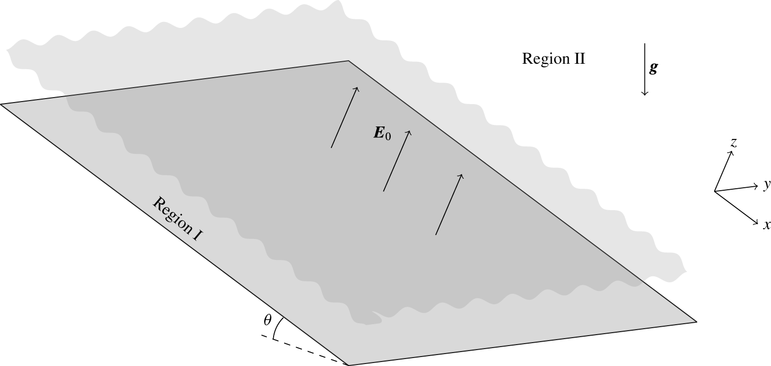
Figure 1. Schematic of the problem.
Consider a Newtonian fluid with constant density
 $\unicode[STIX]{x1D70C}$
, dynamic viscosity
$\unicode[STIX]{x1D70C}$
, dynamic viscosity
 $\unicode[STIX]{x1D707}$
and kinematic viscosity
$\unicode[STIX]{x1D707}$
and kinematic viscosity
 $\unicode[STIX]{x1D708}$
, flowing under gravity on the surface of a flat infinite two-dimensional substrate inclined at a non-zero angle
$\unicode[STIX]{x1D708}$
, flowing under gravity on the surface of a flat infinite two-dimensional substrate inclined at a non-zero angle
 $\unicode[STIX]{x1D703}$
to the horizontal. We use coordinates
$\unicode[STIX]{x1D703}$
to the horizontal. We use coordinates
 $(x,y,z)$
fixed in the plane as shown in figure 1, with
$(x,y,z)$
fixed in the plane as shown in figure 1, with
 $x$
directed down the slope in the streamwise direction,
$x$
directed down the slope in the streamwise direction,
 $y$
in the spanwise direction and
$y$
in the spanwise direction and
 $z$
perpendicular to the substrate. Note that as
$z$
perpendicular to the substrate. Note that as
 $\unicode[STIX]{x1D703}$
increases, the plate and axes rotate; for
$\unicode[STIX]{x1D703}$
increases, the plate and axes rotate; for
 $\unicode[STIX]{x1D703}\in (0,\unicode[STIX]{x03C0}/2)$
we have overlying films, for
$\unicode[STIX]{x1D703}\in (0,\unicode[STIX]{x03C0}/2)$
we have overlying films, for
 $\unicode[STIX]{x1D703}=\unicode[STIX]{x03C0}/2$
vertical films and for
$\unicode[STIX]{x1D703}=\unicode[STIX]{x03C0}/2$
vertical films and for
 $\unicode[STIX]{x1D703}\in (\unicode[STIX]{x03C0}/2,\unicode[STIX]{x03C0})$
hanging films are obtained. The surface tension coefficient between the liquid and the surrounding hydrodynamically passive medium is denoted by
$\unicode[STIX]{x1D703}\in (\unicode[STIX]{x03C0}/2,\unicode[STIX]{x03C0})$
hanging films are obtained. The surface tension coefficient between the liquid and the surrounding hydrodynamically passive medium is denoted by
 $\unicode[STIX]{x1D70E}$
(assumed constant), and the acceleration due to gravity is denoted by
$\unicode[STIX]{x1D70E}$
(assumed constant), and the acceleration due to gravity is denoted by
 $\boldsymbol{g}=(g\sin \unicode[STIX]{x1D703},0,-g\cos \unicode[STIX]{x1D703})$
. The local film thickness is represented by
$\boldsymbol{g}=(g\sin \unicode[STIX]{x1D703},0,-g\cos \unicode[STIX]{x1D703})$
. The local film thickness is represented by
 $h(x,y,t)$
, a function of space and time, with unperturbed thickness
$h(x,y,t)$
, a function of space and time, with unperturbed thickness
 $\ell$
. The liquid film is assumed to be a perfect conductor and the surrounding medium is taken to be a perfect dielectric with permittivity
$\ell$
. The liquid film is assumed to be a perfect conductor and the surrounding medium is taken to be a perfect dielectric with permittivity
 $\unicode[STIX]{x1D716}_{\unicode[STIX]{x1D6FC}}$
. A voltage is set up by grounding the plate at zero potential and imposing a uniform field normal to the plate far away, i.e.
$\unicode[STIX]{x1D716}_{\unicode[STIX]{x1D6FC}}$
. A voltage is set up by grounding the plate at zero potential and imposing a uniform field normal to the plate far away, i.e.
 $\boldsymbol{E}\rightarrow \boldsymbol{E}_{0}=(0,0,E_{0})$
as
$\boldsymbol{E}\rightarrow \boldsymbol{E}_{0}=(0,0,E_{0})$
as
 $z\rightarrow \infty$
, where
$z\rightarrow \infty$
, where
 $E_{0}$
is a constant. Denoting the voltage potential by
$E_{0}$
is a constant. Denoting the voltage potential by
 $V$
, it follows that in the electrostatic limit appropriate to this study, the electric field takes the form
$V$
, it follows that in the electrostatic limit appropriate to this study, the electric field takes the form
 $\boldsymbol{E}=-\unicode[STIX]{x1D735}V$
, where
$\boldsymbol{E}=-\unicode[STIX]{x1D735}V$
, where
 $\unicode[STIX]{x1D735}$
is the usual three-dimensional spatial gradient operator (this follows from Maxwell’s equations that yield
$\unicode[STIX]{x1D735}$
is the usual three-dimensional spatial gradient operator (this follows from Maxwell’s equations that yield
 $\unicode[STIX]{x1D735}\times \boldsymbol{E}=\mathbf{0}$
in this limit). Since the fluid is perfectly conducting, the voltage potential is zero at the fluid interface. The liquid layer and surrounding medium are denoted by Regions I and II, respectively. The fluid in Region I is governed by the incompressible Navier–Stokes equations
$\unicode[STIX]{x1D735}\times \boldsymbol{E}=\mathbf{0}$
in this limit). Since the fluid is perfectly conducting, the voltage potential is zero at the fluid interface. The liquid layer and surrounding medium are denoted by Regions I and II, respectively. The fluid in Region I is governed by the incompressible Navier–Stokes equations
 $$\begin{eqnarray}\displaystyle \boldsymbol{u}_{t}+(\boldsymbol{u}\boldsymbol{\cdot }\unicode[STIX]{x1D735})\boldsymbol{u} & = & \displaystyle -\frac{1}{\unicode[STIX]{x1D70C}}\unicode[STIX]{x1D735}p+\unicode[STIX]{x1D708}\unicode[STIX]{x1D6FB}^{2}\boldsymbol{u}+\boldsymbol{g},\end{eqnarray}$$
 $$\begin{eqnarray}\displaystyle \unicode[STIX]{x1D735}\boldsymbol{\cdot }\boldsymbol{u} & = & \displaystyle 0,\end{eqnarray}$$
 $\boldsymbol{u}=(u,v,w)$
is the velocity field,
$\boldsymbol{u}=(u,v,w)$
is the velocity field,
 $p$
is the pressure and
$p$
is the pressure and
 $\unicode[STIX]{x1D6FB}^{2}=\unicode[STIX]{x1D735}\boldsymbol{\cdot }\unicode[STIX]{x1D735}$
. Since
$\unicode[STIX]{x1D6FB}^{2}=\unicode[STIX]{x1D735}\boldsymbol{\cdot }\unicode[STIX]{x1D735}$
. Since
 $\boldsymbol{E}=-\unicode[STIX]{x1D735}V$
, and in addition Gauss’ law states that
$\boldsymbol{E}=-\unicode[STIX]{x1D735}V$
, and in addition Gauss’ law states that
 $\unicode[STIX]{x1D735}\boldsymbol{\cdot }(\unicode[STIX]{x1D716}_{\unicode[STIX]{x1D6FC}}\boldsymbol{E})=0$
(we assume that there are no volume charges in Region II), it follows that
$\unicode[STIX]{x1D735}\boldsymbol{\cdot }(\unicode[STIX]{x1D716}_{\unicode[STIX]{x1D6FC}}\boldsymbol{E})=0$
(we assume that there are no volume charges in Region II), it follows that
 $V$
satisfies Laplace’s equation in Region II,
$V$
satisfies Laplace’s equation in Region II,  $$\begin{eqnarray}\unicode[STIX]{x1D6FB}^{2}V=0,\end{eqnarray}$$
subject to the conditions
 $$\begin{eqnarray}\displaystyle V=0\quad \text{at}\;z=h(x,y,t),\quad \unicode[STIX]{x1D735}V\rightarrow -\boldsymbol{E}_{0}\quad \text{as}\;z\rightarrow \infty . & & \displaystyle\end{eqnarray}$$
For the fluid, we have no-slip conditions at the solid substrate surface,
 $\boldsymbol{u}|_{z=0}=\mathbf{0}$
, the kinematic condition
$\boldsymbol{u}|_{z=0}=\mathbf{0}$
, the kinematic condition
 $$\begin{eqnarray}w=h_{t}+uh_{x}+vh_{y}\quad \text{at}\;z=h(x,y,t),\end{eqnarray}$$
and a balance of stresses at the interface as detailed next. Any point on the interface at time
 $t$
has position vector
$t$
has position vector
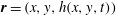 $\boldsymbol{r}=(x,y,h(x,y,t))$
. The contravariant base vectors
$\boldsymbol{r}=(x,y,h(x,y,t))$
. The contravariant base vectors
 $\boldsymbol{t}_{1},\boldsymbol{t}_{2}$
, and unit normal
$\boldsymbol{t}_{1},\boldsymbol{t}_{2}$
, and unit normal
 $\boldsymbol{n}$
are defined by
$\boldsymbol{n}$
are defined by
 $$\begin{eqnarray}\boldsymbol{t}_{1}=\frac{\unicode[STIX]{x2202}\boldsymbol{r}}{\unicode[STIX]{x2202}x}=\left(\begin{array}{@{}c@{}}1\\ 0\\ h_{x}\end{array}\right),\quad \boldsymbol{t}_{2}=\frac{\unicode[STIX]{x2202}\boldsymbol{r}}{\unicode[STIX]{x2202}y}=\left(\begin{array}{@{}c@{}}0\\ 1\\ h_{y}\end{array}\right),\quad \boldsymbol{n}=\frac{\boldsymbol{t}_{1}\times \boldsymbol{t}_{2}}{\sqrt{K}}=\frac{1}{\sqrt{K}}\left(\begin{array}{@{}c@{}}-h_{x}\\ -h_{y}\\ 1\end{array}\right),\end{eqnarray}$$
where
 $K=1+h_{x}^{2}+h_{y}^{2}$
. Since the voltage potential is constant on the interface,
$K=1+h_{x}^{2}+h_{y}^{2}$
. Since the voltage potential is constant on the interface,
 $\unicode[STIX]{x1D735}V\boldsymbol{\cdot }\boldsymbol{t}_{1}=0$
and
$\unicode[STIX]{x1D735}V\boldsymbol{\cdot }\boldsymbol{t}_{1}=0$
and
 $\unicode[STIX]{x1D735}V\boldsymbol{\cdot }\boldsymbol{t}_{2}=0$
, which written out in full are
$\unicode[STIX]{x1D735}V\boldsymbol{\cdot }\boldsymbol{t}_{2}=0$
, which written out in full are
 $$\begin{eqnarray}\displaystyle V_{x}+h_{x}V_{z}=0,\quad V_{y}+h_{y}V_{z}=0, & & \displaystyle\end{eqnarray}$$
where it is understood that all functions are evaluated at
 $z=h(x,y,t)$
. The stress tensors in Regions I and II have components
$z=h(x,y,t)$
. The stress tensors in Regions I and II have components
 $$\begin{eqnarray}\unicode[STIX]{x1D64F}_{jk}^{\text{I}}=\unicode[STIX]{x1D707}\left(\frac{\unicode[STIX]{x2202}u_{k}}{\unicode[STIX]{x2202}x_{j}}+\frac{\unicode[STIX]{x2202}u_{j}}{\unicode[STIX]{x2202}x_{k}}\right)-p\unicode[STIX]{x1D6FF}_{jk},\quad \unicode[STIX]{x1D64F}_{jk}^{\text{II}}=\unicode[STIX]{x1D716}_{\unicode[STIX]{x1D6FC}}\left(\frac{\unicode[STIX]{x2202}V}{\unicode[STIX]{x2202}x_{j}}\frac{\unicode[STIX]{x2202}V}{\unicode[STIX]{x2202}x_{k}}-\frac{1}{2}|\unicode[STIX]{x1D735}V|^{2}\unicode[STIX]{x1D6FF}_{jk}\right)-p_{\mathit{atm}}\unicode[STIX]{x1D6FF}_{jk},\end{eqnarray}$$
respectively, where
 $p_{\mathit{atm}}$
is the atmospheric pressure in Region II and we have employed the usual subscript notation for the coordinate system and velocity components. We balance the stresses in the tangential and normal directions at the interface,
$p_{\mathit{atm}}$
is the atmospheric pressure in Region II and we have employed the usual subscript notation for the coordinate system and velocity components. We balance the stresses in the tangential and normal directions at the interface,
 $$\begin{eqnarray}\displaystyle [(\unicode[STIX]{x1D64F}^{i}\boldsymbol{n})\boldsymbol{\cdot }\boldsymbol{t}_{1}]_{\text{II}}^{\text{I}}=0,\quad [(\unicode[STIX]{x1D64F}^{i}\boldsymbol{n})\boldsymbol{\cdot }\boldsymbol{t}_{2}]_{\text{II}}^{\text{I}}=0, & & \displaystyle\end{eqnarray}$$
 $$\begin{eqnarray}\displaystyle [(\unicode[STIX]{x1D64F}^{i}\boldsymbol{n})\boldsymbol{\cdot }\boldsymbol{n}]_{\text{II}}^{\text{I}}=\unicode[STIX]{x1D70E}\frac{(1+h_{x}^{2})h_{yy}-2h_{x}h_{y}h_{xy}+(1+h_{y}^{2})h_{xx}}{K^{3/2}}, & & \displaystyle\end{eqnarray}$$
where the jump notation
 $[\cdot ]_{\text{II}}^{\text{I}}=(\cdot )_{\text{I}}-(\cdot )_{\text{II}}$
has been introduced and the term multiplying
$[\cdot ]_{\text{II}}^{\text{I}}=(\cdot )_{\text{I}}-(\cdot )_{\text{II}}$
has been introduced and the term multiplying
 $\unicode[STIX]{x1D70E}$
in (2.8c
) is the curvature of the interface. Using (2.6a
), the tangential stress balance in the
$\unicode[STIX]{x1D70E}$
in (2.8c
) is the curvature of the interface. Using (2.6a
), the tangential stress balance in the
 $\boldsymbol{t}_{1}$
direction (2.8a
) becomes
$\boldsymbol{t}_{1}$
direction (2.8a
) becomes
 $$\begin{eqnarray}(1-h_{x}^{2})(u_{z}+w_{x})+2(w_{z}-u_{x})h_{x}-(u_{y}+v_{x})h_{y}-(v_{z}+w_{y})h_{x}h_{y}=0,\end{eqnarray}$$
and similarly using (2.6b
), the tangential stress balance in the
 $\boldsymbol{t}_{2}$
direction (2.8b
) reads
$\boldsymbol{t}_{2}$
direction (2.8b
) reads
 $$\begin{eqnarray}(1-h_{y}^{2})(v_{z}+w_{y})-(u_{y}+v_{x})h_{x}+2(w_{z}-v_{y})h_{y}-(u_{z}+w_{x})h_{x}h_{y}=0.\end{eqnarray}$$
The normal stress balance (2.8c ) written out in full becomes
 $$\begin{eqnarray}\displaystyle & & \displaystyle p_{\mathit{atm}}-p-\frac{\unicode[STIX]{x1D716}_{\unicode[STIX]{x1D6FC}}}{2}KV_{z}^{2}-\unicode[STIX]{x1D70E}\frac{(1+h_{x}^{2})h_{yy}-2h_{x}h_{y}h_{xy}+(1+h_{y}^{2})h_{xx}}{K^{3/2}}\nonumber\\ \displaystyle & & \displaystyle \quad +\,2\unicode[STIX]{x1D707}\frac{u_{x}h_{x}^{2}+(u_{y}+v_{x})h_{x}h_{y}+v_{y}h_{y}^{2}-(u_{z}+w_{x})h_{x}-(v_{z}+w_{y})h_{y}+w_{z}}{K}=0.\qquad\end{eqnarray}$$
The stress balances (2.9)–(2.11) complete the set of dimensional nonlinear interfacial conditions. The normal stress balance (2.11) is the originator of the coupling between the problems in Regions I and II. This is unique to the case of a perfectly conducting liquid film surrounded by a perfect dielectric (where one phase possesses infinite conductivity and the other zero conductivity, respectively), otherwise the electric field has contributions to the tangential stresses as in the case of the Taylor–Melcher leaky dielectric model (see for example Papageorgiou & Petropoulos Reference Papageorgiou and Petropoulos2004).
2.1 Non-dimensionalisation of equations
The exact Nusselt solution with a film of uniform thickness (Nusselt Reference Nusselt1916; Benjamin Reference Benjamin1957) can be modified to account for the electric field as done for the one-dimensional problem by Tseluiko & Papageorgiou (Reference Tseluiko and Papageorgiou2006b ) to give
 $$\begin{eqnarray}\left.\begin{array}{@{}c@{}}\overline{h}=\ell ,\quad \overline{u}={\displaystyle \frac{g\sin \unicode[STIX]{x1D703}}{2\unicode[STIX]{x1D708}}}(2\ell z-z^{2}),\quad \overline{v}=0,\quad \overline{w}=0,\\ \overline{p}=p_{\mathit{atm}}-{\displaystyle \frac{1}{2}}\unicode[STIX]{x1D716}_{\unicode[STIX]{x1D6FC}}E_{0}^{2}-\unicode[STIX]{x1D70C}g(z-\ell )\cos \unicode[STIX]{x1D703},\quad \overline{V}=E_{0}(\ell -z),\end{array}\right\}\end{eqnarray}$$
with bars denoting base states. The velocity profile is semi-parabolic in
 $z$
, and the voltage potential is linear in
$z$
, and the voltage potential is linear in
 $z$
as expected. We will non-dimensionalise velocities with the base velocity at the free surface,
$z$
as expected. We will non-dimensionalise velocities with the base velocity at the free surface,
 $U_{0}=\overline{u}|_{z=\ell }=g\ell ^{2}\sin \unicode[STIX]{x1D703}/2\unicode[STIX]{x1D708}$
, and make use of the non-dimensional parameters
$U_{0}=\overline{u}|_{z=\ell }=g\ell ^{2}\sin \unicode[STIX]{x1D703}/2\unicode[STIX]{x1D708}$
, and make use of the non-dimensional parameters
 $$\begin{eqnarray}Re=\frac{U_{0}\ell }{\unicode[STIX]{x1D708}}=\frac{g\ell ^{3}\sin \unicode[STIX]{x1D703}}{2\unicode[STIX]{x1D708}^{2}},\quad We=\frac{\unicode[STIX]{x1D716}_{\unicode[STIX]{x1D6FC}}E_{0}^{2}\ell }{2\unicode[STIX]{x1D707}U_{0}}=\frac{\unicode[STIX]{x1D716}_{\unicode[STIX]{x1D6FC}}E_{0}^{2}}{\unicode[STIX]{x1D70C}g\ell \sin \unicode[STIX]{x1D703}},\quad C=\frac{U_{0}\unicode[STIX]{x1D707}}{\unicode[STIX]{x1D70E}}=\frac{\unicode[STIX]{x1D70C}g\ell ^{2}\sin \unicode[STIX]{x1D703}}{2\unicode[STIX]{x1D70E}}.\end{eqnarray}$$
 $Re$
is the Reynolds number measuring the ratio of inertial to viscous forces,
$Re$
is the Reynolds number measuring the ratio of inertial to viscous forces,
 $We$
is the electric Weber number measuring the ratio of electrical to fluid pressures, and
$We$
is the electric Weber number measuring the ratio of electrical to fluid pressures, and
 $C$
is the capillary number measuring the ratio of surface tension to viscous forces. In order to non-dimensionalise and simplify the problem, we write
$C$
is the capillary number measuring the ratio of surface tension to viscous forces. In order to non-dimensionalise and simplify the problem, we write
 $$\begin{eqnarray}\left.\begin{array}{@{}c@{}}\displaystyle x^{\ast }=\frac{1}{\ell }x,\quad y^{\ast }=\frac{1}{\ell }y,\quad z^{\ast }=\frac{1}{\ell }z,\quad \boldsymbol{u}^{\ast }=\frac{1}{U_{0}}\boldsymbol{u},\quad t^{\ast }=\frac{U_{0}}{\ell }t,\quad h^{\ast }=\frac{1}{\ell }h,\\ \displaystyle p^{\ast }=\frac{\ell }{\unicode[STIX]{x1D707}U_{0}}\left(p-p_{\mathit{atm}}+\frac{1}{2}\unicode[STIX]{x1D716}_{\unicode[STIX]{x1D6FC}}E_{0}^{2}+\unicode[STIX]{x1D70C}gz\cos \unicode[STIX]{x1D703}\right),\quad V^{\ast }=\frac{1}{E_{0}\ell }(V+E_{0}z).\end{array}\right\}\end{eqnarray}$$
We substitute (2.14) into the equations and boundary conditions, and drop the stars. In Region I, the Navier–Stokes equations transform to
 $$\begin{eqnarray}\displaystyle Re(\boldsymbol{u}_{t}+(\boldsymbol{u}\boldsymbol{\cdot }\unicode[STIX]{x1D735})\boldsymbol{u}) & = & \displaystyle -\unicode[STIX]{x1D735}p+\unicode[STIX]{x1D6FB}^{2}\boldsymbol{u}+2\boldsymbol{e}_{x},\end{eqnarray}$$
 $$\begin{eqnarray}\displaystyle \unicode[STIX]{x1D735}\boldsymbol{\cdot }\boldsymbol{u} & = & \displaystyle 0,\end{eqnarray}$$
 $\boldsymbol{e}_{x}=(1,0,0)$
. Laplace’s equation in Region II and the no-slip and impermeability conditions are unchanged, while the far field condition for
$\boldsymbol{e}_{x}=(1,0,0)$
. Laplace’s equation in Region II and the no-slip and impermeability conditions are unchanged, while the far field condition for
 $V$
(2.3b
) becomes
$V$
(2.3b
) becomes
 $\unicode[STIX]{x1D735}V\rightarrow \mathbf{0}$
as
$\unicode[STIX]{x1D735}V\rightarrow \mathbf{0}$
as
 $z\rightarrow \infty$
. At the interface, the zero voltage potential condition (2.3a
) becomes
$z\rightarrow \infty$
. At the interface, the zero voltage potential condition (2.3a
) becomes
 $V=h$
at
$V=h$
at
 $z=h$
. The kinematic condition (2.4) and the tangential stress relations (2.9) and (2.10) are all unchanged, whereas the normal stress relation (2.11) transforms to
$z=h$
. The kinematic condition (2.4) and the tangential stress relations (2.9) and (2.10) are all unchanged, whereas the normal stress relation (2.11) transforms to  $$\begin{eqnarray}\displaystyle & & \displaystyle \frac{We}{2}+h\cot \unicode[STIX]{x1D703}-\frac{1}{2}p-\frac{We}{2}K(1-V_{z})^{2}\nonumber\\ \displaystyle & & \displaystyle \quad +\,\frac{u_{x}h_{x}^{2}+(u_{y}+v_{x})h_{x}h_{y}+v_{y}h_{y}^{2}-(u_{z}+w_{x})h_{x}-(v_{z}+w_{y})h_{y}+w_{z}}{K}\nonumber\\ \displaystyle & & \displaystyle \qquad =\frac{1}{2C}\frac{(1+h_{x}^{2})h_{yy}-2h_{x}h_{y}h_{xy}+(1+h_{y}^{2})h_{xx}}{K^{3/2}},\end{eqnarray}$$
where all variables are evaluated at
 $z=h$
. The system remains nonlinear and intractable analytically; in what follows we make progress by employing a long-wave expansion, in which we assume that the typical lengths in the
$z=h$
. The system remains nonlinear and intractable analytically; in what follows we make progress by employing a long-wave expansion, in which we assume that the typical lengths in the
 $x$
and
$x$
and
 $y$
directions are large compared to the film thickness.
$y$
directions are large compared to the film thickness.
3 Fully nonlinear long-wave evolution equations
We assume that the typical interfacial deformation wavelengths
 $\unicode[STIX]{x1D706}$
are large compared to the unperturbed thickness
$\unicode[STIX]{x1D706}$
are large compared to the unperturbed thickness
 $\ell$
, set
$\ell$
, set
 $\unicode[STIX]{x1D6FF}=\ell /\unicode[STIX]{x1D706}\ll 1$
and introduce the change of variables in Region I,
$\unicode[STIX]{x1D6FF}=\ell /\unicode[STIX]{x1D706}\ll 1$
and introduce the change of variables in Region I,
 $$\begin{eqnarray}x=\frac{1}{\unicode[STIX]{x1D6FF}}\widehat{x},\quad y=\frac{1}{\unicode[STIX]{x1D6FF}}\widehat{y},\quad t=\frac{1}{\unicode[STIX]{x1D6FF}}\widehat{t},\quad w=\unicode[STIX]{x1D6FF}\widehat{w}.\end{eqnarray}$$
For brevity, we omit the transformed Navier–Stokes equations. The no-slip and impermeability conditions are unchanged. Substitution of (3.1) into the interfacial conditions and dropping hats keeps the kinematic condition (2.4) unchanged, while the stress balances become
 $$\begin{eqnarray}(1-\unicode[STIX]{x1D6FF}^{2}h_{x}^{2})(u_{z}+\unicode[STIX]{x1D6FF}^{2}w_{x})+2\unicode[STIX]{x1D6FF}^{2}(w_{z}-u_{x})h_{x}-\unicode[STIX]{x1D6FF}^{2}(u_{y}+v_{x})h_{y}-\unicode[STIX]{x1D6FF}^{2}(v_{z}+\unicode[STIX]{x1D6FF}^{2}w_{y})h_{x}h_{y}=0,\end{eqnarray}$$
 $$\begin{eqnarray}(1-\unicode[STIX]{x1D6FF}^{2}h_{y}^{2})(v_{z}+\unicode[STIX]{x1D6FF}^{2}w_{y})-\unicode[STIX]{x1D6FF}^{2}(u_{y}+v_{x})h_{x}+2\unicode[STIX]{x1D6FF}^{2}(w_{z}-v_{y})h_{y}-\unicode[STIX]{x1D6FF}^{2}(u_{z}+\unicode[STIX]{x1D6FF}^{2}w_{x})h_{x}h_{y}=0,\end{eqnarray}$$
 $$\begin{eqnarray}\displaystyle & & \displaystyle \frac{We}{2}+h\cot \unicode[STIX]{x1D703}-\frac{1}{2}p-\frac{We}{2}K_{\unicode[STIX]{x1D6FF}}(1-V_{z})^{2}\nonumber\\ \displaystyle & & \displaystyle \quad +\,\unicode[STIX]{x1D6FF}\frac{\unicode[STIX]{x1D6FF}^{2}u_{x}h_{x}^{2}+\unicode[STIX]{x1D6FF}^{2}(u_{y}+v_{x})h_{x}h_{y}+\unicode[STIX]{x1D6FF}^{2}v_{y}h_{y}^{2}-(u_{z}+\unicode[STIX]{x1D6FF}^{2}w_{x})h_{x}-(v_{z}+\unicode[STIX]{x1D6FF}^{2}w_{y})h_{y}+w_{z}}{K_{\unicode[STIX]{x1D6FF}}}\nonumber\\ \displaystyle & & \displaystyle \qquad =\frac{\unicode[STIX]{x1D6FF}^{2}}{2C}\frac{(1+\unicode[STIX]{x1D6FF}^{2}h_{x}^{2})h_{yy}-2\unicode[STIX]{x1D6FF}^{2}h_{x}h_{y}h_{xy}+(1+\unicode[STIX]{x1D6FF}^{2}h_{y}^{2})h_{xx}}{K_{\unicode[STIX]{x1D6FF}}^{3/2}},\end{eqnarray}$$
where
 $K_{\unicode[STIX]{x1D6FF}}=\unicode[STIX]{x1D6FF}^{2}h_{x}^{2}+\unicode[STIX]{x1D6FF}^{2}h_{y}^{2}+1$
and all variables are evaluated at
$K_{\unicode[STIX]{x1D6FF}}=\unicode[STIX]{x1D6FF}^{2}h_{x}^{2}+\unicode[STIX]{x1D6FF}^{2}h_{y}^{2}+1$
and all variables are evaluated at
 $z=h$
.
$z=h$
.
The normal stress balance (3.2c
) contains the non-local contribution
 $V_{z}|_{z=h}$
, where
$V_{z}|_{z=h}$
, where
 $V$
satisfies Laplace’s equation in Region II. To calculate this, we consider a rescaled normal variable
$V$
satisfies Laplace’s equation in Region II. To calculate this, we consider a rescaled normal variable
 $\unicode[STIX]{x1D701}=\unicode[STIX]{x1D6FF}z$
in Region II, along with the same temporal and spatial rescalings (3.1a–c
) as in Region I with a view to obtain
$\unicode[STIX]{x1D701}=\unicode[STIX]{x1D6FF}z$
in Region II, along with the same temporal and spatial rescalings (3.1a–c
) as in Region I with a view to obtain
 $V_{\unicode[STIX]{x1D701}}|_{\unicode[STIX]{x1D701}=\unicode[STIX]{x1D6FF}h}$
to leading order. Introducing the asymptotic expansions
$V_{\unicode[STIX]{x1D701}}|_{\unicode[STIX]{x1D701}=\unicode[STIX]{x1D6FF}h}$
to leading order. Introducing the asymptotic expansions
 $$\begin{eqnarray}h=h_{0}+\unicode[STIX]{x1D6FF}h_{1}+\unicode[STIX]{x1D6FF}^{2}h_{2}+\cdots \,,\quad V=V_{0}+\unicode[STIX]{x1D6FF}V_{1}+\unicode[STIX]{x1D6FF}^{2}V_{2}+\cdots \,,\end{eqnarray}$$
and noting that
 $V|_{\unicode[STIX]{x1D701}=\unicode[STIX]{x1D6FF}h}=V_{0}|_{\unicode[STIX]{x1D701}=0}+O(\unicode[STIX]{x1D6FF})$
,
$V|_{\unicode[STIX]{x1D701}=\unicode[STIX]{x1D6FF}h}=V_{0}|_{\unicode[STIX]{x1D701}=0}+O(\unicode[STIX]{x1D6FF})$
,
 $V_{\unicode[STIX]{x1D701}}|_{\unicode[STIX]{x1D701}=\unicode[STIX]{x1D6FF}h}=(V_{0})_{\unicode[STIX]{x1D701}}|_{\unicode[STIX]{x1D701}=0}+O(\unicode[STIX]{x1D6FF})$
, yields the leading-order problem
$V_{\unicode[STIX]{x1D701}}|_{\unicode[STIX]{x1D701}=\unicode[STIX]{x1D6FF}h}=(V_{0})_{\unicode[STIX]{x1D701}}|_{\unicode[STIX]{x1D701}=0}+O(\unicode[STIX]{x1D6FF})$
, yields the leading-order problem
 $$\begin{eqnarray}\unicode[STIX]{x1D6FB}^{2}V_{0}=0,\quad V_{0}|_{\unicode[STIX]{x1D701}=0}=h_{0},\quad \unicode[STIX]{x1D735}V_{0}\rightarrow \mathbf{0}\quad \text{as}\;\unicode[STIX]{x1D701}\rightarrow \infty .\end{eqnarray}$$
By taking Fourier transforms in
 $x$
and
$x$
and
 $y$
and considering the resulting differential equation, it follows that
$y$
and considering the resulting differential equation, it follows that
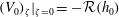 $(V_{0})_{\unicode[STIX]{x1D701}}|_{\unicode[STIX]{x1D701}=0}=-{\mathcal{R}}(h_{0})$
where
$(V_{0})_{\unicode[STIX]{x1D701}}|_{\unicode[STIX]{x1D701}=0}=-{\mathcal{R}}(h_{0})$
where
 ${\mathcal{R}}$
is a fractional Laplacian with Fourier symbol
${\mathcal{R}}$
is a fractional Laplacian with Fourier symbol
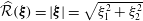 $\widehat{{\mathcal{R}}}(\unicode[STIX]{x1D743})=|\unicode[STIX]{x1D743}|=\sqrt{\unicode[STIX]{x1D709}_{1}^{2}+\unicode[STIX]{x1D709}_{2}^{2}}$
for wavenumber vector
$\widehat{{\mathcal{R}}}(\unicode[STIX]{x1D743})=|\unicode[STIX]{x1D743}|=\sqrt{\unicode[STIX]{x1D709}_{1}^{2}+\unicode[STIX]{x1D709}_{2}^{2}}$
for wavenumber vector
 $\unicode[STIX]{x1D743}=(\unicode[STIX]{x1D709}_{1},\unicode[STIX]{x1D709}_{2})$
. The common notation in the literature is
$\unicode[STIX]{x1D743}=(\unicode[STIX]{x1D709}_{1},\unicode[STIX]{x1D709}_{2})$
. The common notation in the literature is
 ${\mathcal{R}}=(-\unicode[STIX]{x1D6E5})^{1/2}$
, where
${\mathcal{R}}=(-\unicode[STIX]{x1D6E5})^{1/2}$
, where
 $\unicode[STIX]{x1D6E5}\equiv \unicode[STIX]{x2202}_{x}^{2}+\unicode[STIX]{x2202}_{y}^{2}$
is the two-dimensional Laplace operator. We have an integral representation (Córdoba & Córdoba Reference Córdoba and Córdoba2004),
$\unicode[STIX]{x1D6E5}\equiv \unicode[STIX]{x2202}_{x}^{2}+\unicode[STIX]{x2202}_{y}^{2}$
is the two-dimensional Laplace operator. We have an integral representation (Córdoba & Córdoba Reference Córdoba and Córdoba2004),
 $$\begin{eqnarray}{\mathcal{R}}(f)=\frac{1}{2\unicode[STIX]{x03C0}}\int _{\mathbb{R}^{2}}\frac{f(\boldsymbol{x})-f(\boldsymbol{x}^{\prime })}{|\boldsymbol{x}-\boldsymbol{x}^{\prime }|^{3}}\,\text{d}\boldsymbol{x}^{\prime },\end{eqnarray}$$
where
 $\boldsymbol{x}=(x,y)$
,
$\boldsymbol{x}=(x,y)$
,
 $\boldsymbol{x}^{\prime }=(x^{\prime },y^{\prime })$
, and the integral is understood in a principal value sense. Returning to the unscaled variable
$\boldsymbol{x}^{\prime }=(x^{\prime },y^{\prime })$
, and the integral is understood in a principal value sense. Returning to the unscaled variable
 $z=\unicode[STIX]{x1D701}/\unicode[STIX]{x1D6FF}$
, the non-local contribution in the normal stress balance (3.2c
) is
$z=\unicode[STIX]{x1D701}/\unicode[STIX]{x1D6FF}$
, the non-local contribution in the normal stress balance (3.2c
) is
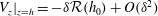 $V_{z}|_{z=h}=-\unicode[STIX]{x1D6FF}{\mathcal{R}}(h_{0})+O(\unicode[STIX]{x1D6FF}^{2})$
. It follows from (3.2c
) that in order to retain the effects of surface tension and the electric field in the leading-order dynamics, we must take the scalings
$V_{z}|_{z=h}=-\unicode[STIX]{x1D6FF}{\mathcal{R}}(h_{0})+O(\unicode[STIX]{x1D6FF}^{2})$
. It follows from (3.2c
) that in order to retain the effects of surface tension and the electric field in the leading-order dynamics, we must take the scalings
 $$\begin{eqnarray}C=\unicode[STIX]{x1D6FF}^{2}\overline{C},\quad We=\frac{\overline{We}}{\unicode[STIX]{x1D6FF}},\end{eqnarray}$$
where
 $\overline{C}$
and
$\overline{C}$
and
 $\overline{We}$
are
$\overline{We}$
are
 $O(1)$
quantities. We also assume that the Reynolds number
$O(1)$
quantities. We also assume that the Reynolds number
 $Re$
is an
$Re$
is an
 $O(1)$
quantity.
$O(1)$
quantity.
Turning to the fluid dynamics in Region I, we introduce the following asymptotic expansions
 $$\begin{eqnarray}\left.\begin{array}{@{}c@{}}\displaystyle u=u_{0}+\unicode[STIX]{x1D6FF}u_{1}+\unicode[STIX]{x1D6FF}^{2}u_{2}+\cdots \,,\quad v=v_{0}+\unicode[STIX]{x1D6FF}v_{1}+\unicode[STIX]{x1D6FF}^{2}v_{2}+\cdots \,,\\ w=w_{0}+\unicode[STIX]{x1D6FF}w_{1}+\unicode[STIX]{x1D6FF}^{2}w_{2}+\cdots \,,\quad p=p_{0}+\unicode[STIX]{x1D6FF}p_{1}+\unicode[STIX]{x1D6FF}^{2}p_{2}+\cdots \,.\end{array}\right\}\end{eqnarray}$$
The leading-order terms of the momentum equations in the streamwise and spanwise directions are
 $$\begin{eqnarray}(u_{0})_{zz}=-2,\quad (v_{0})_{zz}=0.\end{eqnarray}$$
These can be integrated to obtain
 $$\begin{eqnarray}(u_{0})_{z}=2(h_{0}-z),\quad (v_{0})_{z}=0,\end{eqnarray}$$
where we have used the leading-order terms of the tangential stress balances (3.2a
) and (3.2b
), which are
 $(u_{0})_{z}|_{z=h_{0}}=0$
and
$(u_{0})_{z}|_{z=h_{0}}=0$
and
 $(v_{0})_{z}|_{z=h_{0}}=0$
, respectively. One more integration, use of no-slip and the leading-order continuity equation provides the leading-order flow field
$(v_{0})_{z}|_{z=h_{0}}=0$
, respectively. One more integration, use of no-slip and the leading-order continuity equation provides the leading-order flow field
 $$\begin{eqnarray}u_{0}=(2h_{0}-z)z,\quad v_{0}=0,\quad w_{0}=-z^{2}(h_{0})_{x}.\end{eqnarray}$$
To leading order, the kinematic equation (2.4) is
 $$\begin{eqnarray}(h_{0})_{t}+u_{0}(h_{0})_{x}+v_{0}(h_{0})_{y}-w_{0}=0\quad \text{at}\;z=h_{0}(x,y,t).\end{eqnarray}$$
Substituting (3.10) into this yields
 $$\begin{eqnarray}(h_{0})_{t}+2h_{0}^{2}(h_{0})_{x}=0.\end{eqnarray}$$
We need to regularise this equation by adding higher-order terms since its solutions encounter infinite slope singularities at finite times and the long-wave expansion breaks down. To leading order, the
 $z$
-momentum equation implies that
$z$
-momentum equation implies that
 $p_{0}$
is independent of
$p_{0}$
is independent of
 $z$
, and then using the normal stress balance (3.2c
) gives
$z$
, and then using the normal stress balance (3.2c
) gives
 $$\begin{eqnarray}p_{0}=2\left[h_{0}\cot \unicode[STIX]{x1D703}-\overline{We}{\mathcal{R}}(h_{0})-\frac{1}{2\overline{C}}\unicode[STIX]{x0394}h_{0}\right].\end{eqnarray}$$
We proceed as before, but now collect
 $O(\unicode[STIX]{x1D6FF})$
terms in the governing equations and boundary conditions. The first-order velocities
$O(\unicode[STIX]{x1D6FF})$
terms in the governing equations and boundary conditions. The first-order velocities
 $u_{1}$
,
$u_{1}$
,
 $v_{1}$
and
$v_{1}$
and
 $w_{1}$
can be found analytically by integration of the second-order momentum equations (and using tangential stresses, no-slip and the continuity equation). For completeness, these are
$w_{1}$
can be found analytically by integration of the second-order momentum equations (and using tangential stresses, no-slip and the continuity equation). For completeness, these are
 $$\begin{eqnarray}u_{1}=\left[\frac{1}{2}z^{2}-zh_{0}\right](p_{0})_{x}+Re\left[\frac{1}{6}z^{4}h_{0}-\frac{2}{3}z^{3}h_{0}^{2}+\frac{4}{3}zh_{0}^{4}\right](h_{0})_{x}+2zh_{1},\end{eqnarray}$$
 $$\begin{eqnarray}\displaystyle v_{1}=\left[\frac{1}{2}z^{2}-zh_{0}\right](p_{0})_{y},\quad w_{1}=-\int _{0}^{z}(u_{1})_{x}+(v_{1})_{y}\,\text{d}z^{\prime }. & & \displaystyle\end{eqnarray}$$
The second-order contribution to the kinematic condition (2.4) is found to be
 $$\begin{eqnarray}(h_{1})_{t}+u_{1}(h_{0})_{x}+v_{1}(h_{0})_{y}-w_{1}+2h_{0}h_{1}(h_{0})_{x}+h_{0}^{2}(h_{1})_{x}=0\quad \text{at}\;z=h_{0}(x,y,t),\end{eqnarray}$$
where Taylor expansions about
 $z=h_{0}$
have been used. Substitution of the first-order velocities (3.14) gives the time evolution of
$z=h_{0}$
have been used. Substitution of the first-order velocities (3.14) gives the time evolution of
 $h_{1}$
,
$h_{1}$
,
 $$\begin{eqnarray}(h_{1})_{t}+\left[2h_{0}^{2}h_{1}+\frac{8Re}{15}h_{0}^{6}(h_{0})_{x}-\frac{1}{3}h_{0}^{3}(p_{0})_{x}\right]_{x}+\left[-\frac{1}{3}h_{0}^{3}(p_{0})_{y}\right]_{y}=0.\end{eqnarray}$$
A regularised Benney equation for
 $H=h_{0}+\unicode[STIX]{x1D6FF}h_{1}$
, with errors of
$H=h_{0}+\unicode[STIX]{x1D6FF}h_{1}$
, with errors of
 $O(\unicode[STIX]{x1D6FF}^{2})$
, is found by adding
$O(\unicode[STIX]{x1D6FF}^{2})$
, is found by adding
 $\unicode[STIX]{x1D6FF}$
times equation (3.16) to (3.12), this is
$\unicode[STIX]{x1D6FF}$
times equation (3.16) to (3.12), this is
 $$\begin{eqnarray}H_{t}+\unicode[STIX]{x1D735}\boldsymbol{\cdot }\left[\left(\frac{2}{3}H^{3}+\frac{8Re}{15}\unicode[STIX]{x1D6FF}H^{6}H_{x}\right)\boldsymbol{e}_{x}-\frac{2}{3}\unicode[STIX]{x1D6FF}H^{3}\unicode[STIX]{x1D735}\left(H\cot \unicode[STIX]{x1D703}-\overline{We}{\mathcal{R}}(H)-\frac{1}{2\overline{C}}\unicode[STIX]{x0394}H\right)\right]=0,\end{eqnarray}$$
where we have redefined
 $\unicode[STIX]{x1D735}=(\unicode[STIX]{x2202}_{x},\unicode[STIX]{x2202}_{y})$
and
$\unicode[STIX]{x1D735}=(\unicode[STIX]{x2202}_{x},\unicode[STIX]{x2202}_{y})$
and
 $\boldsymbol{e}_{x}=(1,0)$
. As noted by Tseluiko & Papageorgiou (Reference Tseluiko and Papageorgiou2006b
) for the one-dimensional analogue of (3.17), solutions may not exist for all time for some parameters, and finite-time blow-ups are observed in numerical simulations (Pumir, Manneville & Pomeau Reference Pumir, Manneville and Pomeau1983; Rosenau, Oron & Hyman Reference Rosenau, Oron and Hyman1992). Due to such global existence difficulties, we proceed by studying the weakly nonlinear evolution of a sufficiently small perturbation to the uniform state. The above procedure was also carried out to the next order in
$\boldsymbol{e}_{x}=(1,0)$
. As noted by Tseluiko & Papageorgiou (Reference Tseluiko and Papageorgiou2006b
) for the one-dimensional analogue of (3.17), solutions may not exist for all time for some parameters, and finite-time blow-ups are observed in numerical simulations (Pumir, Manneville & Pomeau Reference Pumir, Manneville and Pomeau1983; Rosenau, Oron & Hyman Reference Rosenau, Oron and Hyman1992). Due to such global existence difficulties, we proceed by studying the weakly nonlinear evolution of a sufficiently small perturbation to the uniform state. The above procedure was also carried out to the next order in
 $\unicode[STIX]{x1D6FF}$
to calculate a Benney equation with errors of
$\unicode[STIX]{x1D6FF}$
to calculate a Benney equation with errors of
 $O(\unicode[STIX]{x1D6FF}^{3})$
; this is required to retain dispersive effects. This equation is currently under investigation and findings will be reported in future work.
$O(\unicode[STIX]{x1D6FF}^{3})$
; this is required to retain dispersive effects. This equation is currently under investigation and findings will be reported in future work.
4 A multidimensional non-local Kuramoto–Sivashinsky equation
4.1 Weakly nonlinear evolution
We substitute
 $H=1+\unicode[STIX]{x1D6FF}\unicode[STIX]{x1D702}$
into (3.17) where
$H=1+\unicode[STIX]{x1D6FF}\unicode[STIX]{x1D702}$
into (3.17) where
 $\unicode[STIX]{x1D702}=O(1)$
, and also assume that
$\unicode[STIX]{x1D702}=O(1)$
, and also assume that
 $\cot \unicode[STIX]{x1D703}=O(1)$
(for the one-dimensional equation, see Tseluiko & Papageorgiou Reference Tseluiko and Papageorgiou2006b
). Moving to a slow time scale and performing a Galilean transformation with the rescaling
$\cot \unicode[STIX]{x1D703}=O(1)$
(for the one-dimensional equation, see Tseluiko & Papageorgiou Reference Tseluiko and Papageorgiou2006b
). Moving to a slow time scale and performing a Galilean transformation with the rescaling
 $$\begin{eqnarray}\overline{t}=4\unicode[STIX]{x1D6FF}t,\quad \overline{x}=x-2t,\end{eqnarray}$$
and then dropping bars gives the leading-order equation
 $$\begin{eqnarray}\unicode[STIX]{x1D702}_{t}+\unicode[STIX]{x1D702}\unicode[STIX]{x1D702}_{x}+(\unicode[STIX]{x1D6FD}^{\ast }-\unicode[STIX]{x1D705})\unicode[STIX]{x1D702}_{xx}-\unicode[STIX]{x1D705}\unicode[STIX]{x1D702}_{yy}+\unicode[STIX]{x1D6FE}^{\ast }\unicode[STIX]{x0394}{\mathcal{R}}(\unicode[STIX]{x1D702})+\unicode[STIX]{x1D707}\unicode[STIX]{x1D6E5}^{2}\unicode[STIX]{x1D702}=0.\end{eqnarray}$$
Here the
 $O(1)$
parameters are
$O(1)$
parameters are
 $$\begin{eqnarray}\unicode[STIX]{x1D6FD}^{\ast }=\frac{2Re}{15},\quad \unicode[STIX]{x1D705}=\frac{1}{6}\cot \unicode[STIX]{x1D703},\quad \unicode[STIX]{x1D6FE}^{\ast }=\frac{\overline{We}}{6},\quad \unicode[STIX]{x1D707}=\frac{1}{12\overline{C}},\end{eqnarray}$$
and
 $\unicode[STIX]{x1D6E5}\equiv \unicode[STIX]{x2202}_{x}^{2}+\unicode[STIX]{x2202}_{y}^{2}$
is the two-dimensional Laplace operator as before. The spatial average of a solution is a conserved quantity for (4.2) – this is set to zero as the interfacial perturbation should conserve the fluid mass. It is clear from our previous rescalings that
$\unicode[STIX]{x1D6E5}\equiv \unicode[STIX]{x2202}_{x}^{2}+\unicode[STIX]{x2202}_{y}^{2}$
is the two-dimensional Laplace operator as before. The spatial average of a solution is a conserved quantity for (4.2) – this is set to zero as the interfacial perturbation should conserve the fluid mass. It is clear from our previous rescalings that
 $\unicode[STIX]{x1D6FD}^{\ast },\unicode[STIX]{x1D707}>0$
,
$\unicode[STIX]{x1D6FD}^{\ast },\unicode[STIX]{x1D707}>0$
,
 $\unicode[STIX]{x1D6FE}^{\ast }\geqslant 0$
, and that
$\unicode[STIX]{x1D6FE}^{\ast }\geqslant 0$
, and that
 $\unicode[STIX]{x1D705}>0$
,
$\unicode[STIX]{x1D705}>0$
,
 $\unicode[STIX]{x1D705}=0$
, or
$\unicode[STIX]{x1D705}=0$
, or
 $\unicode[STIX]{x1D705}<0$
depending on whether the film is overlying, vertical or hanging, respectively. The choice of
$\unicode[STIX]{x1D705}<0$
depending on whether the film is overlying, vertical or hanging, respectively. The choice of
 $\unicode[STIX]{x1D6FD}^{\ast }=\unicode[STIX]{x1D705}$
corresponds to taking the critical Reynolds number for the flow, above which the flow becomes unstable to long waves (in the absence of a field). Note that if the electric field is removed and we also consider a vertical substrate, setting
$\unicode[STIX]{x1D6FD}^{\ast }=\unicode[STIX]{x1D705}$
corresponds to taking the critical Reynolds number for the flow, above which the flow becomes unstable to long waves (in the absence of a field). Note that if the electric field is removed and we also consider a vertical substrate, setting
 $\unicode[STIX]{x1D6FE}^{\ast }=0$
and
$\unicode[STIX]{x1D6FE}^{\ast }=0$
and
 $\unicode[STIX]{x1D705}=0$
in (4.2), then after rescaling, the two-dimensional Kuramoto–Sivashinsky equation (1.4) obtained by Nepomnyashchy (Reference Nepomnyashchy1974a
,Reference Nepomnyashchy
b
) is recovered. The operator corresponding to the linear part of (4.2),
$\unicode[STIX]{x1D705}=0$
in (4.2), then after rescaling, the two-dimensional Kuramoto–Sivashinsky equation (1.4) obtained by Nepomnyashchy (Reference Nepomnyashchy1974a
,Reference Nepomnyashchy
b
) is recovered. The operator corresponding to the linear part of (4.2),
 $$\begin{eqnarray}{\mathcal{L}}=(\unicode[STIX]{x1D6FD}^{\ast }-\unicode[STIX]{x1D705})\unicode[STIX]{x2202}_{xx}-\unicode[STIX]{x1D705}\unicode[STIX]{x2202}_{yy}+\unicode[STIX]{x1D6FE}^{\ast }\unicode[STIX]{x0394}{\mathcal{R}}+\unicode[STIX]{x1D707}\unicode[STIX]{x1D6E5}^{2},\end{eqnarray}$$
has Fourier symbol
 $$\begin{eqnarray}\widehat{{\mathcal{L}}}(\unicode[STIX]{x1D743})=-(\unicode[STIX]{x1D6FD}^{\ast }-\unicode[STIX]{x1D705})\unicode[STIX]{x1D709}_{1}^{2}+\unicode[STIX]{x1D705}\unicode[STIX]{x1D709}_{2}^{2}-\unicode[STIX]{x1D6FE}^{\ast }(\unicode[STIX]{x1D709}_{1}^{2}+\unicode[STIX]{x1D709}_{2}^{2})^{3/2}+\unicode[STIX]{x1D707}(\unicode[STIX]{x1D709}_{1}^{2}+\unicode[STIX]{x1D709}_{2}^{2})^{2}\end{eqnarray}$$
for wavenumber vector
 $\unicode[STIX]{x1D743}=(\unicode[STIX]{x1D709}_{1},\unicode[STIX]{x1D709}_{2})$
. If we consider hanging films with
$\unicode[STIX]{x1D743}=(\unicode[STIX]{x1D709}_{1},\unicode[STIX]{x1D709}_{2})$
. If we consider hanging films with
 $\unicode[STIX]{x1D705}<0$
, then it is clear that there are linearly unstable
$\unicode[STIX]{x1D705}<0$
, then it is clear that there are linearly unstable
 $y$
-modes (Fourier modes which are purely transverse). Even for overlying films with non-zero values of
$y$
-modes (Fourier modes which are purely transverse). Even for overlying films with non-zero values of
 $\unicode[STIX]{x1D6FE}^{\ast }$
and sufficiently small values of the product
$\unicode[STIX]{x1D6FE}^{\ast }$
and sufficiently small values of the product
 $\unicode[STIX]{x1D705}\unicode[STIX]{x1D707}$
, a band of low
$\unicode[STIX]{x1D705}\unicode[STIX]{x1D707}$
, a band of low
 $y$
-modes are linearly unstable due to the non-local term corresponding to the electric field. Due to the form of the nonlinearity in (4.2), there is no energy transfer between
$y$
-modes are linearly unstable due to the non-local term corresponding to the electric field. Due to the form of the nonlinearity in (4.2), there is no energy transfer between
 $y$
-modes. Thus, if a
$y$
-modes. Thus, if a
 $y$
-mode is linearly unstable, then it will grow exponentially without bound and the problem is ill-posed in this sense. There is no control over these transverse instabilities, and the weakly nonlinear analysis cannot be modified to overcome this issue. Since the case of
$y$
-mode is linearly unstable, then it will grow exponentially without bound and the problem is ill-posed in this sense. There is no control over these transverse instabilities, and the weakly nonlinear analysis cannot be modified to overcome this issue. Since the case of
 $\unicode[STIX]{x1D6FE}^{\ast }=0$
is not of particular interest, we are forced to restrict to overlying films with
$\unicode[STIX]{x1D6FE}^{\ast }=0$
is not of particular interest, we are forced to restrict to overlying films with
 $\unicode[STIX]{x1D705}>0$
by taking
$\unicode[STIX]{x1D705}>0$
by taking
 $\unicode[STIX]{x1D703}\in (0,\unicode[STIX]{x03C0}/2)$
(if
$\unicode[STIX]{x1D703}\in (0,\unicode[STIX]{x03C0}/2)$
(if
 $\unicode[STIX]{x1D705}=0$
, then for any
$\unicode[STIX]{x1D705}=0$
, then for any
 $\unicode[STIX]{x1D6FE}^{\ast }>0$
there are unstable transverse modes); in the remainder of this paper we study overlying films only. We rescale (4.2) with
$\unicode[STIX]{x1D6FE}^{\ast }>0$
there are unstable transverse modes); in the remainder of this paper we study overlying films only. We rescale (4.2) with
 $$\begin{eqnarray}\overline{t}=\frac{\unicode[STIX]{x1D705}^{2}}{\unicode[STIX]{x1D707}}t,\quad \overline{x}=\frac{\unicode[STIX]{x1D705}^{1/2}}{\unicode[STIX]{x1D707}^{1/2}}x,\quad \overline{y}=\frac{\unicode[STIX]{x1D705}^{1/2}}{\unicode[STIX]{x1D707}^{1/2}}y,\quad \overline{\unicode[STIX]{x1D702}}=\frac{\unicode[STIX]{x1D707}^{1/2}}{\unicode[STIX]{x1D705}^{3/2}}\unicode[STIX]{x1D702},\end{eqnarray}$$
and once again drop the bars to obtain the following canonical equation for overlying electrified films,
 $$\begin{eqnarray}\unicode[STIX]{x1D702}_{t}+\unicode[STIX]{x1D702}\unicode[STIX]{x1D702}_{x}+(\unicode[STIX]{x1D6FD}-1)\unicode[STIX]{x1D702}_{xx}-\unicode[STIX]{x1D702}_{yy}+\unicode[STIX]{x1D6FE}\unicode[STIX]{x0394}{\mathcal{R}}(\unicode[STIX]{x1D702})+\unicode[STIX]{x1D6E5}^{2}\unicode[STIX]{x1D702}=0.\end{eqnarray}$$
The parameters
 $\unicode[STIX]{x1D6FD}>0$
,
$\unicode[STIX]{x1D6FD}>0$
,
 $\unicode[STIX]{x1D6FE}\geqslant 0$
are defined by
$\unicode[STIX]{x1D6FE}\geqslant 0$
are defined by
 $$\begin{eqnarray}\unicode[STIX]{x1D6FD}=\frac{\unicode[STIX]{x1D6FD}^{\ast }}{\unicode[STIX]{x1D705}},\quad \unicode[STIX]{x1D6FE}=\frac{\unicode[STIX]{x1D6FE}^{\ast }}{\unicode[STIX]{x1D705}^{1/2}\unicode[STIX]{x1D707}^{1/2}},\end{eqnarray}$$
where
 $\unicode[STIX]{x1D6FD}=1$
corresponds to the critical Reynolds number flow. To prevent unbounded growth of solutions, equation (4.7) is studied under certain restrictions on
$\unicode[STIX]{x1D6FD}=1$
corresponds to the critical Reynolds number flow. To prevent unbounded growth of solutions, equation (4.7) is studied under certain restrictions on
 $\unicode[STIX]{x1D6FE}$
and domain choice (both
$\unicode[STIX]{x1D6FE}$
and domain choice (both
 $\unicode[STIX]{x1D6FE}$
and the domain dimensions affect the unstable spectrum as we see below). We proceed with
$\unicode[STIX]{x1D6FE}$
and the domain dimensions affect the unstable spectrum as we see below). We proceed with
 $Q$
-periodic domains (where
$Q$
-periodic domains (where
 $Q=[0,L_{1}]\times [0,L_{2}]$
) for which there are no unstable
$Q=[0,L_{1}]\times [0,L_{2}]$
) for which there are no unstable
 $y$
-modes for the choices of
$y$
-modes for the choices of
 $L_{1}$
and
$L_{1}$
and
 $L_{2}$
, leaving us only with a restriction on
$L_{2}$
, leaving us only with a restriction on
 $\unicode[STIX]{x1D6FE}$
. In what follows, we perform a linear stability analysis expanding on the above discussion to determine this condition. In the two-dimensional analogue of our problem where the interface dynamics is governed by (1.1), all instabilities are controlled by the energy transfer due to the nonlinear term. The potential for unbounded growth of transverse modes caused by strong electric fields or hanging arrangements is unique to the full three-dimensional problem.
$\unicode[STIX]{x1D6FE}$
. In what follows, we perform a linear stability analysis expanding on the above discussion to determine this condition. In the two-dimensional analogue of our problem where the interface dynamics is governed by (1.1), all instabilities are controlled by the energy transfer due to the nonlinear term. The potential for unbounded growth of transverse modes caused by strong electric fields or hanging arrangements is unique to the full three-dimensional problem.
4.2 Linear stability analysis
We linearise (4.7) about
 $\unicode[STIX]{x1D702}=0$
to obtain
$\unicode[STIX]{x1D702}=0$
to obtain
 $$\begin{eqnarray}\unicode[STIX]{x1D702}_{t}+(\unicode[STIX]{x1D6FD}-1)\unicode[STIX]{x1D702}_{xx}-\unicode[STIX]{x1D702}_{yy}+\unicode[STIX]{x1D6FE}\unicode[STIX]{x0394}{\mathcal{R}}(\unicode[STIX]{x1D702})+\unicode[STIX]{x1D6E5}^{2}\unicode[STIX]{x1D702}=0,\end{eqnarray}$$
and look for solutions of the form
 $$\begin{eqnarray}\unicode[STIX]{x1D702}(\boldsymbol{x},t)=\mathop{\sum }_{\boldsymbol{k}\in \mathbb{Z}^{2}}A_{\boldsymbol{k}}\text{e}^{\text{i}\tilde{\boldsymbol{k}}\boldsymbol{\cdot }\boldsymbol{x}+s(\tilde{\boldsymbol{k}})t},\end{eqnarray}$$
where
 $s(\tilde{\boldsymbol{k}})$
is the growth rate,
$s(\tilde{\boldsymbol{k}})$
is the growth rate,
 $A_{\boldsymbol{k}}$
are constants, and
$A_{\boldsymbol{k}}$
are constants, and
 $\tilde{\boldsymbol{k}}$
has components
$\tilde{\boldsymbol{k}}$
has components
 $$\begin{eqnarray}\tilde{k}_{1}=\frac{2\unicode[STIX]{x03C0}}{L_{1}}k_{1},\quad \tilde{k}_{2}=\frac{2\unicode[STIX]{x03C0}}{L_{2}}k_{2},\end{eqnarray}$$
for
 $\boldsymbol{k}\in \mathbb{Z}^{2}$
(we use this notation to distinguish the wavenumber vectors
$\boldsymbol{k}\in \mathbb{Z}^{2}$
(we use this notation to distinguish the wavenumber vectors
 $\tilde{\boldsymbol{k}}$
in the discrete spectrum from the general wavenumber vectors
$\tilde{\boldsymbol{k}}$
in the discrete spectrum from the general wavenumber vectors
 $\unicode[STIX]{x1D743}\in \mathbb{R}^{2}$
for a continuous spectrum). Using the Fourier symbol of the operator
$\unicode[STIX]{x1D743}\in \mathbb{R}^{2}$
for a continuous spectrum). Using the Fourier symbol of the operator
 ${\mathcal{R}}$
, the dispersion relation follows readily,
${\mathcal{R}}$
, the dispersion relation follows readily,
 $$\begin{eqnarray}s(\tilde{k}_{1},\tilde{k}_{2})=(\unicode[STIX]{x1D6FD}-1)\tilde{k}_{1}^{2}-\tilde{k}_{2}^{2}+\unicode[STIX]{x1D6FE}(\tilde{k}_{1}^{2}+\tilde{k}_{2}^{2})^{3/2}-(\tilde{k}_{1}^{2}+\tilde{k}_{2}^{2})^{2}.\end{eqnarray}$$
Instead of working with domain dimensions
 $L_{1}$
and
$L_{1}$
and
 $L_{2}$
, we introduce the parameters
$L_{2}$
, we introduce the parameters
 $$\begin{eqnarray}\unicode[STIX]{x1D708}_{1}=\left(\frac{2\unicode[STIX]{x03C0}}{L_{1}}\right)^{2},\quad \unicode[STIX]{x1D708}_{2}=\left(\frac{2\unicode[STIX]{x03C0}}{L_{2}}\right)^{2},\end{eqnarray}$$
which simplifies (4.12) to
 $$\begin{eqnarray}s(k_{1},k_{2})=(\unicode[STIX]{x1D6FD}-1)\unicode[STIX]{x1D708}_{1}k_{1}^{2}-\unicode[STIX]{x1D708}_{2}k_{2}^{2}+\unicode[STIX]{x1D6FE}(\unicode[STIX]{x1D708}_{1}k_{1}^{2}+\unicode[STIX]{x1D708}_{2}k_{2}^{2})^{3/2}-(\unicode[STIX]{x1D708}_{1}k_{1}^{2}+\unicode[STIX]{x1D708}_{2}k_{2}^{2})^{2}.\end{eqnarray}$$
Instability is found when
 $s(k_{1},k_{2})>0$
(note that
$s(k_{1},k_{2})>0$
(note that
 $s$
is real) and neutral stability curves for a given mode
$s$
is real) and neutral stability curves for a given mode
 $(k_{1},k_{2})$
in the
$(k_{1},k_{2})$
in the
 $\unicode[STIX]{x1D708}_{1}$
–
$\unicode[STIX]{x1D708}_{1}$
–
 $\unicode[STIX]{x1D708}_{2}$
plane are obtained by setting
$\unicode[STIX]{x1D708}_{2}$
plane are obtained by setting
 $s(k_{1},k_{2})=0$
in (4.14) above. Note that the neutral stability curve for the
$s(k_{1},k_{2})=0$
in (4.14) above. Note that the neutral stability curve for the
 $(k_{1},k_{2})$
-mode is the same as the neutral stability curve for the
$(k_{1},k_{2})$
-mode is the same as the neutral stability curve for the
 $(|k_{1}|,|k_{2}|)$
-mode, so we refer to the latter for simplicity in the following discussion. For the
$(|k_{1}|,|k_{2}|)$
-mode, so we refer to the latter for simplicity in the following discussion. For the
 $(k_{1},0)$
-mode, the neutral stability curves are straight lines defined by
$(k_{1},0)$
-mode, the neutral stability curves are straight lines defined by
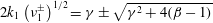 $2k_{1}\left(\unicode[STIX]{x1D708}_{1}^{\pm }\right)^{1/2}=\unicode[STIX]{x1D6FE}\pm \sqrt{\unicode[STIX]{x1D6FE}^{2}+4(\unicode[STIX]{x1D6FD}-1)}$
for parameters such that the right-hand side is real and positive. Then, if
$2k_{1}\left(\unicode[STIX]{x1D708}_{1}^{\pm }\right)^{1/2}=\unicode[STIX]{x1D6FE}\pm \sqrt{\unicode[STIX]{x1D6FE}^{2}+4(\unicode[STIX]{x1D6FD}-1)}$
for parameters such that the right-hand side is real and positive. Then, if
 $\unicode[STIX]{x1D6FE}^{2}+4(\unicode[STIX]{x1D6FD}-1)\leqslant 0$
, these purely streamwise modes are always linearly or neutrally stable. If
$\unicode[STIX]{x1D6FE}^{2}+4(\unicode[STIX]{x1D6FD}-1)\leqslant 0$
, these purely streamwise modes are always linearly or neutrally stable. If
 $\unicode[STIX]{x1D6FD}>1$
, there is linear instability for the
$\unicode[STIX]{x1D6FD}>1$
, there is linear instability for the
 $(k_{1},0)$
-mode in the region
$(k_{1},0)$
-mode in the region
 $\unicode[STIX]{x1D708}_{1}<\unicode[STIX]{x1D708}_{1}^{+}$
, and if
$\unicode[STIX]{x1D708}_{1}<\unicode[STIX]{x1D708}_{1}^{+}$
, and if
 $\unicode[STIX]{x1D6FD}\leqslant 1$
and
$\unicode[STIX]{x1D6FD}\leqslant 1$
and
 $\unicode[STIX]{x1D6FE}^{2}\,+\,4(\unicode[STIX]{x1D6FD}\,-\,1)\,>\,0$
, there is a band of instability in the interval
$\unicode[STIX]{x1D6FE}^{2}\,+\,4(\unicode[STIX]{x1D6FD}\,-\,1)\,>\,0$
, there is a band of instability in the interval
 $\unicode[STIX]{x1D708}_{1}^{-}<\unicode[STIX]{x1D708}_{1}<\unicode[STIX]{x1D708}_{1}^{+}$
, where
$\unicode[STIX]{x1D708}_{1}^{-}<\unicode[STIX]{x1D708}_{1}<\unicode[STIX]{x1D708}_{1}^{+}$
, where
 $\unicode[STIX]{x1D708}_{1}^{\pm }$
are
$\unicode[STIX]{x1D708}_{1}^{\pm }$
are
 $$\begin{eqnarray}\unicode[STIX]{x1D708}_{1}^{\pm }=\frac{\unicode[STIX]{x1D6FE}^{2}+2(\unicode[STIX]{x1D6FD}-1)\pm \unicode[STIX]{x1D6FE}\sqrt{\unicode[STIX]{x1D6FE}^{2}+4(\unicode[STIX]{x1D6FD}-1)}}{2k_{1}^{2}}.\end{eqnarray}$$
Similarly for the purely transverse
 $(0,k_{2})$
-mode, equation (4.14) gives the straight line neutral curves defined by
$(0,k_{2})$
-mode, equation (4.14) gives the straight line neutral curves defined by
 $2k_{2}\left(\unicode[STIX]{x1D708}_{2}^{\pm }\right)^{1/2}=\unicode[STIX]{x1D6FE}\pm \sqrt{\unicode[STIX]{x1D6FE}^{2}-4}$
, and it follows that we have linear or neutral stability for
$2k_{2}\left(\unicode[STIX]{x1D708}_{2}^{\pm }\right)^{1/2}=\unicode[STIX]{x1D6FE}\pm \sqrt{\unicode[STIX]{x1D6FE}^{2}-4}$
, and it follows that we have linear or neutral stability for
 $\unicode[STIX]{x1D6FE}\leqslant 2$
, while for
$\unicode[STIX]{x1D6FE}\leqslant 2$
, while for
 $\unicode[STIX]{x1D6FE}>2$
there is a strip of linear instability in the
$\unicode[STIX]{x1D6FE}>2$
there is a strip of linear instability in the
 $\unicode[STIX]{x1D708}_{2}-$
interval
$\unicode[STIX]{x1D708}_{2}-$
interval
 $$\begin{eqnarray}\frac{\unicode[STIX]{x1D6FE}^{2}-2-\unicode[STIX]{x1D6FE}\sqrt{\unicode[STIX]{x1D6FE}^{2}-4}}{2k_{2}^{2}}<\unicode[STIX]{x1D708}_{2}<\frac{\unicode[STIX]{x1D6FE}^{2}-2+\unicode[STIX]{x1D6FE}\sqrt{\unicode[STIX]{x1D6FE}^{2}-4}}{2k_{2}^{2}}.\end{eqnarray}$$
Hence
 $\unicode[STIX]{x1D6FE}\leqslant 2$
is precisely the condition we need to impose in order to study (4.7) for any domain dimensions; this ensures that the
$\unicode[STIX]{x1D6FE}\leqslant 2$
is precisely the condition we need to impose in order to study (4.7) for any domain dimensions; this ensures that the
 $y$
-modes are always damped, except for
$y$
-modes are always damped, except for
 $\unicode[STIX]{x1D6FE}=2$
, when these modes can be neutrally stable at distinct values of
$\unicode[STIX]{x1D6FE}=2$
, when these modes can be neutrally stable at distinct values of
 $L_{2}$
. This restriction on
$L_{2}$
. This restriction on
 $\unicode[STIX]{x1D6FE}$
translates back to the requirement that
$\unicode[STIX]{x1D6FE}$
translates back to the requirement that
 $$\begin{eqnarray}We\leqslant \left(\frac{2\cot \unicode[STIX]{x1D703}}{C}\right)^{1/2}.\end{eqnarray}$$
Figure 2. Linear stability regions for
 $\unicode[STIX]{x1D6FE}=2$
and a range of Reynolds numbers. The number of unstable modes within regions in the
$\unicode[STIX]{x1D6FE}=2$
and a range of Reynolds numbers. The number of unstable modes within regions in the
 $\unicode[STIX]{x1D708}_{1}$
–
$\unicode[STIX]{x1D708}_{1}$
–
 $\unicode[STIX]{x1D708}_{2}$
plane is displayed, where we have only counted the pairs or quartets of modes as one. The diagonal lines correspond to
$\unicode[STIX]{x1D708}_{2}$
plane is displayed, where we have only counted the pairs or quartets of modes as one. The diagonal lines correspond to
 $\unicode[STIX]{x1D708}_{1}=\unicode[STIX]{x1D708}_{2}$
along which we perform numerical simulations.
$\unicode[STIX]{x1D708}_{1}=\unicode[STIX]{x1D708}_{2}$
along which we perform numerical simulations.
This condition does not imply that the mixed Fourier modes are also linearly stable. Finding the neutral stability curves can be done analytically, but the determination of the number of unstable modes in each instability region is best done numerically in a straightforward manner; for particular values of the parameters
 $\unicode[STIX]{x1D6FD}$
and
$\unicode[STIX]{x1D6FD}$
and
 $\unicode[STIX]{x1D6FE}$
, the regions of stability in the
$\unicode[STIX]{x1D6FE}$
, the regions of stability in the
 $\unicode[STIX]{x1D708}_{1}$
–
$\unicode[STIX]{x1D708}_{1}$
–
 $\unicode[STIX]{x1D708}_{2}$
plane are quite complicated. Recall that
$\unicode[STIX]{x1D708}_{2}$
plane are quite complicated. Recall that
 $\unicode[STIX]{x1D6FD}=1$
corresponds to taking the critical Reynolds number for the flow,
$\unicode[STIX]{x1D6FD}=1$
corresponds to taking the critical Reynolds number for the flow,
 $Re_{c}=5\cot \unicode[STIX]{x1D703}/4$
, with
$Re_{c}=5\cot \unicode[STIX]{x1D703}/4$
, with
 $\unicode[STIX]{x1D6FD}<1$
(
$\unicode[STIX]{x1D6FD}<1$
(
 $\unicode[STIX]{x1D6FD}>1$
) being subcritical (supercritical). For the subcritical case, we will show numerical simulations for
$\unicode[STIX]{x1D6FD}>1$
) being subcritical (supercritical). For the subcritical case, we will show numerical simulations for
 $\unicode[STIX]{x1D6FD}=0.01$
and
$\unicode[STIX]{x1D6FD}=0.01$
and
 $\unicode[STIX]{x1D6FD}=0.5$
, and for the supercritical case we compute with
$\unicode[STIX]{x1D6FD}=0.5$
, and for the supercritical case we compute with
 $\unicode[STIX]{x1D6FD}=2$
. The linear stability regions for these values of
$\unicode[STIX]{x1D6FD}=2$
. The linear stability regions for these values of
 $\unicode[STIX]{x1D6FD}$
, along with the critical case
$\unicode[STIX]{x1D6FD}$
, along with the critical case
 $\unicode[STIX]{x1D6FD}=1$
, are shown in figure 2 with the maximum allowable electric field strength
$\unicode[STIX]{x1D6FD}=1$
, are shown in figure 2 with the maximum allowable electric field strength
 $\unicode[STIX]{x1D6FE}=2$
. This value of
$\unicode[STIX]{x1D6FE}=2$
. This value of
 $\unicode[STIX]{x1D6FE}$
gives unstable wavenumbers for all values of
$\unicode[STIX]{x1D6FE}$
gives unstable wavenumbers for all values of
 $\unicode[STIX]{x1D6FD}>0$
, hence the dynamics for small subcritical Reynolds numbers is non-trivial on sufficiently large domains. Figure 2(a) has a relatively small value with
$\unicode[STIX]{x1D6FD}>0$
, hence the dynamics for small subcritical Reynolds numbers is non-trivial on sufficiently large domains. Figure 2(a) has a relatively small value with
 $\unicode[STIX]{x1D6FD}=0.01$
, and shows distinct behaviour from the other cases in panels (b–d); there are regions of linear stability (no unstable modes depicted with white) in-between regions of linear instability. A subcritical Reynolds number, corresponding to
$\unicode[STIX]{x1D6FD}=0.01$
, and shows distinct behaviour from the other cases in panels (b–d); there are regions of linear stability (no unstable modes depicted with white) in-between regions of linear instability. A subcritical Reynolds number, corresponding to
 $\unicode[STIX]{x1D6FD}<1$
, is a necessary condition for the existence of such stable regions, but is not sufficient, as can be seen from the results in figure 2(b) for
$\unicode[STIX]{x1D6FD}<1$
, is a necessary condition for the existence of such stable regions, but is not sufficient, as can be seen from the results in figure 2(b) for
 $\unicode[STIX]{x1D6FD}=0.5$
. As expected, the number of unstable modes increases as
$\unicode[STIX]{x1D6FD}=0.5$
. As expected, the number of unstable modes increases as
 $\unicode[STIX]{x1D708}_{1}$
and
$\unicode[STIX]{x1D708}_{1}$
and
 $\unicode[STIX]{x1D708}_{2}$
decrease (analogous to the domain size increasing). Note also that in the figure, due to the symmetries of the dispersion relation (4.14), we count the quartet of unstable modes
$\unicode[STIX]{x1D708}_{2}$
decrease (analogous to the domain size increasing). Note also that in the figure, due to the symmetries of the dispersion relation (4.14), we count the quartet of unstable modes
 $(k_{1},k_{2})$
,
$(k_{1},k_{2})$
,
 $(k_{1},-k_{2})$
,
$(k_{1},-k_{2})$
,
 $(-k_{1},k_{2})$
,
$(-k_{1},k_{2})$
,
 $(-k_{1},-k_{2})$
as one, with obvious special cases when either
$(-k_{1},-k_{2})$
as one, with obvious special cases when either
 $k_{1}$
or
$k_{1}$
or
 $k_{2}$
are zero. Regions in parameter space where there are no unstable modes give solutions of (4.7) that decay to the trivial zero solution, as can be shown analytically. An energy equation giving the evolution of the
$k_{2}$
are zero. Regions in parameter space where there are no unstable modes give solutions of (4.7) that decay to the trivial zero solution, as can be shown analytically. An energy equation giving the evolution of the
 $L^{2}$
-norm of
$L^{2}$
-norm of
 $\unicode[STIX]{x1D702}$
may be constructed by multiplying (4.7) by
$\unicode[STIX]{x1D702}$
may be constructed by multiplying (4.7) by
 $\unicode[STIX]{x1D702}$
, and integrating over
$\unicode[STIX]{x1D702}$
, and integrating over
 $Q$
. The resulting equation has no contribution from the nonlinear term due to the periodic boundary conditions. From this, it may be observed that if
$Q$
. The resulting equation has no contribution from the nonlinear term due to the periodic boundary conditions. From this, it may be observed that if
 $s(\tilde{\boldsymbol{k}})<0$
for all non-zero
$s(\tilde{\boldsymbol{k}})<0$
for all non-zero
 $\boldsymbol{k}\in \mathbb{Z}^{2}$
, an exponentially decaying bound on the
$\boldsymbol{k}\in \mathbb{Z}^{2}$
, an exponentially decaying bound on the
 $L^{2}$
-norm of
$L^{2}$
-norm of
 $\unicode[STIX]{x1D702}$
is obtained. Maximum exponential growth rates may be obtained in a similar way. For subcritical Reynolds number flows,
$\unicode[STIX]{x1D702}$
is obtained. Maximum exponential growth rates may be obtained in a similar way. For subcritical Reynolds number flows,
 $\unicode[STIX]{x1D6FD}<1$
, with the condition that the electric field strength is sufficiently weak,
$\unicode[STIX]{x1D6FD}<1$
, with the condition that the electric field strength is sufficiently weak,
 $\unicode[STIX]{x1D6FE}<2(1-\unicode[STIX]{x1D6FD})^{1/2}$
, all Fourier modes are linearly stable for any choice of length parameters, and hence all solutions decay to zero. The case of
$\unicode[STIX]{x1D6FE}<2(1-\unicode[STIX]{x1D6FD})^{1/2}$
, all Fourier modes are linearly stable for any choice of length parameters, and hence all solutions decay to zero. The case of
 $\unicode[STIX]{x1D6FE}=2(1-\unicode[STIX]{x1D6FD})^{1/2}$
for a subcritical flow corresponds to the critical electric field strength identified by González & Castellanos (Reference González and Castellanos1996) for the one-dimensional equation (1.1) (where the
$\unicode[STIX]{x1D6FE}=2(1-\unicode[STIX]{x1D6FD})^{1/2}$
for a subcritical flow corresponds to the critical electric field strength identified by González & Castellanos (Reference González and Castellanos1996) for the one-dimensional equation (1.1) (where the
 $-$
is taken), above which the flat film solution becomes unstable for sufficiently large domain lengths. For other choices of
$-$
is taken), above which the flat film solution becomes unstable for sufficiently large domain lengths. For other choices of
 $\unicode[STIX]{x1D6FD}$
and
$\unicode[STIX]{x1D6FD}$
and
 $\unicode[STIX]{x1D6FE}$
, unstable wavenumbers may not be attained by the discrete spectrum, thus there will be a condition on
$\unicode[STIX]{x1D6FE}$
, unstable wavenumbers may not be attained by the discrete spectrum, thus there will be a condition on
 $L_{1}$
and
$L_{1}$
and
 $L_{2}$
to determine whether the solution decays to zero – this was discussed for the one-dimensional equation by Tseluiko & Papageorgiou (Reference Tseluiko and Papageorgiou2006b
), however it is more complicated for our two-dimensional problem and does not add to our exposition. Nevertheless, for
$L_{2}$
to determine whether the solution decays to zero – this was discussed for the one-dimensional equation by Tseluiko & Papageorgiou (Reference Tseluiko and Papageorgiou2006b
), however it is more complicated for our two-dimensional problem and does not add to our exposition. Nevertheless, for
 $\unicode[STIX]{x1D6FD}\leqslant 1$
and
$\unicode[STIX]{x1D6FD}\leqslant 1$
and
 $\unicode[STIX]{x1D6FE}>2(1-\unicode[STIX]{x1D6FD})^{1/2}$
, or for
$\unicode[STIX]{x1D6FE}>2(1-\unicode[STIX]{x1D6FD})^{1/2}$
, or for
 $\unicode[STIX]{x1D6FD}>1$
, the first bifurcation can be shown to always occur at
$\unicode[STIX]{x1D6FD}>1$
, the first bifurcation can be shown to always occur at
 $$\begin{eqnarray}L_{1}=\frac{4\unicode[STIX]{x03C0}}{\unicode[STIX]{x1D6FE}+\sqrt{\unicode[STIX]{x1D6FE}^{2}+4(\unicode[STIX]{x1D6FD}-1)}}\end{eqnarray}$$
when the
 $(1,0)$
-mode first becomes linearly unstable. However, the flow may stabilise again as observed in figure 2(a).
$(1,0)$
-mode first becomes linearly unstable. However, the flow may stabilise again as observed in figure 2(a).
4.3 Numerical method
We now move on to a numerical study of (4.7) on
 $Q$
-periodic domains for which we use the Fourier series representation of the solution,
$Q$
-periodic domains for which we use the Fourier series representation of the solution,
 $$\begin{eqnarray}\unicode[STIX]{x1D702}(\boldsymbol{x},t)=\mathop{\sum }_{\boldsymbol{k}\in \mathbb{Z}^{2}}\unicode[STIX]{x1D702}_{\boldsymbol{k}}(t)\text{e}^{\text{i}\tilde{\boldsymbol{k}}\boldsymbol{\cdot }\boldsymbol{x}},\end{eqnarray}$$
where
 $\unicode[STIX]{x1D702}_{-\boldsymbol{k}}$
is the complex conjugate of
$\unicode[STIX]{x1D702}_{-\boldsymbol{k}}$
is the complex conjugate of
 $\unicode[STIX]{x1D702}_{\boldsymbol{k}}$
since
$\unicode[STIX]{x1D702}_{\boldsymbol{k}}$
since
 $\unicode[STIX]{x1D702}$
is real-valued. We denote the norm and inner product on the space
$\unicode[STIX]{x1D702}$
is real-valued. We denote the norm and inner product on the space
 $L^{2}=L_{per}^{2}(Q)$
as
$L^{2}=L_{per}^{2}(Q)$
as
 $$\begin{eqnarray}|\unicode[STIX]{x1D702}|_{2}=\left(\int _{Q}\unicode[STIX]{x1D702}^{2}\,\text{d}\boldsymbol{x}\right)^{1/2}=|Q|^{1/2}\left(\mathop{\sum }_{\boldsymbol{k}\in \mathbb{Z}^{2}}|\unicode[STIX]{x1D702}_{\boldsymbol{k}}|^{2}\right)^{1/2},\quad \langle \unicode[STIX]{x1D702},u\rangle _{2}=\int _{Q}\unicode[STIX]{x1D702}u\,\text{d}\boldsymbol{x}=|Q|\mathop{\sum }_{\boldsymbol{k}\in \mathbb{Z}^{2}}\unicode[STIX]{x1D702}_{\boldsymbol{k}}u_{-\boldsymbol{k}},\end{eqnarray}$$
respectively, where
 $|Q|=L_{1}L_{2}$
. We utilise a second-order implicit–explicit backwards differentiation formula (BDF) method which belongs to a family of numerical schemes constructed by Akrivis & Crouzeix (Reference Akrivis and Crouzeix2004) for a class of nonlinear parabolic equations under appropriate assumptions on the linear and nonlinear terms. They considered evolution equations of the form
$|Q|=L_{1}L_{2}$
. We utilise a second-order implicit–explicit backwards differentiation formula (BDF) method which belongs to a family of numerical schemes constructed by Akrivis & Crouzeix (Reference Akrivis and Crouzeix2004) for a class of nonlinear parabolic equations under appropriate assumptions on the linear and nonlinear terms. They considered evolution equations of the form
 $$\begin{eqnarray}\unicode[STIX]{x1D702}_{t}+{\mathcal{A}}\unicode[STIX]{x1D702}={\mathcal{B}}(\unicode[STIX]{x1D702}),\end{eqnarray}$$
where
 ${\mathcal{A}}$
is a positive definite, self-adjoint linear operator, and
${\mathcal{A}}$
is a positive definite, self-adjoint linear operator, and
 ${\mathcal{B}}$
is a nonlinear operator which satisfies a local Lipschitz condition. It was shown that these numerical schemes are efficient, convergent and unconditionally stable. For our consideration of (4.7), we have
${\mathcal{B}}$
is a nonlinear operator which satisfies a local Lipschitz condition. It was shown that these numerical schemes are efficient, convergent and unconditionally stable. For our consideration of (4.7), we have
 $$\begin{eqnarray}{\mathcal{A}}\unicode[STIX]{x1D702}=(\unicode[STIX]{x1D6FD}-1)\unicode[STIX]{x1D702}_{xx}-\unicode[STIX]{x1D702}_{yy}+\unicode[STIX]{x1D6FE}\unicode[STIX]{x0394}{\mathcal{R}}(\unicode[STIX]{x1D702})+\unicode[STIX]{x1D6E5}^{2}\unicode[STIX]{x1D702}+c\unicode[STIX]{x1D702},\quad {\mathcal{B}}(\unicode[STIX]{x1D702})=-\unicode[STIX]{x1D702}\unicode[STIX]{x1D702}_{x}+c\unicode[STIX]{x1D702},\end{eqnarray}$$
where the constant
 $c$
is chosen to ensure that
$c$
is chosen to ensure that
 ${\mathcal{A}}$
is positive definite (see appendix A). It follows simply that the linear operator
${\mathcal{A}}$
is positive definite (see appendix A). It follows simply that the linear operator
 ${\mathcal{R}}$
is self-adjoint in
${\mathcal{R}}$
is self-adjoint in
 $L^{2}$
, and thus
$L^{2}$
, and thus
 ${\mathcal{A}}$
is also a self-adjoint linear operator. The local Lipschitz condition for the nonlinear operator
${\mathcal{A}}$
is also a self-adjoint linear operator. The local Lipschitz condition for the nonlinear operator
 ${\mathcal{B}}$
is proved by Akrivis et al. (Reference Akrivis, Kalogirou, Papageorgiou and Smyrlis2016) and therefore the linearly implicit methods derived by Akrivis & Crouzeix (Reference Akrivis and Crouzeix2004) are good candidates and are used for our problem.
${\mathcal{B}}$
is proved by Akrivis et al. (Reference Akrivis, Kalogirou, Papageorgiou and Smyrlis2016) and therefore the linearly implicit methods derived by Akrivis & Crouzeix (Reference Akrivis and Crouzeix2004) are good candidates and are used for our problem.
Let
 $H^{n}$
be the approximation of the solution
$H^{n}$
be the approximation of the solution
 $\unicode[STIX]{x1D702}$
at time
$\unicode[STIX]{x1D702}$
at time
 $n\unicode[STIX]{x0394}t$
for time step
$n\unicode[STIX]{x0394}t$
for time step
 $\unicode[STIX]{x0394}t$
and
$\unicode[STIX]{x0394}t$
and
 $n\in \mathbb{N}$
obtained by splitting the spatial domain
$n\in \mathbb{N}$
obtained by splitting the spatial domain
 $Q$
into
$Q$
into
 $M\times N$
equidistant points, and let
$M\times N$
equidistant points, and let
 $\tilde{{\mathcal{A}}}$
and
$\tilde{{\mathcal{A}}}$
and
 $\tilde{{\mathcal{B}}}$
be the discretisations of
$\tilde{{\mathcal{B}}}$
be the discretisations of
 ${\mathcal{A}}$
and
${\mathcal{A}}$
and
 ${\mathcal{B}}$
, respectively. Taking
${\mathcal{B}}$
, respectively. Taking
 $H^{0}$
as the discretisation of the initial condition
$H^{0}$
as the discretisation of the initial condition
 $\unicode[STIX]{x1D702}_{0}$
, we employ one step of the implicit Euler method as a starting approximation,
$\unicode[STIX]{x1D702}_{0}$
, we employ one step of the implicit Euler method as a starting approximation,
 $$\begin{eqnarray}H^{1}+\unicode[STIX]{x0394}t\tilde{{\mathcal{A}}}H^{1}=H^{0}+\unicode[STIX]{x0394}t\tilde{{\mathcal{B}}}(H^{0}),\end{eqnarray}$$
and then use the second-order implicit–explicit BDF scheme
 $$\begin{eqnarray}\frac{3}{2}H^{n+2}+\unicode[STIX]{x0394}t\tilde{{\mathcal{A}}}H^{n+2}=2H^{n+1}-\frac{1}{2}H^{n}+2\unicode[STIX]{x0394}t\tilde{{\mathcal{B}}}(H^{n+1})-\unicode[STIX]{x0394}t\tilde{{\mathcal{B}}}(H^{n}).\end{eqnarray}$$
We take the discrete Fourier transform of these equations, denoted by
 ${\mathcal{F}}$
, and solve the resulting equations in Fourier space. Let
${\mathcal{F}}$
, and solve the resulting equations in Fourier space. Let
 $\widehat{{\mathcal{A}}}$
be the discretisation of the operator
$\widehat{{\mathcal{A}}}$
be the discretisation of the operator
 ${\mathcal{A}}$
in Fourier space, it is a matrix operator with
${\mathcal{A}}$
in Fourier space, it is a matrix operator with
 $$\begin{eqnarray}\widehat{{\mathcal{A}}}_{\boldsymbol{k}}=-(\unicode[STIX]{x1D6FD}-1)\tilde{k}_{1}^{2}+\tilde{k}_{2}^{2}-\unicode[STIX]{x1D6FE}(\tilde{k}_{1}^{2}+\tilde{k}_{2}^{2})^{3/2}+(\tilde{k}_{1}^{2}+\tilde{k}_{2}^{2})^{2}+c,\end{eqnarray}$$
so that
 $$\begin{eqnarray}{\mathcal{F}}(\tilde{{\mathcal{A}}}(H^{n}))_{\boldsymbol{ k}}=\widehat{{\mathcal{A}}}_{\boldsymbol{k}}\widehat{H}_{\boldsymbol{k}}^{n},\end{eqnarray}$$
where
 $\widehat{H}^{n}$
is the discrete Fourier transform of
$\widehat{H}^{n}$
is the discrete Fourier transform of
 $H^{n}$
. The discrete Fourier transform of the nonlinear operator
$H^{n}$
. The discrete Fourier transform of the nonlinear operator
 ${\mathcal{B}}$
is given by
${\mathcal{B}}$
is given by
 $$\begin{eqnarray}{\mathcal{F}}(\tilde{{\mathcal{B}}}(H^{n}))_{\boldsymbol{ k}}=-\frac{\text{i}\tilde{k}_{1}}{2}{\mathcal{F}}((H^{n})^{2})_{\boldsymbol{ k}}+c\widehat{H}_{\boldsymbol{k}}^{n}.\end{eqnarray}$$
Taking the discrete Fourier transform of (4.23) and (4.24), for the implicit Euler step we obtain
 $$\begin{eqnarray}\widehat{H}_{\boldsymbol{k}}^{1}=\frac{\widehat{H}_{\boldsymbol{k}}^{0}+\unicode[STIX]{x0394}t{\mathcal{F}}(\tilde{{\mathcal{B}}}(H^{0}))_{\boldsymbol{ k}}}{1+\unicode[STIX]{x0394}t\widehat{{\mathcal{A}}}_{\boldsymbol{k}}},\end{eqnarray}$$
and for the second-order BDF steps
 $$\begin{eqnarray}\widehat{H}_{\boldsymbol{k}}^{n+2}=\frac{4\widehat{H}_{\boldsymbol{k}}^{n+1}-\widehat{H}_{\boldsymbol{ k}}^{n}+4\unicode[STIX]{x0394}t{\mathcal{F}}(\tilde{{\mathcal{B}}}(H^{n+1}))_{\boldsymbol{ k}}-2\unicode[STIX]{x0394}t{\mathcal{F}}(\tilde{{\mathcal{B}}}(H^{n}))_{\boldsymbol{ k}}}{3+2\unicode[STIX]{x0394}t\widehat{{\mathcal{A}}}_{\boldsymbol{k}}}.\end{eqnarray}$$
The initial conditions with zero spatial average used in our numerical simulations are
 $$\begin{eqnarray}\unicode[STIX]{x1D702}_{0}(\boldsymbol{x})=\mathop{\sum }_{|\boldsymbol{k}|_{\infty }=1}^{20}a_{\boldsymbol{ k}}\cos (\tilde{\boldsymbol{k}}\boldsymbol{\cdot }\boldsymbol{x})+b_{\boldsymbol{k}}\sin (\tilde{\boldsymbol{k}}\boldsymbol{\cdot }\boldsymbol{x}),\end{eqnarray}$$
where the coefficients
 $a_{\boldsymbol{k}}$
and
$a_{\boldsymbol{k}}$
and
 $b_{\boldsymbol{k}}$
are random numbers from the interval
$b_{\boldsymbol{k}}$
are random numbers from the interval
 $(-0.05,0.05)$
.
$(-0.05,0.05)$
.
4.4 Numerical results
We do not carry out an exhaustive computational study of the dynamics as the lengths
 $L_{1}$
and
$L_{1}$
and
 $L_{2}$
vary independently, due to the large number of runs required producing a significant amount of data to be analysed. Instead, we restrict our attention to square periodic domains by setting
$L_{2}$
vary independently, due to the large number of runs required producing a significant amount of data to be analysed. Instead, we restrict our attention to square periodic domains by setting
 $L_{1}=L_{2}=L$
, or equivalently
$L_{1}=L_{2}=L$
, or equivalently
 $\unicode[STIX]{x1D708}_{1}=\unicode[STIX]{x1D708}_{2}=\unicode[STIX]{x1D708}$
. For subcritical Reynolds numbers we take
$\unicode[STIX]{x1D708}_{1}=\unicode[STIX]{x1D708}_{2}=\unicode[STIX]{x1D708}$
. For subcritical Reynolds numbers we take
 $\unicode[STIX]{x1D6FD}=0.01$
and
$\unicode[STIX]{x1D6FD}=0.01$
and
 $\unicode[STIX]{x1D6FD}=0.5$
, and as noted previously, these have very different linear stability regions as seen in figure 2(a,b). For supercritical Reynolds numbers (the dynamics is non-trivial even in the absence of a field with
$\unicode[STIX]{x1D6FD}=0.5$
, and as noted previously, these have very different linear stability regions as seen in figure 2(a,b). For supercritical Reynolds numbers (the dynamics is non-trivial even in the absence of a field with
 $\unicode[STIX]{x1D6FE}=0$
) we take
$\unicode[STIX]{x1D6FE}=0$
) we take
 $\unicode[STIX]{x1D6FD}=2$
, and provide a qualitative description of the dynamics as
$\unicode[STIX]{x1D6FD}=2$
, and provide a qualitative description of the dynamics as
 $\unicode[STIX]{x1D6FE}$
is increased. We will examine the attractor windows of dynamical behaviours in the bifurcation parameter
$\unicode[STIX]{x1D6FE}$
is increased. We will examine the attractor windows of dynamical behaviours in the bifurcation parameter
 $L$
(and
$L$
(and
 $\unicode[STIX]{x1D708}$
also), in particular obtaining wave formations which are not dominated by one-dimensional behaviour. To provide a qualitative description of solutions to (4.7) and the nature of the attractor, we employ a number of data analysis tools. We use the
$\unicode[STIX]{x1D708}$
also), in particular obtaining wave formations which are not dominated by one-dimensional behaviour. To provide a qualitative description of solutions to (4.7) and the nature of the attractor, we employ a number of data analysis tools. We use the
 $L^{2}$
-norm as a measure of the solution energy, defining
$L^{2}$
-norm as a measure of the solution energy, defining
 $$\begin{eqnarray}E(t)=|\unicode[STIX]{x1D702}(t)|_{2}.\end{eqnarray}$$
From this we construct the phase plane diagram for the energy, plotting
 $E(t)$
against
$E(t)$
against
 ${\dot{E}}(t)$
. To construct the Poincaré energy return map, we find the sequence of times
${\dot{E}}(t)$
. To construct the Poincaré energy return map, we find the sequence of times
 $\{t_{n}\}_{n=1}^{N}$
when
$\{t_{n}\}_{n=1}^{N}$
when
 $E$
is at a minimum over a large time interval. We then plot the points
$E$
is at a minimum over a large time interval. We then plot the points
 $(E_{n},E_{n+1})$
where
$(E_{n},E_{n+1})$
where
 $E_{n}=E(t_{n})$
. The two-dimensionality of solutions to (4.7) is quantified by studying the time-averaged power spectrum of solutions, given by
$E_{n}=E(t_{n})$
. The two-dimensionality of solutions to (4.7) is quantified by studying the time-averaged power spectrum of solutions, given by
 $$\begin{eqnarray}S(\boldsymbol{k})=|Q|\lim _{T\rightarrow \infty }\frac{1}{T}\int _{0}^{T}|\unicode[STIX]{x1D702}_{\boldsymbol{ k}}|^{2}\,\text{d}t\end{eqnarray}$$
for each
 $\boldsymbol{k}\in \mathbb{Z}^{2}$
. In practice, we approximate
$\boldsymbol{k}\in \mathbb{Z}^{2}$
. In practice, we approximate
 $S(\boldsymbol{k})$
by
$S(\boldsymbol{k})$
by
 $$\begin{eqnarray}\overline{S}(\boldsymbol{k})=\frac{|Q|}{T_{2}-T_{1}}\int _{T_{1}}^{T_{2}}|\unicode[STIX]{x1D702}_{\boldsymbol{k}}|^{2}\,\text{d}t,\end{eqnarray}$$
where
 $0\ll T_{1}\ll T_{2}$
are two large times. Any activity in the mixed Fourier modes for solutions in the attractor will be made apparent with this diagnostic; if the time-averaged power spectrum is restricted to the
$0\ll T_{1}\ll T_{2}$
are two large times. Any activity in the mixed Fourier modes for solutions in the attractor will be made apparent with this diagnostic; if the time-averaged power spectrum is restricted to the
 $(k_{1},0)$
-modes, then we will call it one-dimensional, otherwise it is called two-dimensional. The integration times used were at least
$(k_{1},0)$
-modes, then we will call it one-dimensional, otherwise it is called two-dimensional. The integration times used were at least
 $10^{3}$
time units, and Fourier modes of magnitude as small as
$10^{3}$
time units, and Fourier modes of magnitude as small as
 $10^{-15}$
were retained. The time steps used for numerical simulations were
$10^{-15}$
were retained. The time steps used for numerical simulations were
 $10^{-4}$
or smaller; for larger values of
$10^{-4}$
or smaller; for larger values of
 $\unicode[STIX]{x1D6FD}$
and
$\unicode[STIX]{x1D6FD}$
and
 $\unicode[STIX]{x1D6FE}$
, smaller time steps are required to obtain good convergence (for a convergence analysis of the same scheme applied to the Kuramoto–Sivashinsky equation (1.4), see Akrivis et al.
Reference Akrivis, Kalogirou, Papageorgiou and Smyrlis2016). It is worthwhile to question whether there are any issues associated with performing numerical simulations at the critical electric field strength
$\unicode[STIX]{x1D6FE}$
, smaller time steps are required to obtain good convergence (for a convergence analysis of the same scheme applied to the Kuramoto–Sivashinsky equation (1.4), see Akrivis et al.
Reference Akrivis, Kalogirou, Papageorgiou and Smyrlis2016). It is worthwhile to question whether there are any issues associated with performing numerical simulations at the critical electric field strength
 $\unicode[STIX]{x1D6FE}=2$
. From the form of the nonlinearity in (4.7), the problem for the transverse modes (
$\unicode[STIX]{x1D6FE}=2$
. From the form of the nonlinearity in (4.7), the problem for the transverse modes (
 $y$
-modes) is linear and decouples. For
$y$
-modes) is linear and decouples. For
 $\unicode[STIX]{x1D6FE}=2$
, there exist discrete values of
$\unicode[STIX]{x1D6FE}=2$
, there exist discrete values of
 $L_{2}$
at which the transverse modes are neutrally stable, otherwise they are always damped, and so the dynamical behaviour we observe at the endpoint
$L_{2}$
at which the transverse modes are neutrally stable, otherwise they are always damped, and so the dynamical behaviour we observe at the endpoint
 $\unicode[STIX]{x1D6FE}=2$
is not a special case, but can be found for
$\unicode[STIX]{x1D6FE}=2$
is not a special case, but can be found for
 $\unicode[STIX]{x1D6FE}$
slightly less than
$\unicode[STIX]{x1D6FE}$
slightly less than
 $2$
. We note that numerical simulations were also performed for
$2$
. We note that numerical simulations were also performed for
 $\unicode[STIX]{x1D6FE}>2$
, and as predicted by the linear theory, blow-ups are observed for some domain dimensions; this is not surprising given that the transverse mode problem decouples as discussed above.
$\unicode[STIX]{x1D6FE}>2$
, and as predicted by the linear theory, blow-ups are observed for some domain dimensions; this is not surprising given that the transverse mode problem decouples as discussed above.
In our presentation of results, we use the following key for the attractor behaviour:
-
(i)
 $Z$
denotes an attractor consisting of the trivial zero solution.
$Z$
denotes an attractor consisting of the trivial zero solution. -
(ii)
$D_{(k_{1},k_{2})}$
denotes a modal attractor (steady or travelling) in which solutions are dominated by the
$(k_{1}m,\pm k_{2}m)$
-modes where
$m\in \mathbb{Z}$
. For example,
$D_{(2,0)}$
is an attractor of bimodal states in the streamwise direction with solutions dominated by the
$(2m,0)$
-modes. -
(iii)
$TP$
denotes a time-periodic attractor (more specific details of these will be given where appropriate in the following discussion). -
(iv)
$A$
denotes a range of attractors with complicated dynamical behaviour, including period-doubling bifurcations, multimodal steady or travelling waves, time-periodic/quasi-periodic attractors, periodic bursting and chaotic attractors.


For the attractors denoted by
 $TP$
or
$TP$
or
 $A$
, a subscript
$A$
, a subscript
 $1$
or
$1$
or
 $2$
indicates whether the attractor dynamics is dominated by one or two-dimensional behaviour, respectively. It is important to note that due to the Galilean transformation (4.1b
) that is used to remove an advective term, all steady states correspond to travelling waves in the original frame of reference.
$2$
indicates whether the attractor dynamics is dominated by one or two-dimensional behaviour, respectively. It is important to note that due to the Galilean transformation (4.1b
) that is used to remove an advective term, all steady states correspond to travelling waves in the original frame of reference.

Figure 3. Schematic of the attractors for
 $\unicode[STIX]{x1D6FD}=0.01$
,
$\unicode[STIX]{x1D6FD}=0.01$
,
 $\unicode[STIX]{x1D6FE}=2$
.
$\unicode[STIX]{x1D6FE}=2$
.
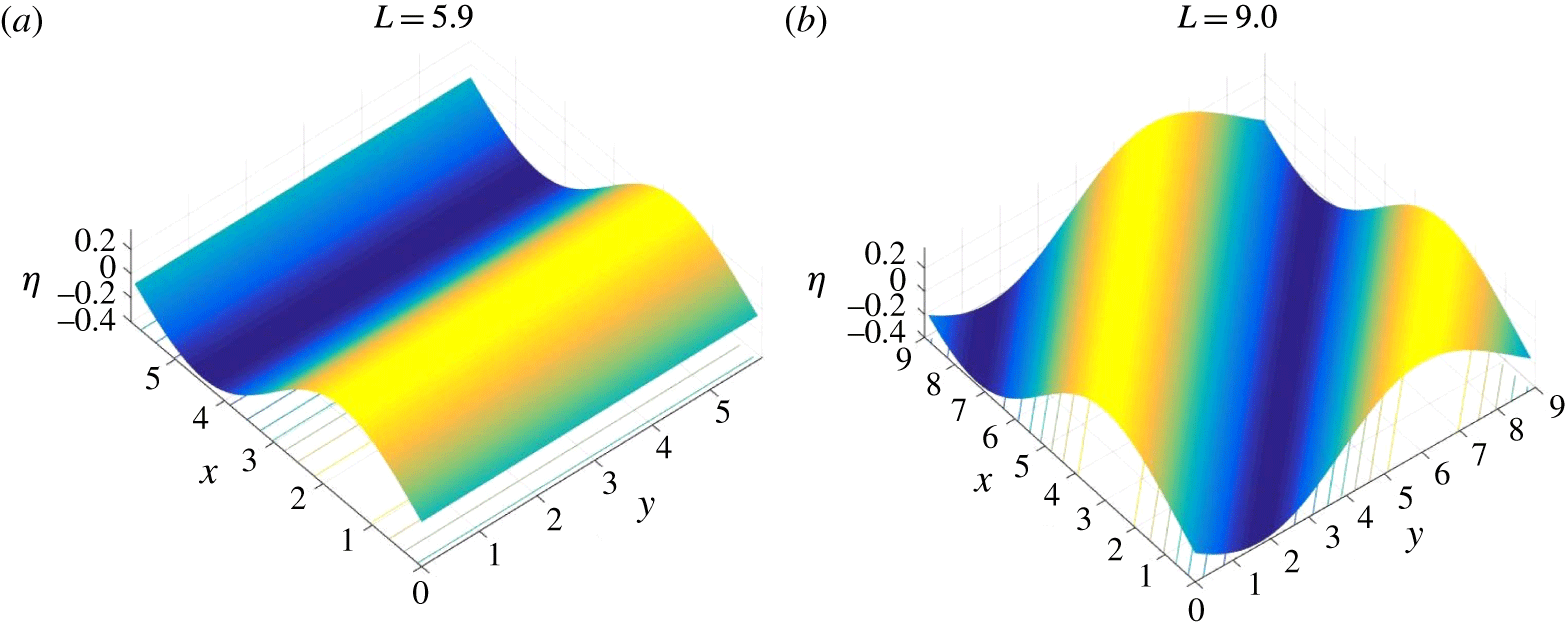
Figure 4. Profiles of solutions in
 $D_{(1,0)}$
and
$D_{(1,0)}$
and
 $D_{(1,1)}$
for
$D_{(1,1)}$
for
 $\unicode[STIX]{x1D6FD}=0.01$
,
$\unicode[STIX]{x1D6FD}=0.01$
,
 $\unicode[STIX]{x1D6FE}=2$
.
$\unicode[STIX]{x1D6FE}=2$
.
4.4.1 Small subcritical Reynolds number,
$\unicode[STIX]{x1D6FD}=0.01$

For
 $\unicode[STIX]{x1D6FD}=0.01$
and
$\unicode[STIX]{x1D6FD}=0.01$
and
 $\unicode[STIX]{x1D6FE}<2\sqrt{0.99}\approx 1.9900$
, we have decay of all solutions to zero for arbitrary initial conditions, and so we concentrate on the case of
$\unicode[STIX]{x1D6FE}<2\sqrt{0.99}\approx 1.9900$
, we have decay of all solutions to zero for arbitrary initial conditions, and so we concentrate on the case of
 $\unicode[STIX]{x1D6FE}=2$
. The linear stability regions for this choice of
$\unicode[STIX]{x1D6FE}=2$
. The linear stability regions for this choice of
 $\unicode[STIX]{x1D6FE}$
are depicted in figure 2(a), and following the line along which the numerical results are obtained (
$\unicode[STIX]{x1D6FE}$
are depicted in figure 2(a), and following the line along which the numerical results are obtained (
 $\unicode[STIX]{x1D708}_{1}=\unicode[STIX]{x1D708}_{2}$
), initially there is alternation between linear stability and instability. Figure 3 was constructed from a large number of numerical experiments to collect a broad, qualitative description of the solution attractors. As
$\unicode[STIX]{x1D708}_{1}=\unicode[STIX]{x1D708}_{2}$
), initially there is alternation between linear stability and instability. Figure 3 was constructed from a large number of numerical experiments to collect a broad, qualitative description of the solution attractors. As
 $L$
increases, the
$L$
increases, the
 $(1,0)$
-mode becomes linearly unstable first at
$(1,0)$
-mode becomes linearly unstable first at
 $L=5.7$
, and an attractor of one-dimensional unimodal steady states and travelling waves is observed (these are analogous to solutions observed for other Kuramoto–Sivashinsky-type equations). An example of such a profile from this unimodal
$L=5.7$
, and an attractor of one-dimensional unimodal steady states and travelling waves is observed (these are analogous to solutions observed for other Kuramoto–Sivashinsky-type equations). An example of such a profile from this unimodal
 $D_{(1,0)}$
window is given in figure 4(a). Increasing
$D_{(1,0)}$
window is given in figure 4(a). Increasing
 $L$
further to 7.0, the
$L$
further to 7.0, the
 $(1,0)$
-mode then becomes stable again and all initial conditions are attracted to the zero solution – see the schematic in figure 3. This process is repeated when the
$(1,0)$
-mode then becomes stable again and all initial conditions are attracted to the zero solution – see the schematic in figure 3. This process is repeated when the
 $(1,1)$
-mode is destabilised at
$(1,1)$
-mode is destabilised at
 $L=8.3$
, and diagonal unimodal steady states and travelling waves are observed, dominated by the
$L=8.3$
, and diagonal unimodal steady states and travelling waves are observed, dominated by the
 $(k,k)$
-modes or
$(k,k)$
-modes or
 $(k,-k)$
-modes depending on the initial condition. Figure 4(b) shows an example of a solution profile in the attractor of type
$(k,-k)$
-modes depending on the initial condition. Figure 4(b) shows an example of a solution profile in the attractor of type
 $D_{(1,1)}$
. As before, a region of linear stability in all Fourier modes is then reached at
$D_{(1,1)}$
. As before, a region of linear stability in all Fourier modes is then reached at
 $L=9.6$
, and this persists until
$L=9.6$
, and this persists until
 $L=11.4$
. Increasing
$L=11.4$
. Increasing
 $L$
further, we find an increasingly complicated sequence of attractors. For
$L$
further, we find an increasingly complicated sequence of attractors. For
 $L$
between 11.4 and 15.4, at most three modes are linearly unstable – the
$L$
between 11.4 and 15.4, at most three modes are linearly unstable – the
 $(2,0)$
,
$(2,0)$
,
 $(1,2)$
and
$(1,2)$
and
 $(2,1)$
-modes. Initially, increasing
$(2,1)$
-modes. Initially, increasing
 $L$
above 11.4, we see time-periodic and quasi-time-periodic attractors with homoclinic bursting behaviour, where the profile switches between an odd pair (under the parity transformation) of bimodal states through a short two-dimensional pulse transition period (see supplementary movie 1 available at https://doi.org/10.1017/jfm.2017.250 for a time-periodic solution). Beyond
$L$
above 11.4, we see time-periodic and quasi-time-periodic attractors with homoclinic bursting behaviour, where the profile switches between an odd pair (under the parity transformation) of bimodal states through a short two-dimensional pulse transition period (see supplementary movie 1 available at https://doi.org/10.1017/jfm.2017.250 for a time-periodic solution). Beyond
 $L=13.6$
, the
$L=13.6$
, the
 $(1,2)$
-mode dominates and we observe a window of the attractor
$(1,2)$
-mode dominates and we observe a window of the attractor
 $D_{(1,2)}$
. For
$D_{(1,2)}$
. For
 $L$
above 14.7, we mostly find attractors of homoclinic bursting behaviours with long burst times – we observed burst times of
$L$
above 14.7, we mostly find attractors of homoclinic bursting behaviours with long burst times – we observed burst times of
 $O(10^{3})$
time units. All modes become linearly stable again at
$O(10^{3})$
time units. All modes become linearly stable again at
 $L=15.4$
, and non-trivial behaviour is not found until
$L=15.4$
, and non-trivial behaviour is not found until
 $L=16.6$
when the
$L=16.6$
when the
 $(2,2)$
-mode becomes unstable and a
$(2,2)$
-mode becomes unstable and a
 $D_{(2,2)}$
solution emerges. For
$D_{(2,2)}$
solution emerges. For
 $L$
above 18.7, the dynamics becomes increasingly complicated (see supplementary movie 2 for a quasi-time-periodic solution exhibiting homoclinic bursting behaviour for
$L$
above 18.7, the dynamics becomes increasingly complicated (see supplementary movie 2 for a quasi-time-periodic solution exhibiting homoclinic bursting behaviour for
 $L=18.85$
, where the interface undergoes transitions between a pulse state and a ‘snaking’ transverse wave). Finally, fully chaotic behaviour is found for sufficiently large
$L=18.85$
, where the interface undergoes transitions between a pulse state and a ‘snaking’ transverse wave). Finally, fully chaotic behaviour is found for sufficiently large
 $L$
.
$L$
.
4.4.2 Moderate subcritical Reynolds number,
$\unicode[STIX]{x1D6FD}=0.5$

Having considered small inertia effects, we now turn to larger values of
 $\unicode[STIX]{x1D6FD}$
, but still in the subcritical regime. We pick
$\unicode[STIX]{x1D6FD}$
, but still in the subcritical regime. We pick
 $\unicode[STIX]{x1D6FD}=0.5$
, in which case we have decay of all initial conditions to the trivial zero solution for
$\unicode[STIX]{x1D6FD}=0.5$
, in which case we have decay of all initial conditions to the trivial zero solution for
 $\unicode[STIX]{x1D6FE}<\sqrt{2}\approx 1.4142$
. Thus, we will investigate the cases
$\unicode[STIX]{x1D6FE}<\sqrt{2}\approx 1.4142$
. Thus, we will investigate the cases
 $\unicode[STIX]{x1D6FE}=1.5$
and 2 – the linear stability regions for
$\unicode[STIX]{x1D6FE}=1.5$
and 2 – the linear stability regions for
 $\unicode[STIX]{x1D6FD}=0.5$
,
$\unicode[STIX]{x1D6FD}=0.5$
,
 $\unicode[STIX]{x1D6FE}=2$
are displayed in figure 2(b). The figure shows clearly that in contrast to the smaller inertia case
$\unicode[STIX]{x1D6FE}=2$
are displayed in figure 2(b). The figure shows clearly that in contrast to the smaller inertia case
 $\unicode[STIX]{x1D6FD}=0.01$
, there are no regions of stability after the first mode becomes linearly unstable, and hence non-trivial dynamics is expected throughout as
$\unicode[STIX]{x1D6FD}=0.01$
, there are no regions of stability after the first mode becomes linearly unstable, and hence non-trivial dynamics is expected throughout as
 $L$
increases (this can also be observed for
$L$
increases (this can also be observed for
 $\unicode[STIX]{x1D6FE}=1.5$
, except at the discrete value of
$\unicode[STIX]{x1D6FE}=1.5$
, except at the discrete value of
 $L_{1}=4\unicode[STIX]{x03C0}$
). This is confirmed by the results of figure 5, which depicts the most attracting states as
$L_{1}=4\unicode[STIX]{x03C0}$
). This is confirmed by the results of figure 5, which depicts the most attracting states as
 $L$
increases for
$L$
increases for
 $\unicode[STIX]{x1D6FE}=1.5$
and 2.
$\unicode[STIX]{x1D6FE}=1.5$
and 2.
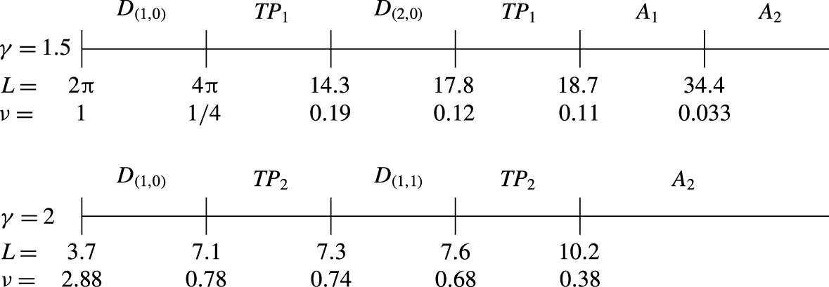
Figure 5. Schematic of the attractors (not drawn to scale) for
 $\unicode[STIX]{x1D6FD}=0.5$
,
$\unicode[STIX]{x1D6FD}=0.5$
,
 $\unicode[STIX]{x1D6FE}=1.5,2$
.
$\unicode[STIX]{x1D6FE}=1.5,2$
.
For
 $\unicode[STIX]{x1D6FE}=1.5$
, the zero solution loses stability to the
$\unicode[STIX]{x1D6FE}=1.5$
, the zero solution loses stability to the
 $(1,0)$
-mode when
$(1,0)$
-mode when
 $L$
exceeds
$L$
exceeds
 $2\unicode[STIX]{x03C0}$
, and a window of unimodal
$2\unicode[STIX]{x03C0}$
, and a window of unimodal
 $D_{(1,0)}$
states emerges. Note that according to linear theory, the
$D_{(1,0)}$
states emerges. Note that according to linear theory, the
 $(1,0)$
-mode becomes stable at
$(1,0)$
-mode becomes stable at
 $L=4\unicode[STIX]{x03C0}$
, and for
$L=4\unicode[STIX]{x03C0}$
, and for
 $L>4\unicode[STIX]{x03C0}$
the
$L>4\unicode[STIX]{x03C0}$
the
 $(2,0)$
-mode loses stability. At
$(2,0)$
-mode loses stability. At
 $L=4\unicode[STIX]{x03C0}$
, we find a Hopf bifurcation with a time-periodic, spatially one-dimensional
$L=4\unicode[STIX]{x03C0}$
, we find a Hopf bifurcation with a time-periodic, spatially one-dimensional
 $TP_{1}$
solution emerging until
$TP_{1}$
solution emerging until
 $L=14.3$
– these solutions are homoclinic bursts with long-lived
$L=14.3$
– these solutions are homoclinic bursts with long-lived
 $D_{(2,0)}$
solutions undergoing time-periodic oscillations through unimodal
$D_{(2,0)}$
solutions undergoing time-periodic oscillations through unimodal
 $D_{(1,0)}$
states (burst times are around 300 time units for values of
$D_{(1,0)}$
states (burst times are around 300 time units for values of
 $L$
away from the boundary of this window). The next attractor window,
$L$
away from the boundary of this window). The next attractor window,
 $14.3<L<17.8$
, contains bimodal
$14.3<L<17.8$
, contains bimodal
 $D_{(2,0)}$
states that in turn lose stability via a Hopf bifurcation to time-periodic solutions (no homoclinic bursting) in the window
$D_{(2,0)}$
states that in turn lose stability via a Hopf bifurcation to time-periodic solutions (no homoclinic bursting) in the window
 $17.8<L<18.7$
. The strong one-dimensionality persists in the window
$17.8<L<18.7$
. The strong one-dimensionality persists in the window
 $18.7<L<34.4$
and complex dynamics including trimodal steady states and chaotic bursting are found. Beyond this, the mixed modes remain active in chaotic solutions, and are characterised by the presence of small deformations on the usual cellular one-dimensional chaotic profiles.
$18.7<L<34.4$
and complex dynamics including trimodal steady states and chaotic bursting are found. Beyond this, the mixed modes remain active in chaotic solutions, and are characterised by the presence of small deformations on the usual cellular one-dimensional chaotic profiles.
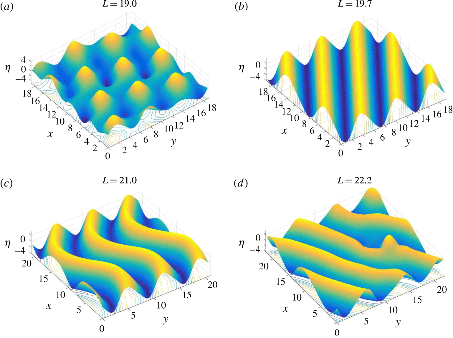
Figure 6. Window
 $A_{2}$
,
$A_{2}$
,
 $\unicode[STIX]{x1D6FD}=0.5$
,
$\unicode[STIX]{x1D6FD}=0.5$
,
 $\unicode[STIX]{x1D6FE}=2$
.
$\unicode[STIX]{x1D6FE}=2$
.
The dynamics for
 $\unicode[STIX]{x1D6FE}=2$
is much more interesting. As the strength of the destabilising electric field is increased, the more complicated dynamics appears for lower values of
$\unicode[STIX]{x1D6FE}=2$
is much more interesting. As the strength of the destabilising electric field is increased, the more complicated dynamics appears for lower values of
 $L$
. There is also a change in the attractor windows observed, with increased and persistent two-dimensionality due to the electric field intensifying the instability in the mixed modes. As summarised in figure 5, beyond
$L$
. There is also a change in the attractor windows observed, with increased and persistent two-dimensionality due to the electric field intensifying the instability in the mixed modes. As summarised in figure 5, beyond
 $L=3.7$
we observe a window of unimodal states as before, but the next window between
$L=3.7$
we observe a window of unimodal states as before, but the next window between
 $L=7.1$
and
$L=7.1$
and
 $L=7.3$
exhibits two-dimensional time-periodic behaviour (see supplementary movie 3). The time-periodic solutions become less attractive as
$L=7.3$
exhibits two-dimensional time-periodic behaviour (see supplementary movie 3). The time-periodic solutions become less attractive as
 $L$
increases, and in the window
$L$
increases, and in the window
 $7.3<L<7.6$
they give way to diagonal modal
$7.3<L<7.6$
they give way to diagonal modal
 $D_{(1,1)}$
states similar to those obtained for
$D_{(1,1)}$
states similar to those obtained for
 $\unicode[STIX]{x1D6FD}=0.01$
,
$\unicode[STIX]{x1D6FD}=0.01$
,
 $\unicode[STIX]{x1D6FE}=2$
, shown in figure 4(b). Between
$\unicode[STIX]{x1D6FE}=2$
, shown in figure 4(b). Between
 $L=7.6$
and 10.2, we observe a window of two-dimensional time-periodic homoclinic bursting behaviour (labelled
$L=7.6$
and 10.2, we observe a window of two-dimensional time-periodic homoclinic bursting behaviour (labelled
 $TP_{2}$
on figure 5), while for
$TP_{2}$
on figure 5), while for
 $L=10.2$
onwards we find a range of very interesting fully two-dimensional solutions before the onset of chaos. Several solutions from this range are depicted in figure 6. Panel (a) shows the profile of a quasi-periodic solution at
$L=10.2$
onwards we find a range of very interesting fully two-dimensional solutions before the onset of chaos. Several solutions from this range are depicted in figure 6. Panel (a) shows the profile of a quasi-periodic solution at
 $L=19.0$
; the underlying pulse structures travel in the
$L=19.0$
; the underlying pulse structures travel in the
 $x$
-direction and modulate weakly, but otherwise retain their shape and coherent details (see supplementary movie 4 of which figure 6
a is a snapshot). Figure 6(b–d) shows profiles of steady solutions at
$x$
-direction and modulate weakly, but otherwise retain their shape and coherent details (see supplementary movie 4 of which figure 6
a is a snapshot). Figure 6(b–d) shows profiles of steady solutions at
 $L=19.7$
, 21.0 and 22.2. All three of these are stable in the sense that they are computed from initial value problems that reach steady states. Panel (b) corresponds to a solution in the attractor
$L=19.7$
, 21.0 and 22.2. All three of these are stable in the sense that they are computed from initial value problems that reach steady states. Panel (b) corresponds to a solution in the attractor
 $D_{(2,3)}$
, while panel (c) displays a rather unusual ‘snaking’ steady state (reminiscent of the quiescent state of the homoclinic bursting solution shown in supplementary movie 2). The profile in panel (d) is found to be similar to that of panel (b), but has a pulse disturbing the structure; the pulse has dimensions analogous to those in panel (a) and hence we can conclude that there is an interplay between different attractors producing quite intricate two-dimensional interfacial steady states.
$D_{(2,3)}$
, while panel (c) displays a rather unusual ‘snaking’ steady state (reminiscent of the quiescent state of the homoclinic bursting solution shown in supplementary movie 2). The profile in panel (d) is found to be similar to that of panel (b), but has a pulse disturbing the structure; the pulse has dimensions analogous to those in panel (a) and hence we can conclude that there is an interplay between different attractors producing quite intricate two-dimensional interfacial steady states.
4.4.3 Supercritical Reynolds number,
$\unicode[STIX]{x1D6FD}=2$

Figure 7. Schematic of the attractors for
 $\unicode[STIX]{x1D6FD}=2$
,
$\unicode[STIX]{x1D6FD}=2$
,
 $\unicode[STIX]{x1D6FE}=0$
, 0.5, 1, 1.5, 2.
$\unicode[STIX]{x1D6FE}=0$
, 0.5, 1, 1.5, 2.
For
 $\unicode[STIX]{x1D6FD}=2$
, we have non-trivial dynamics for all values of
$\unicode[STIX]{x1D6FD}=2$
, we have non-trivial dynamics for all values of
 $\unicode[STIX]{x1D6FE}$
and for sufficiently large domain lengths; thus, to obtain a picture of the dynamics as the electric field increases we consider the cases
$\unicode[STIX]{x1D6FE}$
and for sufficiently large domain lengths; thus, to obtain a picture of the dynamics as the electric field increases we consider the cases
 $\unicode[STIX]{x1D6FE}=0$
, 0.5, 1, 1.5 and 2. The linear stability regions for
$\unicode[STIX]{x1D6FE}=0$
, 0.5, 1, 1.5 and 2. The linear stability regions for
 $\unicode[STIX]{x1D6FE}=2$
(and
$\unicode[STIX]{x1D6FE}=2$
(and
 $\unicode[STIX]{x1D6FD}=2$
) have been given earlier in figure 2(d). Extensive computations were undertaken to construct a solution phase diagram as before, and this is given in figure 7. For brevity, we will not go into the details of these windows, but note that, with the exception of
$\unicode[STIX]{x1D6FD}=2$
) have been given earlier in figure 2(d). Extensive computations were undertaken to construct a solution phase diagram as before, and this is given in figure 7. For brevity, we will not go into the details of these windows, but note that, with the exception of
 $\unicode[STIX]{x1D6FE}=0$
and 2, the same sequence of attractors is observed as
$\unicode[STIX]{x1D6FE}=0$
and 2, the same sequence of attractors is observed as
 $L$
increases (and the same as was observed for the one-dimensional equation (1.1) in the supercritical case by Tseluiko & Papageorgiou Reference Tseluiko and Papageorgiou2006b
), this is
$L$
increases (and the same as was observed for the one-dimensional equation (1.1) in the supercritical case by Tseluiko & Papageorgiou Reference Tseluiko and Papageorgiou2006b
), this is
 $$\begin{eqnarray}Z\rightarrow D_{(1,0)}\rightarrow TP_{1/2}\rightarrow D_{(2,0)}\rightarrow TP_{1}\rightarrow A_{2}.\end{eqnarray}$$
The first time-periodic window exhibits homoclinic bursting behaviour, and the dynamics transitions from one to two-dimensional within the window. The second time-periodic window exhibits one-dimensional dynamics, and the time periodicity is not of bursting type. Note also that this sequence of windows is similar to that found in other cases (see figure 5, for instance, for
 $\unicode[STIX]{x1D6FD}=0.5$
). For
$\unicode[STIX]{x1D6FD}=0.5$
). For
 $\unicode[STIX]{x1D6FE}=0$
, we do not observe a transition from one to two-dimensional in the first time-periodic window, and for
$\unicode[STIX]{x1D6FE}=0$
, we do not observe a transition from one to two-dimensional in the first time-periodic window, and for
 $\unicode[STIX]{x1D6FE}=2$
, we observe a second window of unimodal states after the first two-dimensional time-periodic window. All of the windows labelled
$\unicode[STIX]{x1D6FE}=2$
, we observe a second window of unimodal states after the first two-dimensional time-periodic window. All of the windows labelled
 $A_{2}$
contain the usual complicated range of dynamics, eventually entering chaotic regimes as
$A_{2}$
contain the usual complicated range of dynamics, eventually entering chaotic regimes as
 $L$
increases further. Figure 8 gives examples of the fully two-dimensional interfacial dynamics supported in the
$L$
increases further. Figure 8 gives examples of the fully two-dimensional interfacial dynamics supported in the
 $A_{2}$
windows; panel (a) shows the profile of a wave travelling at an oblique angle for
$A_{2}$
windows; panel (a) shows the profile of a wave travelling at an oblique angle for
 $\unicode[STIX]{x1D6FE}=1.5$
, and panel (b) shows a steady state for
$\unicode[STIX]{x1D6FE}=1.5$
, and panel (b) shows a steady state for
 $\unicode[STIX]{x1D6FE}=2$
.
$\unicode[STIX]{x1D6FE}=2$
.
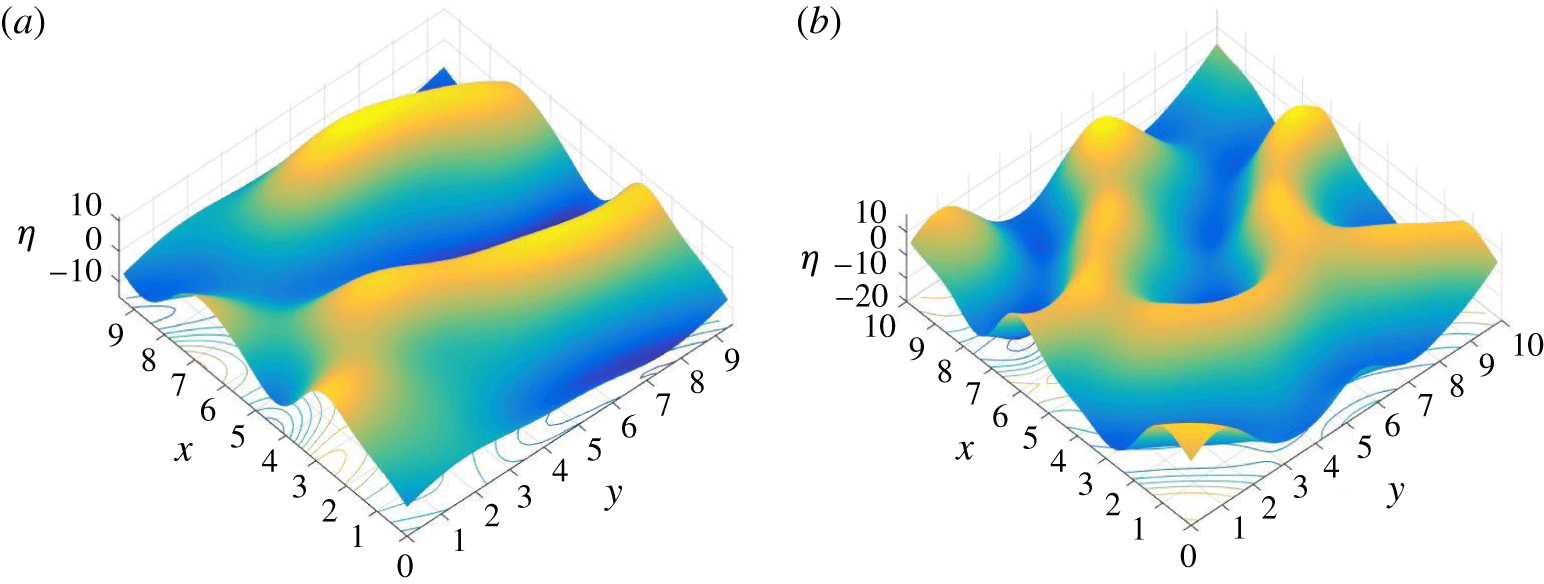
Figure 8. Representative profiles from the
 $A_{2}$
windows for
$A_{2}$
windows for
 $\unicode[STIX]{x1D6FD}=2$
. Panel (a) shows the profile of a travelling wave, and (b) a steady state in the
$\unicode[STIX]{x1D6FD}=2$
. Panel (a) shows the profile of a travelling wave, and (b) a steady state in the
 $A_{2}$
windows for the values of
$A_{2}$
windows for the values of
 $\unicode[STIX]{x1D6FE}=1.5$
and 2, respectively. The values of
$\unicode[STIX]{x1D6FE}=1.5$
and 2, respectively. The values of
 $L$
are 9.5 and 10.0, respectively.
$L$
are 9.5 and 10.0, respectively.
Finally, we briefly discuss the qualitative effect of introducing an electric field to a dynamical regime that is already chaotic. For chaos to arise in the absence of an electric field, we require a supercritical Reynolds number that already provides complex dynamics on periodic domains of sufficiently large lengths. We take
 $L=30$
so that chaotic dynamics is seen in the absence of a field, i.e.
$L=30$
so that chaotic dynamics is seen in the absence of a field, i.e.
 $\unicode[STIX]{x1D6FE}=0$
. Figure 9(a) shows a snapshot of the chaotic solution for this case, the interfacial profile remains strongly one-dimensional throughout the evolution. In the results depicted in figure 9(b–e), the electric field parameter is increased to
$\unicode[STIX]{x1D6FE}=0$
. Figure 9(a) shows a snapshot of the chaotic solution for this case, the interfacial profile remains strongly one-dimensional throughout the evolution. In the results depicted in figure 9(b–e), the electric field parameter is increased to
 $\unicode[STIX]{x1D6FE}=0.5$
, 1, 1.5 and 2, respectively. The flow remains chaotic as expected, and the snapshots shown indicate that the field has a crucial effect in introducing two-dimensionality into the interfacial fluctuations. The introduction of the field also increases the number of cellular structures, their amplitude, and the energy of the solutions defined by (4.31). A more complete presentation of the time evolution and dynamics of solutions in this regime can be found in supplementary movie 5. The movie is constructed by increasing
$\unicode[STIX]{x1D6FE}=0.5$
, 1, 1.5 and 2, respectively. The flow remains chaotic as expected, and the snapshots shown indicate that the field has a crucial effect in introducing two-dimensionality into the interfacial fluctuations. The introduction of the field also increases the number of cellular structures, their amplitude, and the energy of the solutions defined by (4.31). A more complete presentation of the time evolution and dynamics of solutions in this regime can be found in supplementary movie 5. The movie is constructed by increasing
 $\unicode[STIX]{x1D6FE}$
after intervals of 20 time units, explicitly we take
$\unicode[STIX]{x1D6FE}$
after intervals of 20 time units, explicitly we take
 $$\begin{eqnarray}\unicode[STIX]{x1D6FE}(t)=\left\{\begin{array}{@{}ll@{}}0\quad & \text{if }0\leqslant t<20,\\ 1\quad & \text{if }20\leqslant t<40,\\ 2\quad & \text{if }40\leqslant t<60.\end{array}\right.\end{eqnarray}$$
We find that a strengthening of the electric field increases the frequency of the chaotic oscillations of the energy
 $E(t)$
, as well as the amplitude of the solution (the average energy increases from approximately 40 to 100, and then to approximately 240, as
$E(t)$
, as well as the amplitude of the solution (the average energy increases from approximately 40 to 100, and then to approximately 240, as
 $\unicode[STIX]{x1D6FE}$
increases from 0 to 1, and finally to 2 as described above). In the interval
$\unicode[STIX]{x1D6FE}$
increases from 0 to 1, and finally to 2 as described above). In the interval
 $20\leqslant t<40$
, we observe approximately seven oscillations of
$20\leqslant t<40$
, we observe approximately seven oscillations of
 $E(t)$
, whereas increasing to
$E(t)$
, whereas increasing to
 $\unicode[STIX]{x1D6FE}=2$
in the interval
$\unicode[STIX]{x1D6FE}=2$
in the interval
 $40\leqslant t<60$
produces roughly 20 oscillations. These results show that even for supercritical Reynolds numbers where there is already instability in the
$40\leqslant t<60$
produces roughly 20 oscillations. These results show that even for supercritical Reynolds numbers where there is already instability in the
 $x$
-direction without an electric field effect, the transverse dynamics is non-trivial and not dominated by one-dimensional behaviour upon the introduction of the electric field.
$x$
-direction without an electric field effect, the transverse dynamics is non-trivial and not dominated by one-dimensional behaviour upon the introduction of the electric field.

Figure 9. Profiles of solutions in the chaotic regime for
 $\unicode[STIX]{x1D6FD}=2$
,
$\unicode[STIX]{x1D6FD}=2$
,
 $L=30.0$
.
$L=30.0$
.
5 Conclusions and future directions
We derived a long-wave Benney model (3.17) that describes three-dimensional long-wave dynamics of a gravity-driven thin film flow under the action of a normal electric field. For overlying films, the weakly nonlinear evolution is found to be governed by a Kuramoto–Sivashinsky equation (4.7) with a linear non-local term corresponding to the electric field. Solutions to this equation are bounded only if the electric field strength is below a threshold value – otherwise, unbounded exponential growth of the transverse modes cannot be prevented (as is the case for hanging films). The critical electric field strength is set by the condition that all purely transverse modes are linearly stable; mixed modes can still be unstable however, and hence produce non-trivial nonlinear two-dimensional phenomena. The present study has documented numerically a host of dynamical behaviours of solutions to (4.7) on periodic domains as the system size changes (a more in-depth study of the solution space is beyond the scope of the present work).
An important question to pose is, what happens when the electric field strength is above critical,
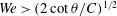 $We>(2\cot \unicode[STIX]{x1D703}/C)^{1/2}$
, and/or the film is hanging? In this case, the weakly nonlinear analysis breaks down (
$We>(2\cot \unicode[STIX]{x1D703}/C)^{1/2}$
, and/or the film is hanging? In this case, the weakly nonlinear analysis breaks down (
 $\unicode[STIX]{x1D702}$
does not remain
$\unicode[STIX]{x1D702}$
does not remain
 $O(1)$
), and hence we need to revert to the fully nonlinear Benney equation (3.17). Current work on this problem by the authors suggests that transverse structures form that are connected by thin film regions with dewetting being possible, for both hanging and overlying films – the results will be presented elsewhere. We have also tried to retain higher-order terms in the weakly nonlinear evolution in an effort to investigate whether structural stability can be attained with bounded solutions emerging. We find that this does not happen, and in fact, even more instabilities can enter, resulting in enhanced ill-posedness, something that is not unusual in gradient expansions. An additional direction with practical applications, involves using feedback control to stabilise the two-dimensional solutions either to the flat state or a predetermined non-uniform state. This is particularly interesting in parameter regimes where the model predicts unbounded growth. The authors are currently studying such control strategies, building on the one-dimensional work of Thompson et al. (Reference Thompson, Gomes, Pavliotis and Papageorgiou2016) and Gomes, Papageorgiou & Pavliotis (Reference Gomes, Papageorgiou and Pavliotis2017).
$O(1)$
), and hence we need to revert to the fully nonlinear Benney equation (3.17). Current work on this problem by the authors suggests that transverse structures form that are connected by thin film regions with dewetting being possible, for both hanging and overlying films – the results will be presented elsewhere. We have also tried to retain higher-order terms in the weakly nonlinear evolution in an effort to investigate whether structural stability can be attained with bounded solutions emerging. We find that this does not happen, and in fact, even more instabilities can enter, resulting in enhanced ill-posedness, something that is not unusual in gradient expansions. An additional direction with practical applications, involves using feedback control to stabilise the two-dimensional solutions either to the flat state or a predetermined non-uniform state. This is particularly interesting in parameter regimes where the model predicts unbounded growth. The authors are currently studying such control strategies, building on the one-dimensional work of Thompson et al. (Reference Thompson, Gomes, Pavliotis and Papageorgiou2016) and Gomes, Papageorgiou & Pavliotis (Reference Gomes, Papageorgiou and Pavliotis2017).
Finally, it is important to point out that (4.7) supports pattern formation phenomena and derives directly from an asymptotic analysis of the Navier–Stokes equations coupled with electrostatics. It is therefore of intrinsic interest as a pattern-forming two-dimensional evolution equation in analogous ways to the Swift–Hohenberg equation (Swift & Hohenberg Reference Swift and Hohenberg1977).
Acknowledgements
R.J.T. acknowledges the support of a PhD scholarship from EPSRC. The work of D.T.P. was supported by EPSRC grants EP/K041134 and EP/L020564, and the work of G.A.P. was supported by EPSRC grants EP/L020564, EP/L025159 and EP/L024926. We are grateful to R. Granero-Belinchón for his comments and a correction, and also to the referees for their extensive and useful comments and corrections.
Supplementary movies
Supplementary movies are available at https://doi.org/10.1017/jfm.2017.250.
Appendix A. Estimates for numerics
We now derive a condition on
 $c$
to ensure that the operator
$c$
to ensure that the operator
 ${\mathcal{A}}$
defined in (4.22a
) is positive definite on
${\mathcal{A}}$
defined in (4.22a
) is positive definite on
 $L^{2}$
. Firstly, by Cauchy–Schwarz and integration by parts,
$L^{2}$
. Firstly, by Cauchy–Schwarz and integration by parts,
 $$\begin{eqnarray}\displaystyle \langle {\mathcal{A}}\unicode[STIX]{x1D702},\unicode[STIX]{x1D702}\rangle _{2} & = & \displaystyle -(\unicode[STIX]{x1D6FD}-1)|\unicode[STIX]{x1D702}_{x}|_{2}^{2}+|\unicode[STIX]{x1D702}_{y}|_{2}^{2}+\unicode[STIX]{x1D6FE}\langle {\mathcal{R}}(\unicode[STIX]{x1D702}),\unicode[STIX]{x0394}\unicode[STIX]{x1D702}\rangle _{2}+|\unicode[STIX]{x0394}\unicode[STIX]{x1D702}|_{2}^{2}+c|\unicode[STIX]{x1D702}|_{2}^{2}\nonumber\\ \displaystyle & {\geqslant} & \displaystyle -\unicode[STIX]{x1D6FD}|\unicode[STIX]{x1D702}_{x}|_{2}^{2}-|\unicode[STIX]{x1D702}_{y}|_{2}^{2}-\unicode[STIX]{x1D6FE}|\unicode[STIX]{x0394}\unicode[STIX]{x1D702}|_{2}|{\mathcal{R}}(\unicode[STIX]{x1D702})|_{2}+{\textstyle \frac{1}{2}}|\unicode[STIX]{x0394}\unicode[STIX]{x1D702}|_{2}^{2}+\frac{1}{2}|\unicode[STIX]{x1D702}_{xx}|_{2}^{2}+{\textstyle \frac{1}{2}}|\unicode[STIX]{x1D702}_{yy}|_{2}^{2}+c|\unicode[STIX]{x1D702}|_{2}^{2}.\nonumber\\ \displaystyle & & \displaystyle\end{eqnarray}$$
From the Fourier symbol of
 ${\mathcal{R}}$
, it follows that
${\mathcal{R}}$
, it follows that
 $$\begin{eqnarray}|{\mathcal{R}}(\unicode[STIX]{x1D702})|_{2}=\sqrt{|\unicode[STIX]{x1D702}_{x}|_{2}^{2}+|\unicode[STIX]{x1D702}_{y}|_{2}^{2}}\leqslant |\unicode[STIX]{x1D702}_{x}|_{2}+|\unicode[STIX]{x1D702}_{y}|_{2},\end{eqnarray}$$
and Young’s inequality gives
 $$\begin{eqnarray}\displaystyle |\unicode[STIX]{x1D702}_{x}|_{2}^{2}\leqslant \frac{1}{2\unicode[STIX]{x1D716}_{1}}|\unicode[STIX]{x1D702}|_{2}^{2}+\frac{\unicode[STIX]{x1D716}_{1}}{2}|\unicode[STIX]{x1D702}_{xx}|_{2}^{2},\quad |\unicode[STIX]{x1D702}_{y}|_{2}^{2}\leqslant \frac{1}{2\unicode[STIX]{x1D716}_{2}}|\unicode[STIX]{x1D702}|_{2}^{2}+\frac{\unicode[STIX]{x1D716}_{2}}{2}|\unicode[STIX]{x1D702}_{yy}|_{2}^{2}, & & \displaystyle\end{eqnarray}$$
 $$\begin{eqnarray}\displaystyle \unicode[STIX]{x1D6FE}|\unicode[STIX]{x0394}\unicode[STIX]{x1D702}|_{2}|\unicode[STIX]{x1D702}_{x}|_{2}\leqslant \frac{\unicode[STIX]{x1D716}_{3}}{2}|\unicode[STIX]{x0394}\unicode[STIX]{x1D702}|_{2}^{2}+\frac{\unicode[STIX]{x1D6FE}^{2}}{2\unicode[STIX]{x1D716}_{3}}|\unicode[STIX]{x1D702}_{x}|_{2}^{2},\quad \unicode[STIX]{x1D6FE}|\unicode[STIX]{x0394}\unicode[STIX]{x1D702}|_{2}|\unicode[STIX]{x1D702}_{y}|_{2}\leqslant \frac{\unicode[STIX]{x1D716}_{4}}{2}|\unicode[STIX]{x0394}\unicode[STIX]{x1D702}|_{2}^{2}+\frac{\unicode[STIX]{x1D6FE}^{2}}{2\unicode[STIX]{x1D716}_{4}}|\unicode[STIX]{x1D702}_{y}|_{2}^{2},\qquad & & \displaystyle\end{eqnarray}$$
for any
 $\unicode[STIX]{x1D716}_{1},\unicode[STIX]{x1D716}_{2},\unicode[STIX]{x1D716}_{3},\unicode[STIX]{x1D716}_{4}>0$
. Then, using these with (A 1) yields
$\unicode[STIX]{x1D716}_{1},\unicode[STIX]{x1D716}_{2},\unicode[STIX]{x1D716}_{3},\unicode[STIX]{x1D716}_{4}>0$
. Then, using these with (A 1) yields
 $$\begin{eqnarray}\displaystyle \langle {\mathcal{A}}\unicode[STIX]{x1D702},\unicode[STIX]{x1D702}\rangle _{2} & {\geqslant} & \displaystyle \left(c-\frac{\unicode[STIX]{x1D6FD}}{2\unicode[STIX]{x1D716}_{1}}-\frac{1}{2\unicode[STIX]{x1D716}_{2}}-\frac{\unicode[STIX]{x1D6FE}^{2}}{4\unicode[STIX]{x1D716}_{1}\unicode[STIX]{x1D716}_{3}}-\frac{\unicode[STIX]{x1D6FE}^{2}}{4\unicode[STIX]{x1D716}_{2}\unicode[STIX]{x1D716}_{4}}\right)|\unicode[STIX]{x1D702}|_{2}^{2}+\left(\frac{1}{2}-\frac{\unicode[STIX]{x1D6FD}\unicode[STIX]{x1D716}_{1}}{2}-\frac{\unicode[STIX]{x1D6FE}^{2}\unicode[STIX]{x1D716}_{1}}{4\unicode[STIX]{x1D716}_{3}}\right)|\unicode[STIX]{x1D702}_{xx}|_{2}^{2}\nonumber\\ \displaystyle & & \displaystyle +\left(\frac{1}{2}-\frac{\unicode[STIX]{x1D716}_{2}}{2}-\frac{\unicode[STIX]{x1D6FE}^{2}\unicode[STIX]{x1D716}_{2}}{4\unicode[STIX]{x1D716}_{4}}\right)|\unicode[STIX]{x1D702}_{yy}|_{2}^{2}+\left(\frac{1}{2}-\frac{\unicode[STIX]{x1D716}_{3}}{2}-\frac{\unicode[STIX]{x1D716}_{4}}{2}\right)|\unicode[STIX]{x0394}\unicode[STIX]{x1D702}|_{2}^{2}.\end{eqnarray}$$
Taking
 $$\begin{eqnarray}\unicode[STIX]{x1D716}_{1}=\frac{1}{\unicode[STIX]{x1D6FD}+\unicode[STIX]{x1D6FE}^{2}},\quad \unicode[STIX]{x1D716}_{2}=\frac{1}{1+\unicode[STIX]{x1D6FE}^{2}},\quad \unicode[STIX]{x1D716}_{3}=\unicode[STIX]{x1D716}_{4}=\frac{1}{2},\end{eqnarray}$$
ensures that all the brackets preceding norms of derivative terms in (A 4) are zero. So to ensure that
 ${\mathcal{A}}$
is positive definite, it is sufficient to take
${\mathcal{A}}$
is positive definite, it is sufficient to take
 $$\begin{eqnarray}c>\frac{\unicode[STIX]{x1D6FD}}{2\unicode[STIX]{x1D716}_{1}}+\frac{1}{2\unicode[STIX]{x1D716}_{2}}+\frac{\unicode[STIX]{x1D6FE}^{2}}{4\unicode[STIX]{x1D716}_{1}\unicode[STIX]{x1D716}_{3}}+\frac{\unicode[STIX]{x1D6FE}^{2}}{4\unicode[STIX]{x1D716}_{2}\unicode[STIX]{x1D716}_{4}}=\frac{1}{2}[(\unicode[STIX]{x1D6FD}+\unicode[STIX]{x1D6FE}^{2})^{2}+(1+\unicode[STIX]{x1D6FE}^{2})^{2}].\end{eqnarray}$$


 Open access