


I. INTRODUCTION
A) Motivation
Digital media compression has been under development for decades, but it was only in the last years that its economic importance started to be comparable with other major economic activities, especially for video. This can be observed, for example on Cisco's annual Internet traffic report [1], which forecasts that global IP traffic will grow 2.75 times between 2016 and 2021, while “IP video traffic will be 82% of all consumer Internet traffic by 2021, up from 73% in 2016.”
While these numbers are already impressive, even faster growth is expected from new formats and applications. For instance, Cisco forecasts very large growth, during the same period, in live video (15×), and in virtual and augmented reality (80×). The resulting enormous bandwidth demands provide strong economic incentives for increasing the efficiency of media delivery, and since even small bandwidth reductions provide significant savings, there is now a continuous demand for better media compression.
Confirming this trend, a joint ITU-T and MPEG committee (JVET) started the process of developing a new standard, called Versatile Video Coding [Reference Chiariglione and Timmerer2], to replace the latest HEVC/H.265 video coding standard [Reference Wien3].
B) Research options
One difficulty in obtaining substantial bandwidth reductions comes from the fact that, since media compression is a relatively mature field, there are no “easy and cheap” ways left to significantly improve it, and the costs to develop better solutions have been growing.
As we consider how to improve media compression, we are faced with two main approaches:
(i) Fundamentally new media compression techniques;
(ii) Methods to improve the process of extending and developing known techniques.
While the first approach may seem risky, but possibly more promising, and the second being only evolutionary, the reality is somewhat more interesting. Actually, there are many techniques known to theoretically yield compression gains, but those were found to be very difficult to optimize and implement or to extend beyond simple cases. Some challenges are related to human limits, and part of the latest improvements in media compression came only after experts used their intuition and skills to painstakingly extend some well-known techniques.
This aspect can be better understood considering a specific case. It is well-known that video compression can be improved by using different types of classification and exploiting the statistical features of the data in each class. A common mistake is to first assume that we can exploit classification according to high-level human criteria, like people, faces, objects, etc. In reality, those are of little use for coding, and instead, we need low-level features, like identifying textures found in hair, grass, water, etc. Some of these low-level features are exploited by state-of-art coding methods, but they still tend to be related to human concepts (like geometric patterns, directional changes, etc.).
The reality is that we do not know if there are many other useful and possibly more powerful types of low-level features to exploit, which are not directly related to human concepts. Obviously, trying to use human intuition to find those features is not expected to be successful.
C) Why machine learning (ML)
As we look for approaches that can be employed for this type of problem, we can immediately find that tools developed under the general name of ML have been achieving extraordinary results solving similar problems in other applications, and wonder if they can be useful for compression too.
It is important to stress that this choice of ML is not gratuitous, or because the subject is now “trendy.” It is justified by the basic fact that, when we say we want to compress media, like movies or music, we do not have anything resembling a formal definition and mathematical model of what they are. Instead, what we really have is a very large set of examples, and this matches the basic “learning from examples” assumption now commonly used in ML.
For the same reason, it is also fair to say that several techniques that had been used for many years in media compression correspond to “new” ML tools, with the caveat that they were limited by the computer power available when they were first proposed.
This document is about the application of ML techniques for media compression. It is not meant to be a survey or an introduction to those subjects (found, e.g. in [Reference Mitchell4–Reference Marsland7] and [Reference Wien3,Reference Sayood8–Reference Woods10]), but is instead prepared to
• Help ML researchers find out how to modify their methods to make them suitable for media compression, and also to (hopefully) encourage the development of new techniques to solve some truly challenging coding problems.
• It is also addressed to media compression professionals who are trying to determine how machine learning can help achieve better results, especially when complementing or extending current coding techniques.
The examples are all related to video coding, but we believe the main ideas to be equally useful for other types of media.
We use the termML as a convenient way to refer to a large set of new technologies. From a practical side, ML tools are the result of the synergistic development of new theory and algorithms, matched to the availability of massive amounts of computational resources. This includes advances in completely new areas, like deep neural networks, to fast progress in traditional study fields, like statistics and optimization.
What we consider the distinguishing factors are:
• The assumption that large computational resources are going to routinely be employed;
• The “learning” tools can be used not only as problem solvers but to extend human knowledge, understanding, and help in the development of new techniques.
Thus, for convenience, we may call an optimization technique that was originally developed for, e.g. operations research, a “machine learning tool” if it is used within the context defined above.
Also, note that this definition is intentionally expanded to include humans as participating actors. For example ML can be combined with visualization, to first provide developers with insight, which is then turned into better solutions (this is further discussed in Section IV).
As explained in the next sections, this is one proposal for doing media compression using ML, and it is important to note that there are alternative strategies [Reference Toderici11,Reference Johnston12].
D) Some mistakes to avoid
Even if the advantages of combining the two fields may seem clear, we find it important to discuss some problems that have also delayed other multi-disciplinary efforts. For instance, it is common to observe (a) a temptation to look for quick solutions and underestimate the effort needed to create correct tools, and (b) when the results are disappointing, a tendency to quickly discard additional opportunities, and declare the whole endeavor a failure.
The problem is that media compression and ML have different traditions and cultures. For example, a significant part of media compression was developed using the approach of first creating certain explicit mathematical models, which are then used to reach conclusions and develop practical methods. When this is accepted as the “only correct” methodology, it can be preferred over equally powerful alternatives, even when there is a very clear mismatch between a model and actual examples. Conversely, if a technique is found to be extraordinarily successful in some “related” applications, it does not necessarily mean that it will be even useful for compression, and it is perfectly acceptable to refuse to trade it for “tried and true” methods, until more evidence is presented.
We argue that a better way to avoid these problems is as follows.
(i) First, identify the problem and not the solution, i.e. find what is the important compression problem that can potentially profit from ML, and avoid the “solution looking for a problem” approach.
(ii) Consider the broad picture, i.e. the concepts behind general ML strategies and tools, before trying particular solutions.
(iii) Fully adapt the approach to the compression problem, accepting the likelihood that a good amount of development is needed to match the performance of state-of-the-art codecs.
For instance, the question “Can we use deep neural networks (DNNs) for compression?” is certainly interesting by itself (assuming proper adaptation), but we believe an equally interesting question would be “Can the tools and general training techniques employed for designing DNNs also be effectively used for compression?”
Note that here we want to focus on the design process, and not the final product, considering for example, employing DNN design techniques to other computation structures. In Section III we present an actual example of such case – in the design of a new type of transforms for video coding, which have structure and purpose quite different from DNNs, but nevertheless share striking similarities in the design process.
E) Paper overview
In the next sections, we clarify and expand the concepts presented above, describing open problems, and also practical examples. It is important to note that, while some comments are about future research directions, the examples chosen actually improve the state-of-the-art video compression, while also satisfying practical complexity constraints. In fact, they have been accepted for inclusion on the latest MPEG/ITU-T test codec (JEM), used for evaluating technologies that can be part of the next video coding standard.
II. PREDICTION FOR MEDIA COMPRESSION
The use of statistical prediction provides a good example of why applying “off-the-shelf” ML tools for media compression is not as straightforward as it may initially seem. Figure 1 shows a general form of prediction studied in statistics and ML, including the components used during training. The design of good predictors, using a combination of mathematical models and training data is based on how well they optimize some measure of accuracy, plus considerations about computational complexity.

Fig. 1. A general prediction system, including the elements used for training.
The latest advances in the design of prediction systems have focused on the ability to develop increasingly more powerful and complex predictors, employing enormous amounts of training data. Since the results have been truly impressive, professionals working on media compression, and researchers studying ML, can observe that some of the most successful media compress systems employ prediction as a fundamental component, as shown in Fig. 2.
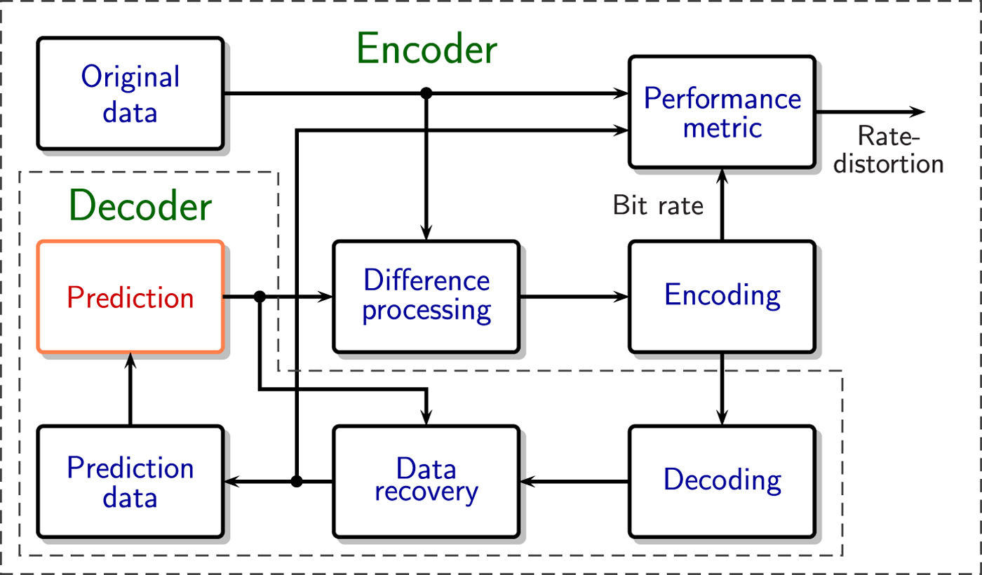
Fig. 2. A prediction-based system for lossy media compression.
Since the amount of compressed data is proportional to the average difference between the prediction and the true signal, we can assume that employing better prediction should improve compression. For example, a new type of predictor designed for video denoising and restoration may be useful for compression.
It is now very easy to employ one of the many ML software packages to train some predictors for images, and directly apply them to some form of prediction-based image compression. However, when the results turn out to be substantially worse than state-of-the-art, we can observe two opposite (and incorrect) interpretations:
• Those results are nevertheless “very promising” because they may possibly lead (in some yet unknown way) to novel and better ways to develop new compression methods.
• This “proves” that ML is mostly “hype,” and it cannot possibly compete with the well-established compression methods, which have been under development for decades.
The reality is that the experiment itself is wrong, i.e. there is a mismatch between the solution and the problem, and thus results are not necessarily meaningful.
The key to understanding the real problem is found from a more careful analysis of the system in Fig. 2, taking into account the fact that the encoder, differently from general-purpose prediction,
• Always has access to the original data;
• Contains the decoder as one sub-component.
These simple facts have profound implications in the choice and optimization of prediction methods, since the encoder can always compare the decoder output with the original data to make the most appropriate decisions.
This can be more easily observed by considering how to improve those two types of systems using a combination of different predictors. Figure 3(a) shows the case where the output of several predictors are combined, possibly using different weights derived from some measure of confidence. Since the original data are not available (except during training), there is no way to find which is the most accurate predictor, and the best we can do is find a combination method that, on average, improves the performance metric. Consequently, those predictors should be chosen and optimized to work in a cooperative way.

Fig. 3. Comparison of how (a) a general prediction system and (b) a prediction-based encoder, can use several prediction methods to improve performance. In the encoder, the residual is the difference between prediction and original signals.
The encoding system of Fig. 3(b), on the other hand, always has access to the original data, and it should be trivial to find which is the most accurate prediction. However, in this case, the most accurate is not always the best: since the encoder needs to add extra data to inform the decoder which predictor was used, it has to take that overhead into account, and use a rate-distortion (R-D) criterion to define which is the best prediction to use.
The importance of the prediction selection overhead should not be underestimated. For example, if two different predictors produce very similar results, combining the prediction does not change the accuracy, but selecting among the two only adds redundancy and degrades compression.
Additional examples of differences between the two types of application are
• The set of prediction methods for general prediction must have some measure of consistency and reliability to obtain a good combination, while the encoder can profit more from having diversity among the prediction methods.
• When the prediction outputs are vectors, a general predictor must use a combination function defined only by prediction data, while the encoder can use the original data to select from a broad class of functions, and explicitly send any type of side information (function selectors, parameters, etc.).
• Given the prediction data, in a working system the general prediction is unique, while the encoder's choice of best prediction may vary, since the R-D analysis depends on the user's desired R-D trade-off.
Of course, there are many other differences, but those examples should make clear that, even if the design of those two systems use similar tools, the objectives and results should be quite different.
Considering these factors, we can find a number of interesting research problems. For example, we can observe that a full encoder optimization should take into account the strong interdependence between the following factors.
(i) The encoder's method to select and possibly combine the best prediction (e.g. using linear combinations, type of side information, etc.);
(ii) The prediction techniques employed;
(iii) The parameters of each prediction method.
At this point, we have many solutions to optimize those elements independently, but we can also recognize that we can have much better solutions if they are optimized in a truly combined manner. In fact, similarly to the way that we can move from robots capable of doing only simple tasks, to more intelligent machines that adapt to their environment and tasks, we can envision using ML techniques to design more “intelligent encoders,” i.e. encoders which are capable of analyzing different media segments, and making intelligent decisions on which are the best tools to be employed for their compression.
Note that here prediction was used just to exemplify one case. Similar conclusions are also valid for other compression techniques. For example, transform coding applied to compression is similar to principal component analysis applied for ML, but we again have fundamental differences regarding their application.
III. ADDING TRANSFORMS
Media coding systems based on prediction also exploit the fact that commonly there is statistical dependence left in the components of the difference between prediction and original signals (the residual), and better compression is obtained when the residual goes through a linear transformation to decorrelate its elements, before coding.Footnote 1 For example, different forms of the discrete cosine transform have been used for this purpose on video, image, and audio coding.
Up to now video coding standards have not been too different from what is shown in Fig. 3(b), using basically only one type of transform for the residual. However, compression is improved if we use some form of classification, and employ transforms matched to the statistics of the residuals in each class [Reference Han, Saxena, Melkote and Rose13], and this property already started to be exploited in video coding standards [Reference Sullivan, Ohm, Han and Wiegand14,Reference Mukherjee15]. In this section, we consider how to extend this approach.
Figure 4 shows such an encoder which not only selects from multiple prediction methods, but also exploits the fact that different predictors create residuals with specific statistical properties, and chooses among different transforms optimized for each prediction method. (Here classification is done through the choice of predictor, but more general approaches are possible.)
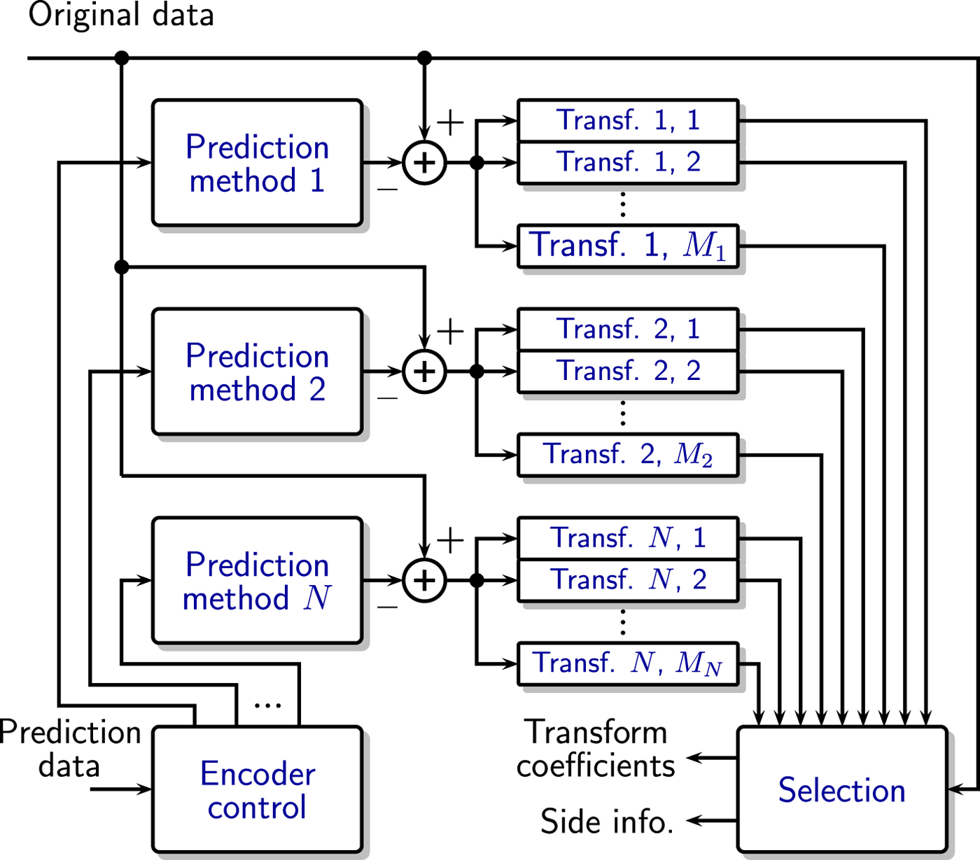
Fig. 4. Inclusion of multiple transform options to the encoder of Fig. 3(b).
When designing the encoder of Fig. 4, we are faced with two main practical problems:
(i) Identify and optimize the transform set for each prediction method.
(ii) Minimize the computational complexity required by the transforms.
Since the first objective is directly related to signal statistics, it should be clear that it should profit from ML techniques. In fact, many of the comments applied to prediction in the previous section are also valid here, and those techniques can be found in several new techniques (e.g. [Reference Sezer, Harmanci and Guleryuz16–Reference La, Xu, Zeng, Shi and Wu19]).
The second objective is very important in practice because high computational complexity is the main reason multi-transform systems have not been widely adopted. We consider it in this section, since it is a good example of a media compression problem which may seem completely unrelated to ML, but in fact shares important features, and can use its newly developed tools.
The problem we are considering can be easily stated: for video coding, if we have M T non-separable transforms that can be applied to 2k×2k two-dimensional blocks of prediction residuals, the complexity of operations per transform is O(24k), and the memory for all transform matrices has complexity O(24k M T).
This fast exponential growth means that those transforms can only be used for relatively small block sizes. However, even for those cases, we still need a relatively large number of transforms [Reference Zhao, Chen, Said, Seregin, Eğilmez and Karczewicz20], and memory requirements become a problem.
Transform coding has similarities to the principal component analysis technique used in ML, but the caveat is that for compression we cannot optimally predefine a number of components to maintain and to ignore since that number depends on the desired reproduction quality. Thus, the common approach is to have the encoder compute all components, and then use R-D to decide which should be used.
A new solution proposed for the transform complexity problem [Reference Said, Zhao, Karczewicz, Eğilmez, Seregin and Chen21] exploits the fact that compression gains are normally defined by signals in certain low-dimensional subspaces – which are in a sense “the principal” components and thus need a specific representation – but there is a great degree of freedom for representing the signals in the remaining space.
Using this property, we can impose a low-complexity implementation on the transform, called parametric multi-pass transform. Fig. 5 shows the main concept: instead of implementing the N-dimensional transform using an N×N matrix, it is computed in a series of P passes, each with computational complexity O(N).
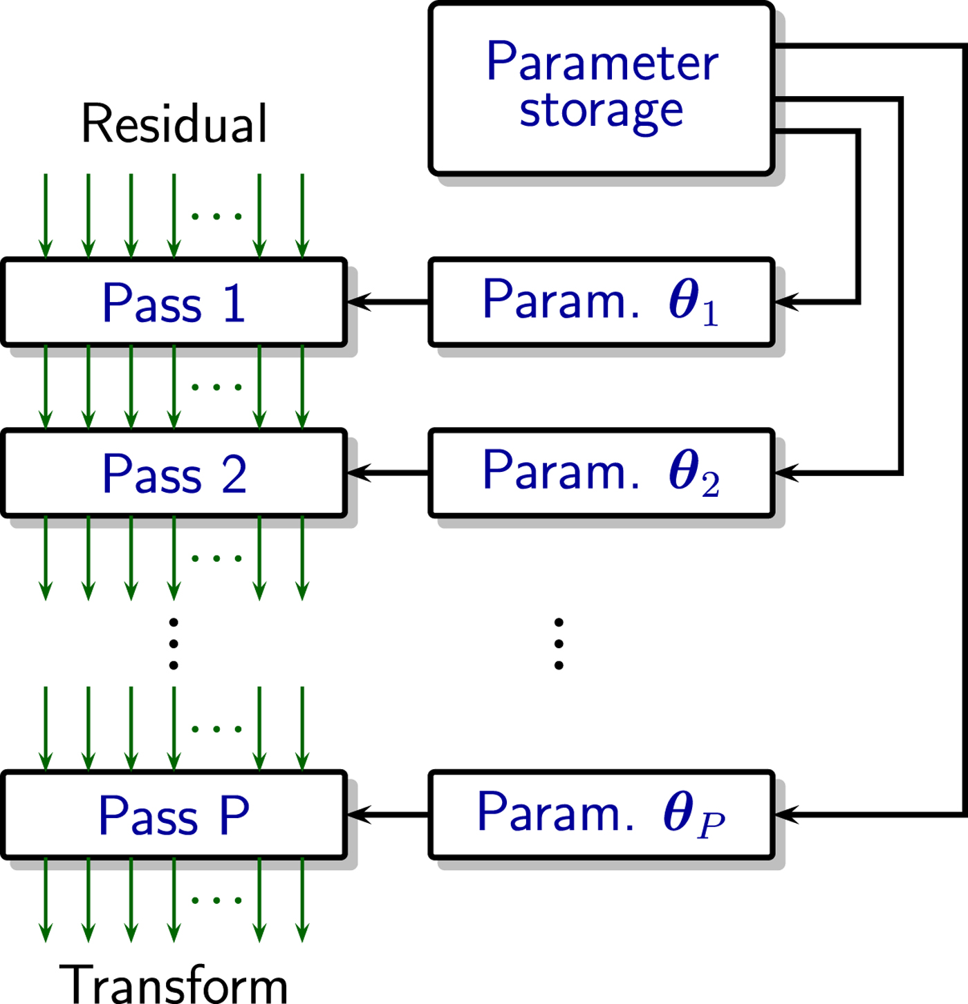
Fig. 5. Parametric multi-pass transform of dimension N: the computational complexity (memory and operations) in each pass is O(N).
The implementation tested was done using N/2 parallel Givens rotations in each pass, but here we do not need to go into those details, which are available in the original reference [Reference Said, Zhao, Karczewicz, Eğilmez, Seregin and Chen21].
What is interesting to discuss is the fact that, while the traditional transform optimization is based on the well-known concept of matrix diagonalization, the new implementation requires new solution methods. The conventional approach to finding a solution would be
(i) define a mathematical model for the data;
(ii) use it to develop closed-form solution methods;
(iii) test how well results fit practical data.
The approach used by some ML techniques, like neural networks [Reference Hagan, Demuth, Beale and De Jesús22], is to recognize that we can start from a parametric computation structure, and optimize it using training data.
For instance, in our transform design, the solution is completely defined by arrays of rotation angles (transform parameters), which we can always test on sets of training videos to see how well it performs. Of course, this requires a good amount of computational resources, but as mentioned in the introduction, this is now considered an integral part of the design process.
If we consider the problem from this perspective, we can observe that transforms and neural networksFootnote 2 have quite different processing elements, but share many design similarities, as listed in Table 1 and Fig. 6.
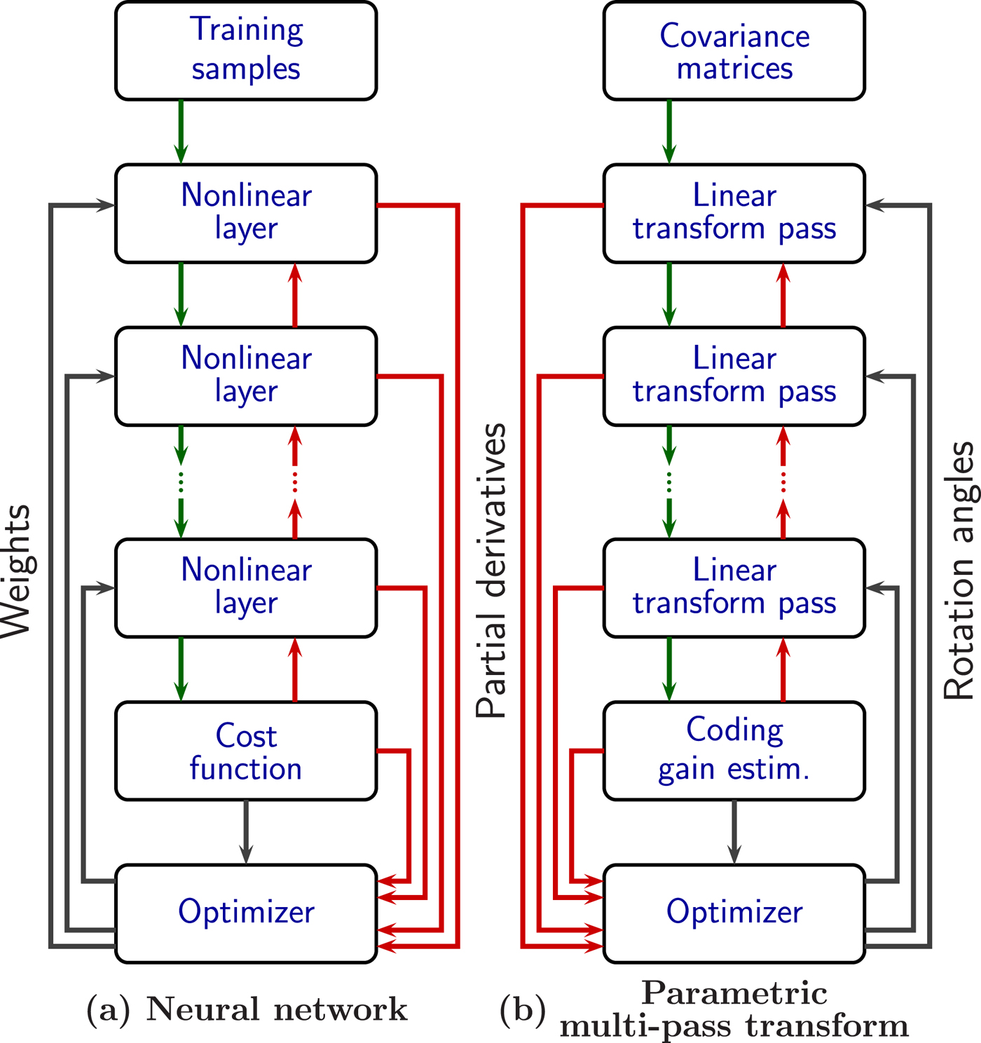
Fig. 6. Similar optimization (learning) structures of neural networks and parametric multi-pass transform. Green arrows represent processed data, and red arrows represent partial derivatives.
Table 1. Comparison of features of Neural Networks (NN) and Parametric Multi-Pass Transforms (PMPT)

The most fundamental similarity is the fact that the desired design is not defined by any mathematical model of the data, but instead from
(i) a basic computational element (e.g. neuron or Givens rotation);
(ii) a performance metric;
(iii) training data (preferably large amounts of).
Resulting from this we have the other elements that are shared, like using a gradient-based optimization, which in turn can employ back-propagation, which may require large computational resources, etc.
From those observations, we can look for more opportunities to get inspiration for new design techniques and learn about useful developments in other areas. For example, both designs can profit from advances in the very general area of automatic differentiation [Reference Bartholomew-Biggs, Brown, Christianson and Dixon23,Reference Griewank24], for faster development of algorithms for parameter optimization.
The results in [Reference Said, Zhao, Karczewicz, Eğilmez, Seregin and Chen21] show that using these techniques for video compression, it was possible to reduce memory requirements for transform parameters by factors of 5-7, with negligible losses in coding gains.
IV. HUMAN PARTICIPATION
Since ML is frequently used to develop methods to minimize or eliminate the need for human intervention, this sometimes is confused with one of its main objectives. However, ML tools are also very useful if we assume some degree of human participation, which frequently becomes much more efficient with the use of visualization tools.
To demonstrate this, here we present one example based on the intra-frame prediction of the HEVC/H.265 video compression [Reference Wien3], but discussed at a level that can also be understood by non-experts. The encoder is basically the system shown in Fig. 3, where data to be predicted are the pixels in the rectangular block, and the prediction data are composed of a subset of the pixels from previously coded blocks (called reference pixels).
There are 33 directional linear predictors, which simply assume that pixel values are nearly constant (or vary less) along a given direction. The way proposed in [Reference Said, Zhao, Karczewicz, Chen and Zou25] to visualize how the different directional predictors work is shown in Fig. 7(a). The gray values in each square represent the magnitude of the prediction coefficients, for a given reference pixel, to pixels in an 8×8 block being predicted, with gray equal to 0, white equal to 1, and black to –1. Reference pixels vary along the rows of blocks, and directional mode along the columns.
Fig. 7. Examples of how a visualization tool for prediction can lead to the design of better predictors. (a) represents the original “human based” design, (b) the ML design, but without complexity taken into account, and (c) is the “mixed” low-complexity design, with a model inspired on the predictors visually observed in (b), and ML for parameter optimization.
For example, the row of blocks with vertical white lines (near the center of the image) corresponds to the vertical prediction mode, which uses the pixel value at the top of the block as the prediction to all pixels under it. Since those are 8×8 blocks, we observe 8 vertical lines. The other rows correspond to other directional predictors, so all the lines have the same slope.
Understanding all the factors in those images may not be easy at first, but the important fact to keep in mind is that it is a way to completely represent visually everything about the directional predictors. We can observe that they are obviously a “human-based” design since it is completely defined by geometric ideas.
Figure 7(b) shows a set of similar directional predictors, but those were designed by training, using one of the many ML techniques available for that purpose [Reference Lucas, da Silva, de Faria, Rodrigues and Pagliari26]. We can notice that due to the variability found during training, it is noisier and the lines appear blurred. Nevertheless, since those predictors have been optimized for real videos, the experimental tests show that they clearly produce better prediction, and improved compression.
The only practical problem with the predictors of Fig. 7(b) is that they have a computational complexity that is too high for video coding applications. In fact, there are many interesting research problems related to the optimal design of predictors, using training, which fully includes computational complexity constraints, but those are still unsolved (cf. Section V).
Instead of waiting for better automatic tools to be developed, a designer still can use Fig. 7(b) to visually identify what are the modifications needed to improve compression. This approach was used [Reference Said, Zhao, Karczewicz, Chen and Zou25] to design some low-complexity modifications to the predictors of Fig. 7(a) in order to reproduce the main features observed in Fig. 7(b), and with approximation parameters optimized by training.
The image corresponding to those new predictors is shown in Fig. 7(c). We can visually observe that Fig. 7(c) is certainly more similar to Fig. 7(b), and the experimental results show that, while compression is not as good as with the high-complexity predictors, it is significantly better than the original directional predictors.
Visualization is also very useful for identifying when ML tools are producing incorrect results. For example, while computing the predictors shown in Fig. 7(b), among hundreds of cases where the correct type of directional prediction appear, the patterns of Fig. 8 also appeared.
Fig. 8. Examples of how repeated video parts can produce very severe over-fitting of predictors.
What they show is the common ML problem of predictor over-fitting, which can be very severe in media applications, because the same data patterns can appear many times, and bias the training. What is seen in Fig. 8 occurred because a single video sequence with constant background was accidentally included in the training set. The repeated use of the same pattern during training dominated over the desired pattern and resulted in predictors that are finely tuned to those repetitions. Visualization enabled quickly finding the problem among hundreds of predictors.
V. RESEARCH PROBLEMS
The examples in the previous sections provide some evidence that ML techniques can indeed help improve media compression, sometimes in unexpected ways, since they can also be used to create new coding algorithms, computation methods, etc. Note that in those cases, the key aspect is that the compression problem was defined first, and then the suitable solution techniques were identified.
Those are simple examples for which some answers are known, to show the potential of ML. However, they also contain several interesting and challenging research problems, which are not discussed here, because they are outside the scope of this paper.
In this section, we provide a brief discussion of some of those research problems.
Training process decomposition
Optimizing compression parameters can be as simple as shown in Fig. 9(a), where an optimization method iterates over the training media, and uses sets of R-D results to find the optimal solution. This can be more complicated when we have very large volumes of training data (to avoid the over-fitting problems), but there are ML techniques designed for very large data sets.
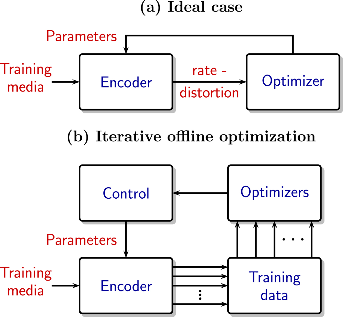
Fig. 9. Using training media for codec parameter optimization: (a) direct optimization, and (b) offline optimization needed when encoder complexity and data volumes are too large.
For media compression, we have the additional problem that the encoder can have very high complexity. In ML terms, besides large volumes of training data, we can also have a cost function that has very complex behavior and is extremely expensive to compute.
One solution commonly used for those cases is to first add functions to save some of the encoder's internal states, and the data that is affected by the parameters being optimized, and then decompose the optimization problem into a number of subproblems, which can be solved much more efficiently. The partial solutions are then aggregated into new parameters, and the process is repeated, as shown in the system of Fig. 9(b).
This “decompose and iterate until it hopefully converges” approach has been successfully used many times, but it can also fail terribly. This can be caused by the mathematical properties of the problem, but with media compression, where the encoder makes many decisions based on media characteristics (i.e. it contains many adaptive components), it can fail due to many other reasons related to the training media, like training subsets with very few cases and overfitting.
For instance, if at one iteration predictors become over-fitted (like those on Fig. 8), at the next iteration an adaptive encoder may assign a high overhead to its selection, and make the over-fitting worse. This, in turn, causes the optimization algorithm to diverge.
Part of the solution is related to training media selection, which is discussed next, but it also shows the need for more research on techniques that can make parameter optimization via training more reliable.
Training data selection
Collecting training data for media compression is a complicated task because:
• Commonly the data may not be composed of actual media samples (as when optimizing transforms for video residuals), and for that reason, the media itself cannot be composed of small segments, like a few frames of video, or milliseconds of music. It may be necessary to bring the encoder to some typical “steady state,” before starting data collection.
• It can be desirable to use the same codec for different media features, which can range from quality choices to media representation, like sample bit precision, video resolution and frame rates, audio sampling rates, etc.
• There are media types that can only be defined in a subjective manner, like action movies and video conferences, or music and voice only, etc.
For those reasons, human intervention is definitely needed while selecting the training data. However, there are some “low level” aspects that are difficult for people to control, and can profit from new research:
• When all the distinct data types and quality settings are put together for training, some cases can create much larger amounts of data than others. If all the data is aggregated, then the training will be over-fitted to those special cases. Thus, it is desirable to see new techniques to automatically compute the correct “weights” for the different data elements, so that training is not biased by the data volume.
• Related to the previous case, training can be an expensive and time-consuming task, and it can be ruined if there is over-fitting. Techniques for identifying the risk of over-fitting before or during training would greatly help.
Classification and data partitioning
When considering an encoding system as shown in Fig. 4, a question that immediately comes to mind is how to find the optimal set of predictors and of transforms. There are several approaches that have worked in practice, but many are ad hoc.
One common practice is to start from intuitive concepts, like geometry, rhythm, etc., and then try improving the initial solution. However, this sometimes fails in ways that are hard to understand. Another alternative is to start from several sets of random solutions, apply some refinement techniques, and then choose the best.
While those approaches do work in practice, when the solution is not well understood, it leaves designers with a difficult task of justifying why it should be used. The explanation that “it works, but we don't know exactly why,” is not acceptable when there are large investments involved.
Thus, it is desirable to have better methodologies to make the design process more reliable and develop tools for a better analysis of the factors involved.
This aspect is also related to the discussion of when to use ML for exploitation, i.e. improving known techniques, and exploration, when it helps find previously unknown facts. Researchers tend to be much more comfortable with the former since the latter is considered one thing humans do better.
From the previous discussions, it should be clear that our position is that the most exciting research is in using ML for exploration and discovery, not necessarily without human intervention, but intentionally searching for what is beyond human capabilities. However, as explained above, it is highly desirable to have tools that help designers understand why one solution is truly the best.
CONCLUSIONS
Due to the growing economic importance of media compression, there is now a constant demand for bandwidth reduction via better compression, and it is necessary to identify new approaches for improving media coding.
This paper addresses the possibility of using novel ML techniques to extend current coding techniques in completely new ways. For that purpose, it uses a very broad definition of ML, to include techniques developed in many fields of study, like statistics, optimization, and computation. It also assumes that human interaction, and techniques like visualization, can further improve the development of new compression techniques.
From this point of view, ML can be used to denote techniques from several scientific fields. In other words, it is like a “bazaar” where it is possible to find many new developments, including some that can turn out to be quite useful for media compression. However, those are more commonly in the form of general ideas and techniques, than ready-to-use solutions, and additional research and development is needed to find the best matches.
Thus, the first aspect analyzed was the observation that advanced media compression, i.e. the type needed for going beyond the state-of-the-art has very specific characteristics and needs, and it does not make sense to use, without proper adaptation, ML methods developed for other applications. Failure to recognize what is truly needed leads to disappointing results and backlash.
This point is first exemplified by showing how the use of prediction in general applications and in media compression may initially seem very similar, but, in fact, there are fundamental difference, which requires using quite distinct design methods. The second case considered is meant to show how, in trying to find a better practical solution to a classical coding problem (signal-dependent transforms), we find a problem that has many similarities with the design of neural networks, and thus profits from using very similar solution techniques.
The next case considered, the design of predictors for video coding, was chosen to illustrate how ML (which is frequently considered as a way to remove human participation) can be used together with visualization, to find non-intuitive patterns, which in turn helps designers to create better solutions.
Following those examples, a list of research problems is presented. They cover a very small range of cases but show that work in this area is just beginning, and there are very interesting possibilities. What we can expect is that in the future, we will have truly intelligent coding methods, that can identify properties of the media that are not related to common human concepts, but that can be effectively exploited for better compression.
A) Disclaimer
The views and opinions expressed in this article are those of the author, and may not necessarily reflect the official positions of his current or past employers.
Amir Said received the B.S. and M.S. degrees in electrical engineering from the University of Campinas, Brazil, and the Ph.D. degree in Computer and Systems Engineering from the Rensselaer Polytechnic Institute, Troy, NY, USA. His current research interests are in the areas of multimedia signal processing, video compression, and machine learning. He has more than 100 published technical papers, and 60 patents and applications, with more than 12000 citations on Google Scholar. He received several awards including the Allen B. DuMont prize from the Rensselaer Polytechnic Institute; a Best Paper Award from the IEEE Circuits and Systems Society for his work on image coding, the IEEE Signal Processing Society Best Paper Award for his work on multi-dimensional signal processing, and a Most Innovative Paper Award at the 2006 IEEE ICIP. Among his technical activities, he was Associate Editor for the SPIE/IS&T Journal of Electronic Imaging, and for the IEEE Transactions on Image Processing. He was a member of the IEEE SPS Image, Video, and Multidimensional Signal Processing Technical Committee, was technical co-chair of the 2009 IEEE Workshop on Multimedia Signal Processing, and has co-chaired VCIP, IVCP and VIPC conferences at the SPIE/IS&T Electronic Imaging from 2006 to 2015. Dr. Said is a fellow of the IEEE.


 Open access