


1. Introduction
Acoustic streaming is a stationary (time-independent) flow occurring in fluids (gases or liquids) subjected to a high-intensity sound field (Nyborg Reference Nyborg1998). Such flow is obtained without any external mechanical contact, which is a real advantage for the manufacture of either delicate or aggressive materials, as in the crystal growth from a melt where the stirring of the liquid during the solidification is needed to homogenize the impurities (Oh, Park & Cho Reference Oh, Park and Cho2002; Kozhemyakin Reference Kozhemyakin2003; Kozhemyakin, Nemets & Bulankina Reference Kozhemyakin, Nemets and Bulankina2014; Eskin Reference Eskin2015). Acoustic streaming is also relevant to other industrial applications such as the pumping of fluids (Rudenko & Sukhorukov Reference Rudenko and Sukhorukov1998), sometimes in microflow systems (Frampton, Martin & Minor Reference Frampton, Martin and Minor2003), the mixing of liquids in closed containers (Suri et al. Reference Suri, Takenaka, Yanagida, Kojima and Koyama2002) or the enhancement of rate-limited processes such as diffusion, or heat and mass transfer (El Ghani et al. Reference El Ghani, Miralles, Botton, Henry, Ben Hadid, Ter-Ovanessian and Marcelin2021).
This streaming is a nonlinear effect which can be connected to the Reynolds stresses associated with the rapidly oscillating acoustic velocities, but necessitates the dissipation of the acoustic energy flux (Lighthill Reference Lighthill1978; Nyborg Reference Nyborg1998; Moudjed et al. Reference Moudjed, Botton, Henry, Ben Hadid and Garandet2014). This dissipation could be due to the presence of boundaries and occurs in the acoustic boundary layers. The flow thus generated is called Rayleigh–Schlichting streaming. The dissipation could also be related to the attenuation of the wave in the fluid bulk and, in this case, it generates Eckart streaming. For the Eckart streaming considered here, the fluid flows away from the ultrasound source in the same direction as the ultrasound wave propagation.
The use of acoustic streaming in crystal growth applications induces its interaction with temperature gradients, heat transfer phenomena and gravity induced convective flows (in such heated situations the Prandtl number ( ${\textit {Pr}}=\nu /\kappa$, where
  $\nu$ is the kinematic viscosity and
  $\kappa$ is the thermal diffusivity) appears as a non-dimensional characteristic parameter for the system). Only few studies have treated such interactions. Vainshtein, Fichman & Gutfinger (Reference Vainshtein, Fichman and Gutfinger1995) analytically investigated the effect of Rayleigh–Schlichting streaming on the heat transferred between two horizontal parallel plates kept at different temperatures (hot plate above). They found a marked enhancement of the heat transfer due to the Rayleigh–Schlichting streaming and derived asymptotic relations expressing the mean Nusselt number variations. Hyun, Lee & Loh (Reference Hyun, Lee and Loh2005) performed experimental and numerical studies to measure the enhancement of the convective heat transfer due to acoustic streaming induced by a vibrating beam (Rayleigh–Schlichting streaming). For a heat transfer from above, the vibrations induce a temperature drop, which increases with the vibration amplitude, and is enhanced when the gap is open rather than closed. Their numerical calculations are able to reproduce the acoustic streaming flow and quantitatively confirm the drop in the temperature observed when the acoustic vibrations are applied. More recently, Green et al. (Reference Green, Marshall, Ma and Wu2016) experimentally studied the flow created by a vertically oriented ultrasonic transducer, placed at the top endwall of a cylindrical Pyrex container. The bottom endwall is an absorbing material, which will be progressively heated by the absorbed impinging acoustic beam. They show that a quasi-steady flow field driven by acoustic streaming is rapidly established within the container, but that this flow, after some time, is transformed into a secondary flow state, due to a thermal instability induced by the progressively heated bottom.
Some other studies considered the heat transfer in air between a lower hot plate and an upper cold plate, but in the case of acoustic standing waves for which only Rayleigh–Schlichting streaming is effective. Nabavi, Siddiqui & Dargahi (Reference Nabavi, Siddiqui and Dargahi2008) experimentally studied the modifications induced in the streaming velocity fields by such differentially heated horizontal walls. They found that, when the temperature difference is increased, the streaming velocities are increased too and the originally symmetric streaming vortices are deformed to give asymmetric vortices. Aktas & Ozgumus (Reference Aktas and Ozgumus2010) numerically studied a similar configuration with a two-dimensional approximation. They point out that the transverse temperature gradient strongly affects the acoustic streaming structures and velocities. They also mention an enhancement of the overall heat transfer due to the acoustic streaming.
Finally, some studies considered the influence of Eckart streaming on the flow and instabilities induced in differentially heated cavities. In the case of a side-heated cavity, a situation often referred to as the horizontal Bridgman configuration in the field of crystal growth, Dridi, Henry & Ben Hadid (Reference Dridi, Henry and Ben Hadid2008a) first considered a three-dimensional cavity where the streaming was induced by a transducer of fixed square shape generating an acoustic beam along the long horizontal axis of the cavity. For varying aspect ratio, acoustic intensity and Prandtl number, they show how the convective flow is modified by the streaming and how the further transitions at bifurcation points are also influenced. Dridi, Henry & Ben Hadid (Reference Dridi, Henry and Ben Hadid2010) then considered an infinite layer submitted to a horizontal temperature gradient and to acoustic streaming induced by a horizontal ultrasound beam. In the framework of the parallel flow approximation, they first determine analytically how the cubic profile of the convective flow is modified by the streaming, for different widths and positions of the acoustic beam. In a second step, they study the transition to instabilities, first for pure streaming flows, and then for convective flows submitted to streaming. They show how the instability thresholds are modified, depending on the type of instability, the Prandtl number, the position of the beam and the acoustic intensity. Finally, Ben Hadid et al. (Reference Ben Hadid, Dridi, Botton, Moudjed and Henry2012) studied the influence of Eckart streaming on an infinite layer heated from below (Rayleigh–Bénard configuration), in the case of a horizontal centred acoustic beam. They show how the transition to instability is modified by the streaming, with a threshold evolving in a continuous way from the Rayleigh–Bénard threshold to the pure streaming threshold. Depending on the beam width and the Prandtl number, stabilization of the Rayleigh–Bénard flow by the streaming can be obtained, with an increase of the thresholds (instability onsets) by a factor of up to 10.
The Rayleigh–Bénard configuration will still be considered here. It is a prototype configuration for flow transitions and heat transfer purposes, which has been studied extensively. The influence of Eckart streaming on such a configuration is a general theoretical issue, but it could also be interesting for different applications such as crystal growth, heat transfer between plates and Soret separation devices (Charrier-Mojtabi, Fontaine & Mojtabi Reference Charrier-Mojtabi, Fontaine and Mojtabi2012; Charrier-Mojtabi et al. Reference Charrier-Mojtabi, Jacob, Dochy and Mojtabi2019). In an infinitely extended fluid layer, the onset of the flow in the Rayleigh–Bénard configuration occurs through an instability at a critical value of the Rayleigh number,  ${\textit {Ra}}_c=1707.762$, with a critical wavenumber,
  $\alpha _c=3.117$. We will consider here a two-dimensional cavity with an aspect ratio
  $A_y={\rm length}/{\rm height}=10$, which corresponds to a slight confinement in the longitudinal
  $y$ direction compared with the extended layer, and the streaming will be induced by an acoustic beam of characteristic dimensionless size
  $H_b=h_b/h=0.338$, where
  $h$ is the height of the cavity and
  $h_b$ is the size of the beam. As shown in Ben Hadid et al. (Reference Ben Hadid, Dridi, Botton, Moudjed and Henry2012), the determination of
  $H_b$, in practice the width of the gate function corresponding to the applied force, is not so simple when considering a grid where the function cannot evolve sharply, but can only move from 1 to 0 on neighbouring points. To match with the analytical velocity profiles obtained in extended layers, it was found that
  $H_b$ has to be calculated as
  $(x(n_u)+x(n_u+1))/2-(x(n_d)+x(n_d-1))/2$, where
  $n_d$ and
  $n_u$ are the extreme points where the force is applied, this force going to 0 at
  $n_d-1$ and
  $n_u+1$, and
  $x$ is the dimensionless vertical coordinate at these points, ranging from
  $-0.5$ to
  $0.5$. On our mesh with 87 points along the vertical, the force is applied on 9 points on both sides of the horizontal axis, from
  $x(n_d) \approx -0.1605$ to
  $x(n_u) \approx 0.1605$. With
  $x(n_d-1) \approx -0.1775$ and
  $x(n_u+1) \approx 0.1775$, we obtain
  $H_b \approx 0.338$.
In this study, we will first focus on the modifications the Eckart flow induced by acoustic streaming is able to introduce in the stability of the Rayleigh–Bénard problem in such a cavity, in particular the modification of the thresholds and the change of instabilities. In a second step, we will characterize the flows, steady or oscillatory, which develop beyond these thresholds. This problem has similarities with the Poiseuille–Rayleigh–Bénard situation (Nicolas Reference Nicolas2002). Interestingly, the Eckart streaming in the closed cavity generates both flows in the beam direction along the beam axis and in the opposite direction along the boundaries, whereas the Poiseuille flow has only one direction, namely the direction induced by the imposed pressure gradient. We will see that very interesting behaviours will be put into light in our configuration. To tackle this problem, a spectral element code is used allowing time evolution calculations, the continuation of steady solutions and bifurcation points, but also the continuation of periodic oscillatory solutions. The combination of these different tools is a key element of this study.
After the introduction, we present the governing equations of the problem and the derivation of energy budgets in § 2. The numerical methods are shortly described in § 3 with tests of accuracy. The results concerning streaming flows without buoyancy are presented in § 4. The influence of these streaming flows on the buoyant instability thresholds is depicted in § 5. What occurs beyond these thresholds is described in §§ 6 and 7. After the presentation of the forward and backward waves in § 6, we describe the more global dynamics involving competition between steady solutions and waves in § 7.
2. Governing equations and energy budgets
2.1. Governing equations
We consider a rectangular cavity of height  $h$ along
  $x$ and length
  $l$ along
  $y$ (aspect ratio
  $A_y=l/h$) filled with a homogeneous Newtonian fluid and subject to a vertical temperature gradient and to the effect of ultrasound waves (see figure 1). The vertical temperature gradient is due to differentially heated horizontal walls. The waves are generated by an ultrasound source, of size
  $h_b$ (
 $h_b< h$), located in the middle of the left endwall of the cavity. The right endwall is assumed to be absorbing for sound waves so that reflection is avoided and the waves propagate in the horizontal
  $y$ direction, towards the right. The physical model is the one already used by Ben Hadid et al. (Reference Ben Hadid, Dridi, Botton, Moudjed and Henry2012). The previous study, however, considered a cavity with an infinite length and focused on the stability thresholds.

Figure 1. Sketch of the studied configuration. The rectangular cavity has an aspect ratio  $A_y=10$. The horizontal walls are isothermal: the bottom wall (in red) is at a hot temperature
  $T_h$, whereas the top wall (in blue) is at a colder temperature
  $T_c$. The lateral walls (in black) are adiabatic. All the boundaries are rigid walls with no-slip conditions. An acoustic wave is emitted by a transducer on the left wall and absorbed by an absorber at the right wall. It generates streaming taken into account through a body force
  $F$ considered as a gate function on the beam width (dashed lines).
The attenuation of the wave inside the fluid generates a body force. As shown by Nyborg (Reference Nyborg1998), this force is equal to the spatial variation of the Reynolds stress and can be written as  $F= -\rho \langle (u' \boldsymbol {\cdot } \boldsymbol {\nabla })u' +u' (\boldsymbol {\nabla } \boldsymbol {\cdot } u') \rangle$, where
  $\rho$ is the constant equilibrium density,
  $u'$ is the fluctuating velocity in the sound wave and
  $\langle \,\rangle$ means a time average over a large number of cycles. For a plane wave propagating in the
  $y$ direction, this body force is oriented in the
  $y$ direction and its intensity is given by
  $F= \rho \gamma V_a^2 \, {\rm e}^{- 2 \gamma y}$, where
  $\gamma$ is the sound wave spatial attenuation coefficient and
  $V_a$ is the sound wave velocity amplitude. Note that this expression of
  $F$ can also be derived from the more general expression
  $F=2 \gamma I_a/c$, where
  $I_a$ is the acoustic intensity, assuming a plane wave and c is the sound velocity (Nyborg Reference Nyborg1998; Moudjed et al. Reference Moudjed, Botton, Henry, Ben Hadid and Garandet2014, Reference Moudjed, Botton, Henry, Millet, Garandet and Ben Hadid2015). The real wave initiated by a transducer is more complex: it induces a pressure field with an amplitude which presents a complex structure in the near field, a maximum at the Fresnel length and a further decrease in the far field, where a cardinal-Bessel shape is obtained in the beam cross-section. However, provided the divergence of the beam is weak (Dridi et al. Reference Dridi, Henry and Ben Hadid2008a) and the attenuation of the wave is sufficiently small, the body force can be considered as constant (
 $F= \rho \gamma V_a^2$) in the acoustic beam of characteristic width
  $h_b$ and zero outside. It is a rather crude approximation, but it reflects well the effect of the force induced by the acoustic beam on the fluid in many situations. For example, for decimetric experiments in water using ultrasound at
  $2$ MHz as in Moudjed et al. (Reference Moudjed, Botton, Henry, Millet, Garandet and Ben Hadid2015) (
 $l=0.1$ m,
  $\gamma =0.1$), the attenuation along the length of the cavity, controlled by
  $2 \gamma l = 0.02 \ll 1$, remains very weak. Note that such an approximation was proposed by Eckart (Reference Eckart1948) and later used by Rudenko & Sukhorukov (Reference Rudenko and Sukhorukov1998), Dridi, Henry & Ben Hadid (Reference Dridi, Henry and Ben Hadid2008b), Dridi et al. (Reference Dridi, Henry and Ben Hadid2008a, Reference Dridi, Henry and Ben Hadid2010), Ben Hadid et al. (Reference Ben Hadid, Dridi, Botton, Moudjed and Henry2012) and Charrier-Mojtabi et al. (Reference Charrier-Mojtabi, Fontaine and Mojtabi2012, Reference Charrier-Mojtabi, Jacob, Dochy and Mojtabi2019).
The top and bottom horizontal walls are perfectly conducting and held at different temperatures, respectively  $T_c$ and
  $T_h$ with
  $T_h > T_c$, whereas the vertical walls are adiabatic. All the boundaries are rigid walls with no-slip conditions. We assume that the physical properties of the fluid are constant (kinematic viscosity
  $\nu$, thermal diffusivity
  $\kappa$, density
  $\rho$) except for the fluid density in the buoyancy term, which obeys the Boussinesq approximation,
  $\rho =\rho _0 (1-\beta (\bar {T} - T_m))$, where
  $\beta$ is the thermal expansion coefficient and
  $T_m=(T_c+T_h)/2$ is a reference temperature. Using
  $h$,
$h$,  $h^2/\nu$,
  $\nu /h$ and
  $(T_h - T_c)$ as scales for length, time, velocity and temperature, respectively, the governing equations, which are the Navier–Stokes equations coupled to the energy equation, can be written in a dimensionless form as
 $$\begin{gather} \boldsymbol{\nabla} \boldsymbol{\cdot} \boldsymbol{V} = 0, \end{gather}$$
 $$\begin{gather}\frac{\partial{\boldsymbol{V}}}{\partial t} + ({\bbox V}\boldsymbol{\cdot}{\bbox \nabla}){\bbox V} ={-}{\bbox \nabla} P + {\nabla}^2 {\bbox V} + \frac{{\textit{Ra}}}{{\textit{Pr}}} \, T {\bbox{e_x}} + f(x)\, {\bbox {e_y}}, \end{gather}$$
 $$\begin{gather}\frac{\partial T}{\partial t} + ({\bbox V}\boldsymbol{\cdot}{\bbox \nabla} T ) = \frac{1}{{\textit{Pr}}} \, {\nabla}^2 T, \end{gather}$$
where the dimensionless variables are the velocity vector  $[{\bbox V}=(u,v)]$ (
 $u$ along the vertical and
  $v$ along the horizontal), the pressure
  $P$ and the temperature
  $T$ defined by
  $T=(\bar {T}-T_m)/(T_h-T_c)$. Here,
  $f(x)= A \delta _b$ is the dimensionless force inducing the acoustic streaming (deduced from
  $F$), and
  $\delta _b$ is a function of the vertical
  $x$ coordinate; its value is 1 inside the acoustic beam and 0 outside, corresponding to a gate function on the beam width. In these equations,
  ${\textit {Ra}}=\beta g (T_h-T_c) h^3/(\kappa \nu )$ is the Rayleigh number with g the gravitational acceleration,
  $ {\textit {Pr}}=\nu /\kappa$ is the Prandtl number and
  $A= \gamma V_a^2 h^3/\nu ^2$ is the acoustic streaming parameter. The dimensionless beam width is given by
  $H_b=h_b/h$.
The study is focused on the flow in a fluid with a Prandtl number  $ {\textit {Pr}}=1$, inside a two-dimensional (2-D) cavity heated from below, with aspect ratio
  $A_y=10$. The streaming is induced by an acoustic beam with a dimensionless width
  $H_b=0.338$.
2.2. Kinetic energy budgets
In order to better understand the stabilizing or destabilizing mechanisms which will affect the Rayleigh–Bénard situation when acoustic streaming is applied, we can perform kinetic energy analyses based on the critical eigenvectors at threshold. The steady solution at threshold  $[u_i,T](x_i)$ (generally referred as the basic solution or basic flow) and the critical eigenvector
  $[u_{p,i}, T_p](x_i)$ both enter the equation of the energy budget giving the rate of change of the fluctuating kinetic energy defined as
  $e_k=Re(u_{p,i} \, \bar {u}_{p,i} /2)$ (
 $Re$ and the overbar denote the real part and the complex conjugate, respectively). In these expressions,
  $x_1$ (
 $u_1$) and
  $x_2$ (
 $u_2$) are assumed to be
  $x$ (
$x$ ( $u$) and
  $y$ (
$y$ ( $v$), respectively. After integration on the volume of the cavity, an equation for the rate of change of the total fluctuating kinetic energy (
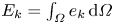 $E_k= \int _{\varOmega } e_k \, {\rm d}\varOmega$) can be obtained
 \begin{equation} \frac{\partial E_k}{\partial t} = E_{s} + E_{b} + E_{v}, \end{equation}
where
 \begin{equation} \left.\begin{gathered} E_{s}= Re \left (- \int_{\varOmega} u_{p,j} \, \frac{\partial u_i}{\partial x_j} \, \bar{u}_{p,i} \, {\rm d}\varOmega \right ),\\ E_{b}= Re \left ( \frac{{\textit{Ra}}}{{\textit{Pr}}} \, \int_{\varOmega} T_p \, \bar{u}_{p,i} \delta_{i1} \, {\rm d}\varOmega \right ),\\ E_{v}= Re \left (- \int_{\varOmega} \frac{\partial u_{p,i}}{\partial x_j}\,\frac{\partial \bar{u}_{p,i}}{\partial x_j} \, {\rm d}\varOmega \right ). \end{gathered}\right\} \end{equation}
Since no acoustic force term appears in the perturbation equations, the rate of change of the total fluctuating kinetic energy has 3 contributions:  $E_{s}$ represents the production of fluctuating kinetic energy by shear of the basic flow (inertia term),
  $E_{b}$ the production of fluctuating kinetic energy by buoyancy and
  $E_{v}$ the viscous dissipation of fluctuating kinetic energy. At threshold, the critical eigenvector is associated with an eigenvalue with zero real part. This implies that
  ${\partial E_k / \partial t}$ is equal to zero at marginal stability. Finally, we normalize (2.4) by
  $-E_{v}=|E_{v}|$, which is always positive, to get an equation involving normalized energy terms
  $E'=E/|E_{v}|$ at threshold
 \begin{equation} E'_{s} + E'_{b} =1. \end{equation}
 Finally, the critical Rayleigh number can also be expressed as a function of energetic contributions. For that, we use the fact that the expression of  $E'_{b}$ linearly depends on
  ${\textit {Ra}}$. At the threshold, we can write
  $E'_{b} = {\textit {Ra}}_c E''_{b}$. And from (2.6), we get
  ${\textit {Ra}}_c E''_{b} = 1- E'_{s}$ which, for
  $A=0$, i.e. in the pure buoyancy case, gives
  ${\textit {Ra}}_0 E''_{b,0} = 1$, where the subscript 0 refers to the case
  $A=0$ and
  ${\textit {Ra}}_0={\textit {Ra}}_c(A=0)$. Finally, the ratio of these two equations gives
 \begin{equation} \frac{{\textit{Ra}}_c}{{\textit{Ra}}_0} = \frac{ \overbrace{(1- E'_{s})}^{{R_{s}}}}{ \underbrace{ \left ( { E''_{b} / E''_{b_0} } \right ) }_{{R_{b}}} } , \end{equation}
which indicates that the variation of  ${\textit {Ra}}_c$ with
  $A$ can be expressed through the ratio of the two quantities
  $R_{s}$ and
  $R_{b}$, the first quantity being connected to the shear of the basic flow due to acoustic streaming and the second quantity to buoyancy. For
  $A=0$,
  $R_{s}$ and
  $R_{b}$ are equal to 1 and
  ${\textit {Ra}}_c={\textit {Ra}}_0$.
3. Numerical methods and tests of accuracy
The 2-D steady calculations were performed with the 2-D version of the spectral element code with continuation techniques developed by Henry & Ben Hadid (Reference Henry and Ben Hadid2007), further used by Torres et al. (Reference Torres, Henry, Komiya, Maruyama and Ben Hadid2013, Reference Torres, Henry, Komiya and Maruyama2014) and more recently adapted to non-Newtonian fluids by Henry et al. (Reference Henry, Millet, Dagois-Bohy, Botton and Ben Hadid2022). In this code, Newton–Krylov methods are used to compute both the steady flow solutions taking into account the acoustic streaming force and the bifurcation points at which these solutions are destabilized by steady or oscillatory perturbations.
For transient computations or unsteady flow simulations, an accurate time stepping of the equations discretized on the spectral element mesh is performed using the third-order accurate time integration scheme proposed by Karniadakis, Israeli & Orszag (Reference Karniadakis, Israeli and Orszag1991). Finally, for the specific calculation of periodic orbits (or cycles), we used the cycle continuation method developed by Medelfef et al. (Reference Medelfef, Henry, Bouabdallah and Kaddeche2019), but originally proposed by Sánchez et al. (Reference Sánchez, Net, García-Archilla and Simó2004) and already successfully used in a Rayleigh–Bénard problem by Puigjaner et al. (Reference Puigjaner, Herrero, Simó and Giralt2011). The method is still based on a Newton–Krylov approach in which the periodic states of (2.1)–(2.3) are obtained as fixed points of a Poincaré map. The trajectories in the phase space used to approach the periodic state are computed with the time integration scheme at second or third order with a small time step  $\Delta t$. The method is found to work well with a convergence generally obtained with a few Newton–Krylov steps (3 to 7), each Newton–Krylov step requiring 1 to 4 generalized minimal residual algorithm (GMRES) iterations for a prescribed precision of
  $10^{-2}$. The stability of these periodic solutions is further investigated in the framework of the Floquet theory using an Arnoldi method (Medelfef et al. Reference Medelfef, Henry, Bouabdallah and Kaddeche2019). In our previous work (Medelfef et al. Reference Medelfef, Henry, Bouabdallah and Kaddeche2019), a time integration scheme at third order was always used. Here, for some cases, the period is so long that the time step has to be increased and this is only possible with a scheme at second order. In order to be sure that the corresponding loss of accuracy was acceptable, we performed some tests on the calculation of the periodic solution at
  $A=4000$ and
  ${\textit {Ra}}=6760$, a case for which both schemes and different time steps can be used. For the different tests, the period and the two first Floquet multipliers related to the calculated cycle are given in table 1. We see that, for a time step
  $\Delta t= 10^{-5}$, the schemes at order 2 and 3 give practically the same results, with differences only affecting the seventh digit for the period and the sixth digit for the Floquet multipliers. The scheme at order 2 with
  $\Delta t= 10^{-4}$ yields results which are also very close. Even the scheme at order 2 with
  $\Delta t= 10^{-3}$ provides acceptable results, with a relative error on the period of
  $5 \times 10^{-4}$ with respect to the reference case at order 3.
Table 1. Periodic oscillatory solution obtained at  $A=4000$ and
  ${\textit {Ra}}=6760$ with different time schemes and time steps (for
  $A=4000$, the oscillatory instability threshold is at
  ${\textit {Ra}}_c=6609.92$). We compare the period of the computed oscillatory solution and the first two Floquet multipliers Floq
 $_1$ and Floq
 $_2$ (those with the strongest norm) obtained by the Arnoldi method, which are real in this case (2-D cavity with
  $A_y=10$,
  $H_b=0.338$,
  $ {\textit {Pr}}=1$).

The grid used for all our calculations of streaming flow in a Rayleigh–Bénard cavity with an aspect ratio  $A_y=10$ has
  $N_y=101 \times N_x=87$ points in the
  $y$ and
  $x$ directions, respectively. The number of points
  $N_x$ in the short vertical
  $x$ direction is higher than needed: this choice comes from our previous study (Ben Hadid et al. Reference Ben Hadid, Dridi, Botton, Moudjed and Henry2012), where we wanted to very progressively vary the beam width. Tests have been done to check the quality of the discretization along the horizontal
  $y$ direction. As shown in table 2, where the number of points
  $N_y$ in the
  $y$ direction is varied, the chosen grid gives an excellent resolution of the problem. The thresholds at different bifurcation points do not evolve or only very little when
  $N_y$ is increased. The very good tests on the Hopf thresholds indicate that both the flow solution and the eigenvector that will induce the oscillatory behaviour are well resolved on the grid. The tests on the saddle-node points at which steady solutions appear are also excellent.
Table 2. Tests of accuracy for the simulations. The critical values at different primary Hopf bifurcation points (see figure 8) and saddle nodes (SN) points (on the upper solid black curve  $SN_{U_2}$ in figure 20) are given for different numbers of grid points in the horizontal
  $y$ direction. The number of grid points
  $N_x$ in the vertical
  $x$ direction is kept at 87, a sufficiently high value (2-D cavity with
  $A_y=10$,
  $H_b=0.338$,
  $ {\textit {Pr}}=1$).

4. Streaming flows without buoyancy ( ${\textit {Ra}}=0$)

In the absence of buoyancy ( ${\textit {Ra}}=0$), steady numerical solutions of the system (2.1)–(2.3) in a 2-D cavity of aspect ratio
  $A_y=10$ have been obtained for a beam width
  $H_b=0.338$, a Prandtl number
  $ {\textit {Pr}}=1$ and different values of the acoustic streaming parameter
  $A$. The global view of the flow is shown in figure 2 through velocity vector plots. We see the typical stationary streaming structure of the Eckart flow in a bounded cavity: around the sound beam axis, the flow is directed away from the sound source, in the same direction as the acoustic waves propagation, whereas along the upper and lower walls, the flow is in the opposite direction, back to the source, allowing mass conservation in the closed cavity. The horizontal velocity profiles at mid-length in the cavity are plotted in figure 3 for different values of
  $A$. These profiles reproduce the positive
  $v$ values around the sound beam axis at
  $x=0$ and the negative
  $v$ values associated with the back flow along the upper and lower walls. These profiles are compared with the analytical parallel flow profiles obtained in an extended cavity (black
  $+$ symbols) and derived in Ben Hadid et al. (Reference Ben Hadid, Dridi, Botton, Moudjed and Henry2012). For all the values of
  $A$, the comparison is excellent, indicating that the parallel flow approximation is still valid in the central part of a cavity of aspect ratio
  $A_y=10$. Moreover, the direct proportionality of the velocity profiles with
  $A$ obtained analytically also applies to our numerical profiles and the changes of curvature in the profiles occur in any case at the limits of the beam. Finally, as expected for rather small beam widths, the region with positive velocities is larger than the beam width
  $H_b$ (only slightly here) and the maximum velocity occurs along the beam axis.
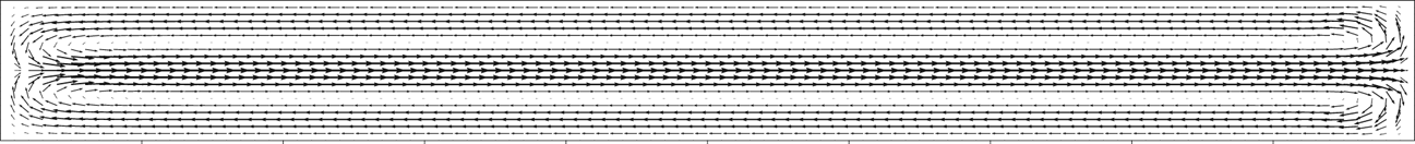
Figure 2. Characteristic streaming flow in the cavity with aspect ratio  $A_y=10$ for a beam width
  $H_b=0.338$ (
 ${\textit {Ra}}=0, A=2000, {\textit {Pr}}=1$).

Figure 3. Horizontal velocity profiles, characteristic of the streaming, at mid-length in the cavity with aspect ratio  $A_y=10$ for a beam width
  $H_b=0.338$ and different values of
  $A$ (1000, 2000, 3000, 4000, 5000, 6000, 6500,
  $A_c=7051.36$) (
 $ {\textit {Pr}}=1$). The profiles obtained for
  ${\textit {Ra}}=0$ (coloured lines, pure streaming) are compared with those obtained at the thresholds
  ${\textit {Ra}}_c$ (thick black dashed lines) and with the analytical parallel flow profiles in an extended cavity (black
  $+$ symbols, Ben Hadid et al. Reference Ben Hadid, Dridi, Botton, Moudjed and Henry2012). The horizontal dashed lines indicate the limits of the acoustic beam.
In our 2-D simulations, the flow must change direction at the endwalls through vertical  $u$ velocities, which are plotted for
  $A=4000$ in figure 4(a,b) (solid isocontours) with zooms on the two extremities of the cavity. These vertical velocities have their larger values in the end parts, principally on a length of approximately
  $1$, i.e. the height of the cavity. Outside these end parts, where the return of the flow occurs, the vertical velocities are rather small, in any case below 10 % of
  $u_{max}$ and 2 % of
  $v_{max}$ (maximum vertical and horizontal velocities in the cavity, respectively), and they still strongly decrease when moving towards the cavity centre. In this long central zone, the parallel flow approximation can then be considered as well verified. The isotherms for the same case (
 $A=4000$) are also given in figure 4(c,d) (solid isocontours). The heat transfer appears to be diffusive in the main part of the cavity, except in the same end parts where it is influenced by the vertical velocities. Note that these pure streaming steady flows have the up–down symmetry.

Figure 4. Vertical velocity (a,b) and isotherm (c,d) contours plots in the cavity for  $A=4000$ at the threshold
  ${\textit {Ra}}_c$ (dashed lines, see text in § 5 and table 3 for details) and at
  ${\textit {Ra}}=0$ (solid lines, pure streaming). Zooms on the end parts of the cavity (2-D cavity with
  $A_y=10$,
  $H_b=0.338$,
  $ {\textit {Pr}}=1$).
When the acoustic streaming parameter  $A$ is increased, the streaming flow is eventually destabilized by a Hopf bifurcation. Such thresholds for the pure streaming flow in a 2-D cavity (
 $A_y=10$) were already calculated by Ben Hadid et al. (Reference Ben Hadid, Dridi, Botton, Moudjed and Henry2012) for different beam widths
  $H_b$ and they were compared with the thresholds in an extended cavity (parallel flow approximation) obtained previously by Dridi et al. (Reference Dridi, Henry and Ben Hadid2010). For the 2-D situation studied here with
  $H_b=0.338$, the critical threshold is
  $A_c=7051.36$ and it corresponds to the minimum of the critical curve given in Ben Hadid et al. (Reference Ben Hadid, Dridi, Botton, Moudjed and Henry2012), i.e. to the more unstable situation. In an extended cavity, the thresholds are rather smaller, and the minimum threshold is obtained for
  $H_b\approx 0.32$ with
  $A_c=5143$ (Dridi et al. Reference Dridi, Henry and Ben Hadid2010).
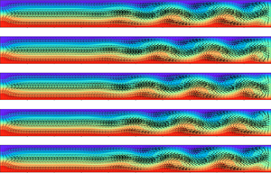
The perturbation at the Hopf bifurcation for  $A=A_c$ in our 2-D situation is shown in figure 5(i) through the vertical velocity isocontours of the critical eigenvector (real part). We see that the perturbation is concentrated near the right boundary of the cavity and has a arrowhead shape. Such perturbation will break the up–down symmetry of the pure streaming flow. It is associated with a critical angular frequency
  $\omega _c=16.8935$ and corresponds to a wave travelling towards the source, in the direction opposite to the beam propagation direction. Such waves will be denoted as backward waves, whereas those travelling in the beam propagation direction will be denoted as forward waves. This wave appears at a supercritical bifurcation, as shown by the regularly increasing cycle amplitude above the instability threshold in the phase diagram in figure 6. Its backward propagation is illustrated in figure 7 for
  $A=7200$ and
  ${\textit {Ra}}=0$ by the plots of the vertical velocity contours at different times during the period. Note that the wave, which is well represented by the vertical velocity, is mainly visible near the right boundary of the cavity, where it is initiated successively from the upper and lower recirculation zones.

Figure 5. Vertical velocity contour plots for the real part of the eigenvectors at the critical Rayleigh number  ${\textit {Ra}}_c$ for increasing values of the acoustic streaming parameter
  $A$ from 0 (Rayleigh–Bénard threshold,
  ${\textit {Ra}}_c={\textit {Ra}}_0=1728.83$) to
  $A_c=7051.36$ (pure streaming threshold at
  ${\textit {Ra}}=0$) through
  $A=1000$, 2000, 3000, 4000, 5000, 6000, 6500. The values of
  ${\textit {Ra}}_c$ are given in each case. The type of instability and the values of the critical angular frequency
  $\omega _c$ can be found in table 3 (2-D cavity with
  $A_y=10$,
  $H_b=0.338$,
  $ {\textit {Pr}}=1$).

Figure 6. Phase diagram giving the periodic orbits for values of  $A$ (
$A$ ( $7060, 7100, 7200, 7500$) close above the oscillatory instability threshold (
 $A_c=7051.36$, red open circle) for a pure streaming flow (
 ${\textit {Ra}}=0$, 2-D cavity with
  $A_y=10$,
  $H_b=0.338$,
  $ {\textit {Pr}}=1$). Here,
  $u_1$ and
  $u_2$ are the vertical velocities at the points (
 $x=0.16055, y=0$) and (
 $x=0.05437, y=0.46822$), respectively. The cycle presented in figure 7 is given in red.

Figure 7. Vertical velocity contour plots during a cycle at  $A=7200$ for a pure streaming flow (
 ${\textit {Ra}}=0$). The oscillatory instability threshold is at
  $A_c=7051.36$ and corresponds to the instability
  $I_4$ (see table 3). The period of this cycle is
  $T_{osc}=0.36812$ and 5 plots are given, each
  $T_{osc}/4$ from 0 to
  $T_{osc}$ (2-D cavity with
  $A_y=10$,
  $H_b=0.338$,
  $ {\textit {Pr}}=1$).
5. Buoyant instability thresholds in presence of streaming flows
When buoyancy is considered (here in a fluid with  $ {\textit {Pr}}=1$), the steady flow in the cavity heated from below will become unstable beyond a critical threshold expressed by the critical Rayleigh number
  ${\textit {Ra}}_c$. Without streaming (
 $A=0$), the steady flow is a pure diffusive temperature field (perfectly horizontal isotherms throughout the cavity), which has both the up–down and left–right symmetries, and the instability is steady and occurs at the critical threshold
  ${\textit {Ra}}_c=1728.83$, a value slightly larger than the well-known Rayleigh–Bénard value in an extended layer, due to the slight lateral confinement in our cavity with
  $A_y=10$. The critical eigenvector, shown through the vertical velocity in figure 5(a), corresponds to 10 counter-rotating rolls inside the cavity. It breaks the up–down symmetry, but keeps the left–right symmetry of the basic steady flow at threshold.
When the acoustic force is applied ( $A \neq 0$), the steady flow is modified by the presence of streaming and the instability generally becomes oscillatory beyond a modified threshold. The basic steady flow at threshold is close to the streaming flows presented in the previous section. However, as the thresholds generally occur at
  ${\textit {Ra}} \neq 0$ and the isotherms are slightly deformed by the streaming flow in the end parts, some buoyant flow will appear in these zones. To quantify this effect, the velocity profiles at mid-length in the cavity at the thresholds have also been plotted in figure 3 as thick black dashed lines. We see almost no effect on these profiles for all the values of
  $A$. We have also plotted the isocontours of vertical velocity and temperature in the end parts at the threshold in figure 4. The isocontours are given for
  $A=4000$, a value for which the threshold is quite high (
 ${\textit {Ra}}_c=6609.92$), and they appear as dashed lines. Compared with what is obtained at
  ${\textit {Ra}}=0$, the influence is perceptible in both the vertical velocity and temperature, but remains weak. Note that the basic flow at threshold keeps the up–down symmetry mentioned previously for the pure streaming flows at
  ${\textit {Ra}}=0$ in § 4.
The variation of the critical thresholds  ${\textit {Ra}}_c$ with the acoustic streaming parameter
  $A$ is given in figure 8. The thresholds first increase with
  $A$ from the value
  ${\textit {Ra}}_0=1728.83$ at
  $A=0$ to a maximum value close to
  $7346$ obtained for
  $A \approx 4800$. They decrease then quite rapidly to reach the pure streaming threshold (
 ${\textit {Ra}}=0$) at
  $A_c=7051.36$. Contrary to the case of the extended layer where a single critical curve was found from the buoyant threshold to the pure streaming threshold (Ben Hadid et al. Reference Ben Hadid, Dridi, Botton, Moudjed and Henry2012), the thresholds correspond here to four successive critical curves corresponding to four different instabilities denoted as
  $I_1$ to
  $I_4$. The corresponding eigenvectors which are presented in figure 5 change with the change of instability, but rather evolve with
  $A$ from the usual roughly circular Rayleigh–Bénard rolls occupying the whole cavity to deformed rolls concentrated in the right end part.

Figure 8. Critical curves for the onset of instability in the Rayleigh–Bénard–Eckart problem in a long 2-D cavity, expressed as  ${\textit {Ra}}_c$ as a function of
  $A$ (
$A$ ( $A_y=10, H_b=0.338, {\textit {Pr}}=1$). Four different instabilities (from
  $I_1$ to
  $I_4$) determine the critical curve from the pure Rayleigh–Bénard threshold at
  ${\textit {Ra}}_0=1728.83$ to the pure streaming threshold at
  $A_c=7051.36$.
The variation of the critical angular frequency at threshold,  $\omega _c$, with the acoustic streaming parameter
  $A$ is given in figure 9. The angular frequency (which is zero for
  $A=0$, steady threshold) appears to be negative for the small values of
  $A$ and to change sign and become positive above a value of
  $A$ between 1900 and 2000. The change of critical instability also induces jumps in the variation of
  $\omega _c$.

Figure 9. Critical angular frequency at the onset of instability in the Rayleigh–Bénard–Eckart problem in a long 2-D cavity expressed as  $\omega _c$ as a function of
  $A$ (
$A$ ( $A_y=10, H_b=0.338, {\textit {Pr}}=1$).
In fact, these instabilities occur at Hopf bifurcation points with complex conjugate eigenvectors, associated with  $\pm \omega _c$. The sign of
  $\omega _c$ plotted in figure 9 is then not enough to determine the phase speed of the perturbations (corresponding to waves) and the consideration of the real and imaginary parts of the critical eigenvectors is needed. If
  $H$ is the complex eigenvector associated with the angular frequency
  $\omega$, which has a sign
  $s_{\omega }$, the time evolution of the perturbation will be given by
 \begin{align} {\rm Re} \left[H \exp({\rm i} \omega t)\right]={\rm Re} \left[(H_r + {\rm i} H_i) (\cos(\omega t) + {\rm i} \sin(\omega t))\right] = H_r \cos(\omega t) - H_i \sin(\omega t), \end{align}
where  $\textrm {Re}$ denotes the real part, i is the unit imaginary number and
  $H_r$ and
  $H_i$ refer to the real and imaginary parts of the eigenvector, respectively. To find the propagation direction of the waves, we can consider the evolution of the perturbations at different successive times during a period
  $T_{osc}=2 {\rm \pi}/\omega$, for example at
  $t=0$,
  $t=T_{osc}/4$,
  $t=T_{osc}/2$,
  $t=3 T_{osc} /4$. Using (5.1), we obtain the corresponding perturbations at those times, which are
  $H_r$,
  $-H_i s_{\omega }$,
  $-H_r$,
  $H_i s_{\omega }$, respectively. In figure 10, as an example, we give the vertical velocity isocontours for the real and imaginary parts of the eigenvector at
  $A=4000$, which are associated with the critical threshold and angular frequency given in figures 8 and 9, respectively. For this case at
  $A=4000$,
  $\omega _c$ is positive (figure 9), so that the time evolution of the perturbation during a period will correspond to
  $H_r$,
  $-H_i$,
  $-H_r$,
  $H_i$. In practice, for example, the red zone (associated with positive vertical velocities) close to the right wall in
  $H_r$ (corresponding to
  $t=0$) is found to evolve towards the left in successively
  $-H_i$ at
  $t=T_{osc}/4$ (the main blue zone in
  $H_i$ which becomes red in
  $-H_i$),
  $-H_r$ at
  $t=T_{osc}/2$ (the main blue zone in
  $H_r$ which becomes red in
  $-H_r$) and finally
  $H_i$ at
  $t=3 T_{osc} /4$ (the second red zone from the right in
  $H_i$) (figure 10). This indicates that the positive values of
  $\omega _c$ obtained for the large values of
  $A$ in figure 9 correspond to left travelling waves (backward waves) and the negative values obtained for small
  $A$ to right travelling waves (forward waves). In our situation, we then obtain forward waves at small
  $A$, close to the Rayleigh–Bénard threshold, and backward waves for larger
  $A$, as in the pure streaming case (
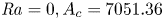 ${\textit {Ra}}=0, A_c=7051.36$).

Figure 10. Vertical velocity contour plots of the eigenvectors associated with a positive angular frequency  $\omega _c$ at
  ${\textit {Ra}}_c$ for
  $A=4000$ (see figure 9). The first plot (a) corresponds to the real part and the second plot (b) to the imaginary part of the eigenvector (2-D cavity with
  $A_y=10$,
  $H_b=0.338$,
  $ {\textit {Pr}}=1$).
To depict the origin of the instabilities, the variations with  $A$ of the different contributions to the total kinetic energy budget at threshold (2.6) are shown in figure 11(a). We see that both buoyancy and shear contributions are destabilizing (positive values) and they together balance the stabilizing dissipation (negative values). The normalized shear contribution
  $E'_s$ increases from 0 at
  $A=0$ to 1 at
  $A=A_c$, while the normalized buoyancy contribution
  $E'_b$ decreases from 1 to 0, and the change of critical eigenvector from
  $I_1$ to
  $I_4$ does not affect much these variations. This indicates that the instability evolves regularly from buoyancy induced at
  $A=0$ to shear induced at
  $A=A_c$.

Figure 11. Contributions to the total fluctuating kinetic energy budget ( $E'_s$ (shear, solid curve),
  $E'_b$ (buoyancy, dashed curve)) (a) and energy factors
  $R_s$ (connected to shear, solid curve) and
  $R_b$ (connected to buoyancy, dashed curve) (b) for the critical perturbations at threshold as a function of the acoustic streaming parameter
  $A$ (2-D cavity with
  $A_y=10$,
  $H_b=0.338$,
  $ {\textit {Pr}}=1$).
As shown in § 2, the critical Rayleigh number can also be expressed as a function of energetic contributions,  $R_{s}$ connected to shear and
  $R_b$ connected to buoyancy (
 ${\textit {Ra}}_c/{\textit {Ra}}_0=R_{s}/R_b$, (2.7)). The variations with
  $A$ of these two quantities
  $R_{s}$ and
  $R_b$ are shown in figure 11(b);
  $R_{s}$ and
  $R_b$ continuously decrease as
  $A$ is increased, but
  $R_{s}$ decreases from 1 for
  $A=0$ to 0 for
  $A=A_c$ whereas
  $R_b$ decreases from 1 to approximately 0.015, a small but non-zero limiting value. Moreover, the initial decrease of
  $R_{s}$ is small, corresponding to a small initial shear destabilization
  $E'_s$, whereas the initial decrease of
  $R_b$ is strong, corresponding to a strong decrease of the destabilizing buoyancy contribution
  $E''_b$. These initial variations leading to
  $R_{s} \gg R_b$ explain the initial increase of
  ${\textit {Ra}}_c$, i.e. the stabilizing effect. For larger
  $A$, the curve of
  $R_s$ gets the stronger decrease, which limits the increase of
  ${\textit {Ra}}_c$ and induces its further decrease. Finally, the curves of
  $R_{s}$ and
  $R_b$ eventually cross (which corresponds to
  ${\textit {Ra}}_c={\textit {Ra}}_0$), which allows the ultimate decrease of
  ${\textit {Ra}}_c$ toward 0 for
  $A=A_c$.
These energy analyses confirm those obtained in an extended layer (Ben Hadid et al. Reference Ben Hadid, Dridi, Botton, Moudjed and Henry2012). As in this previous study, the variation of the instability thresholds when streaming is applied is strongly connected with the changes of the perturbation fields that occur when  $A$ is increased.
6. Characteristics of the flows triggered at the instability thresholds
The real perturbation at the pure Rayleigh–Bénard threshold ( $A=0$) generates a steady flow, which breaks the up–down symmetry of the diffusive basic state. Two stable solutions, related by the broken symmetry, then appear at this pitchfork bifurcation. One of these solutions is shown in figure 12 through the velocity field for
  ${\textit {Ra}}=3000$. We see that these steady solutions correspond to 10 counter-rotating regular rolls inside the cavity and that they keep the left–right symmetry of the basic state.

Figure 12. Velocity vectors plot for the steady flow in the pure Rayleigh–Bénard situation ( $A=0$) at
  ${\textit {Ra}}=3000$. The steady threshold is at
  ${\textit {Ra}}_c=1728.83$ (2-D cavity with
  $A_y=10$,
  $H_b=0.338$,
  $ {\textit {Pr}}=1$).
When streaming becomes effective ( $A \neq 0$), the perturbations at the Hopf thresholds are expected to generate oscillatory flows. These flows have been found to be time periodic, at least close to the thresholds, and to belong to supercritical branches. To obtain these periodic flows, we have used the cycle continuation method presented in § 3 and more precisely described in Medelfef et al. (Reference Medelfef, Henry, Bouabdallah and Kaddeche2019).
The periodic flows have first been calculated in a certain range of Rayleigh number beyond the critical threshold  ${\textit {Ra}}_c$ for different values of the acoustic streaming parameter
  $A$, up to the pure streaming threshold at
  $A_c=7051.36$ (
 $A=1000, 2000, 3000, 4000, 5000, 6000, 6500, A_c$). For these values of
  $A$, the critical characteristics at the oscillatory transition are given in table 3. To characterize the dynamics of these periodic orbits in the phase space, we have chosen to generally follow two velocities
  $u_1$ and
  $u_2$, which are the vertical velocities at the points (
 $x=0.16055, y=0$) and (
 $x=0.05437, y=0.46822$), respectively. In the following, we present the characteristics of the periodic orbits appearing above the thresholds for the different instabilities
  $I_1$ to
  $I_4$ for selected values of
  $A$.
$A$.
Table 3. Critical characteristics, type of instability, Rayleigh number  ${\textit {Ra}}_c$, angular frequency
  $\omega _c$ and period
  $T_{osc,c}$ at the instability thresholds for different values of the acoustic streaming parameter
  $A$ from 0 (Rayleigh–Bénard threshold) to
  $A_c$ (pure streaming threshold) (2-D cavity with
  $A_y=10$,
  $H_b=0.338$,
  $ {\textit {Pr}}=1$).
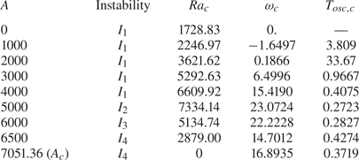
6.1. Forward waves for the instability $I_1$ at $A=1000$


In our 2-D cavity, for small values of  $A$, the steady perturbation of the Rayleigh–Bénard situation (
 $A=0$) will become oscillatory and progress away from the transducer, in the direction of the beam propagation, giving what we have called a forward wave. Such forward wave is illustrated in figure 13 for
  $A=1000$ and
  ${\textit {Ra}}=2400$ by the plots of the vertical velocity contours at different times during the period. The perturbation, initiated at the left endwall, is still not much deformed by the streaming flow. It is more intense in the right half of the cavity, but remains visible in the whole cavity. The bifurcation diagram and phase diagram for
  $A=1000$ are also given in figure 14. We see that the bifurcation is supercritical and that the cycle amplitude at
  $u_1$ increases with
  ${\textit {Ra}}$ above the threshold. The period, which is
  $T_{osc,c}=3.809$ at threshold, first decreases down to approximately
  $3.68$ at
  ${\textit {Ra}}=2450$ and then increases (see figure 15).

Figure 13. Vertical velocity contour plots during a cycle at  $A=1000$ and for
  ${\textit {Ra}}=2400$ (the oscillatory instability threshold is at
  ${\textit {Ra}}_c=2246.97$ and corresponds to the instability
  $I_1$, see table 3). The period of this cycle is
  $T_{osc}=3.6790$ and 5 plots are given, each
  $T_{osc}/4$ from 0 to
  $T_{osc}$ (2-D cavity with
  $A_y=10$,
  $H_b=0.338$,
  $ {\textit {Pr}}=1$).

Figure 14. Bifurcation diagram (a) and phase diagram (b) giving the periodic orbits above the oscillatory instability threshold ( ${\textit {Ra}}_c=2246.97$, red open circle) for
  $A=1000$ in a 2-D cavity with aspect ratio
  $A_y=10$ (
 $H_b=0.338$,
  $ {\textit {Pr}}=1$). The cycle presented in figure 13 is given in red.

Figure 15. Variation of the period beyond the oscillatory instability threshold (given as a red open circle) for different values of the acoustic streaming parameter  $A$. The characteristics at the critical thresholds, type of instability, critical Rayleigh number
  ${\textit {Ra}}_c$ and critical period
  $T_{osc,c}$ are given in table 3 (2-D cavity with
  $A_y=10$,
  $H_b=0.338$,
  $ {\textit {Pr}}=1$).
6.2. Backward waves for the instability $I_1$ at $A=4000$


For larger values of  $A$ (
$A$ ( $A \geq 2000$), backward waves, i.e. waves travelling in the direction opposite to the beam propagation, are expected. Such backward wave is illustrated in figure 16 for
  $A=4000$ and
  ${\textit {Ra}}=6800$ by the plots of the velocity vectors fields at different times during the period. This case is on the same branch of instability (instability
  $I_1$) as the previous case at
  $A=1000$, but the instability has evolved with the stronger influence of the streaming on both its shape and its localization in the cavity (figure 5e). For
  ${\textit {Ra}}=6800$, i.e. not far from the oscillatory instability threshold at
  ${\textit {Ra}}_c=6609.92$, the instability has already well developed, giving a wavy shape to the streaming jet, with eddies alternately arranged on its both sides. The isotherms, given in figure 16(e), are also well deformed, with a wavy shape following that of the jet. The bifurcation diagram and phase diagram for
  $A=4000$ are given in figure 17. Here also, the bifurcation is supercritical and the cycle amplitude at
  $u_1$ increases with
  ${\textit {Ra}}$ above the threshold, very slowly close to the threshold, quickly around
  $A=6800$, and then more slowly beyond
  $A=7100$. The period, which is
  $T_{osc,c}=0.4075$ at threshold, regularly increases, reaching the value
  $0.5806$ at
  ${\textit {Ra}}=7600$ and
  $0.7862$ at
  ${\textit {Ra}}=8540.7$ (figure 15).

Figure 16. Velocity vectors plots during a cycle at  $A=4000$ and for
  ${\textit {Ra}}=6800$ (the oscillatory instability threshold is at
  ${\textit {Ra}}_c=6609.92$ and corresponds to the instability
  $I_1$, see table 3). The period of this cycle is
  $T_{osc}=0.4419$ and 5 plots are given, each
  $T_{osc}/4$ from 0 to
  $T_{osc}$. For
  $t=T_{osc}$ (last plot e), the isotherms are also given (2-D cavity with
  $A_y=10$,
  $H_b=0.338$,
  $ {\textit {Pr}}=1$).

Figure 17. Bifurcation diagram (a) and phase diagram (b) giving the periodic orbits above the oscillatory instability threshold ( ${\textit {Ra}}_c=6609.92$, red open circle) for
  $A=4000$ in a 2-D cavity with aspect ratio
  $A_y=10$ (
 $H_b=0.338, {\textit {Pr}}=1$). The cycle presented in figure 16 is given in red.
6.3. Backward waves for the other instabilities $I_2$, $I_3$ and $I_4$


We have seen that the critical curve (figure 8) involves other instabilities than  $I_1$ when the acoustic streaming parameter
  $A$ is increased. The waves connected with the instability
  $I_4$ have been illustrated in figure 7 for
  $A=A_c$. We now show the waves corresponding to the instability
  $I_2$ for
  $A=5000$ and
  ${\textit {Ra}}=7500$ and the instability
  $I_3$ for
  $A=6000$ and
  ${\textit {Ra}}=5400$ in figures 18 and 19, respectively. For these two instabilities, the waves are backward waves, which look similar to those obtained for the instability
  $I_4$ at
  $A=A_c$, with an even stronger localization near the right endwall. The velocity vectors plots used to depict the waves for
  $A=6000$ show that, for
  ${\textit {Ra}}=5400$, the perturbation of the streaming jet remains moderate and is only visible through a slight undulation of the jet close to the right endwall. Comparing these results with those shown in figure 16, we thus observe a strong variation between the waves of the instability
  $I_1$ at
  $A=4000$ and those of the instability
  $I_2$ at
  $A=5000$ and the instability
  $I_3$ at
  $A=6000$. Concerning the period of these cycles, for the three instabilities
  $I_2$,
  $I_3$ and
  $I_4$, the periods are rather short (
 $T_{osc}<0.5$). They regularly increase above the thresholds when
  ${\textit {Ra}}$ is increased, but in a rather moderate way (figure 15).

Figure 18. Vertical velocity contour plots during a cycle at  $A=5000$ and for
  ${\textit {Ra}}=7500$ (the oscillatory instability threshold is at
  ${\textit {Ra}}_c=7334.14$ and corresponds to the instability
  $I_2$, see table 3). The period of this cycle is
  $T_{osc}=0.27645$ and 5 plots are given, each
  $T_{osc}/4$ from 0 to
  $T_{osc}$ (2-D cavity with
  $A_y=10$,
  $H_b=0.338$,
  $ {\textit {Pr}}=1$).

Figure 19. Velocity vectors plots during a cycle at  $A=6000$ and for
  ${\textit {Ra}}=5400$ (the oscillatory instability threshold is at
  ${\textit {Ra}}_c=5134.74$ and corresponds to the instability
  $I_3$, see table 3). The period of this cycle is
  $T_{osc}=0.28639$ and 5 plots are given, each
  $T_{osc}/4$ from 0 to
  $T_{osc}$ (2-D cavity with
  $A_y=10$,
  $H_b=0.338$,
  $ {\textit {Pr}}=1$).
7. More global dynamics showing the competition between waves and steady solutions
The periodic orbits shown in the previous section, which correspond to forward waves at small values of  $A$ and backward waves at larger
  $A$ up to
  $A_c$, belong in fact to limited regions in the
  $({\textit {Ra}},A)$ parameter space. This is shown in figure 20, in the global stability diagram which has been uncovered by a detailed study. We see that the forward and backward waves (denoted FW and BW, respectively, in the plot) belong to regions delimited by the Hopf thresholds and by saddle-node curves which are initiated close to
  $A=2000$, in the region of sign change for
  $\omega _c$. To describe the complex stability diagram in figure 20 and the global dynamics it involves, we will then first focus on what occurs close to the change of sign of
  $\omega _c$ and particularly for
  $A=2000$.

Figure 20. Stability diagram giving the critical Rayleigh number  ${\textit {Ra}}_c$ for the oscillatory instability threshold (black dashed line) and the steady thresholds (solid lines) in large ranges of the acoustic streaming parameter
  $A$ and the Rayleigh number
  ${\textit {Ra}}$ (2-D cavity with
  $A_y=10$,
  $H_b=0.338$,
  $ {\textit {Pr}}=1$). The steady thresholds given by the black solid curves
  $SN_L$,
  $SN_{U_1}$ and
  $SN_{U_2}$ correspond to saddle-node points which delimit domains of existence of stable steady solutions. The coloured curves refer to the saddle-node points mentioned in figure 29.
  $P_{SN}$ is the limit point of the saddle-node curves
  $SN_{U_1}$ and
  $SN_{U_2}$. Here, FW and BW indicate the domains of forward and backward waves, respectively, which are delimited by the Hopf curve and saddle-node curves. A zoom of what occurs at the sign change for
  $\omega _c$ (close to
  $A=2000$) is given in figure 28.
7.1. Specific dynamics for $A=2000$

The bifurcation diagram for  $A=2000$ and its associated phase diagram are presented in figure 21. For
  $A=2000$, it is possible to obtain the backward wave predicted at the threshold
  ${\textit {Ra}}_c=3621.62$ only in a small
  ${\textit {Ra}}$ range above the threshold and then with a weak amplitude (cycles coloured in blue in figure 21). Such a backward wave is presented in figure 22 at different times during the period for
  ${\textit {Ra}}=3630$. The wave has a weak intensity and a long period. In contrast with the previous cases, its travel inside the cavity does not seem regular during the period (figure 22). Moreover, the calculated period at
  ${\textit {Ra}}=3630$ is
  $T_{osc}=41.711$, a value already much stronger than the critical value at the very close threshold,
  $T_{osc,c}=33.67$. Such cycles are obtained up to
  ${\textit {Ra}}=3640$, but not for
  ${\textit {Ra}}=3650$ where steady solutions are finally reached. Following these steady solutions by continuation, it was found that they belong to a closed curve extending between saddle-node points at
  ${\textit {Ra}}_c=3642.27$ and
  ${\textit {Ra}}_c=3711.24$. Those steady solutions, however, are stable only along the upper and lower parts of the closed curve in figure 21(a), where we can find the blue solid circles corresponding to the two stable solutions at
  ${\textit {Ra}}=3650$. The steady flow corresponding to one of these stable solutions is given in figure 23 where we see the steady wavy shape of the jet, the other stable steady solution being obtained by up–down symmetry. Finally, for values of
  ${\textit {Ra}}$ above the steady solutions range (
 ${\textit {Ra}} \geq 3720$), it was again possible to get cycles (solid green curves in figure 21), but they now correspond to forward waves and appear with an already large amplitude, which then increases with
  ${\textit {Ra}}$. In fact, we observe a kind of continuity between the amplitude increase of the backward waves, the stable steady solutions and the forward waves. As an example of forward wave, we give the cycle obtained at
  ${\textit {Ra}}=3800$ in figure 24. This cycle is characterized by a rather moderate period
  $T_{osc}=15.233$ and a seemingly regular travel of the wave.

Figure 21. Bifurcation diagram (a) and phase diagram (b) giving the solutions above the oscillatory instability threshold ( ${\textit {Ra}}_c=3621.62$, red open circle) for
  $A=2000$ in a 2-D cavity with aspect ratio
  $A_y=10$ (
 $H_b=0.338, {\textit {Pr}}=1$). The cycles in blue correspond to backward waves, whereas those in green correspond to forward waves. Among these cycles, those presented in figures 22 and 24 are given in red. The dashed left green curve in (a) (inner green curve in (b)) corresponds to the cycle at
  ${\textit {Ra}}=3710$ and its evolution with time is shown in figure 25(b). The black arrows in (b) indicate the direction of the evolution along the cycles, clockwise and counterclockwise for the cycles associated with backward and forward waves, respectively. The steady solutions are found along the solid black curve, but they are stable only along the upper and lower parts of this curve in (a), where we can find the blue solid circles corresponding to
  ${\textit {Ra}}=3650$.

Figure 22. Vertical velocity contour plots during a cycle at  $A=2000$ and for
  ${\textit {Ra}}=3630$ (the oscillatory instability threshold is at
  ${\textit {Ra}}_c=3621.62$, see table 3). The period of this cycle is
  $T_{osc}=41.711$ and 5 plots are given, each
  $T_{osc}/4$ from 0 to
  $T_{osc}$ (2-D cavity with
  $A_y=10$,
  $H_b=0.338$,
  $ {\textit {Pr}}=1$).

Figure 23. Velocity vectors plot for the steady flow obtained for  $A=2000$ at
  ${\textit {Ra}}=3650$ (2-D cavity with
  $A_y=10$,
  $H_b=0.338$,
  $ {\textit {Pr}}=1$).

Figure 24. Vertical velocity contour plots during a cycle at  $A=2000$ and for
  ${\textit {Ra}}=3800$ (the oscillatory instability threshold is at
  ${\textit {Ra}}_c=3621.62$, see table 3). The period of this cycle is
  $T_{osc}=15.233$ and 5 plots are given, each
  $T_{osc}/4$ from 0 to
  $T_{osc}$ (2-D cavity with
  $A_y=10$,
  $H_b=0.338$,
  $ {\textit {Pr}}=1$).
Some interesting information can be obtained from the change of the cycles and their periods when  ${\textit {Ra}}$ is increased. For that, the time evolution of
  $u_1$ along a period for some of the cycles at
  $A=2000$ is shown in figure 25 and the variation of their period is given in table 4 and plotted in figure 26. When
  ${\textit {Ra}}$ is increased, we first see the strong increase of the period for the backward waves from the value at the threshold
  $T_{osc,c}=33.67$ to
  $T_{osc}=88.374$ at
  ${\textit {Ra}}=3640$. Beyond the steady solutions range, we then observe a strong decrease of the period for the forward waves, from
  $T_{osc}=56.538$ at
  ${\textit {Ra}} \approx 3718$ to the minimum
  $T_{osc} \approx 5.85$ at
  ${\textit {Ra}} \approx 4680$, before a further increase (figure 26). The shape of the cycles also strongly changes in the
  ${\textit {Ra}}$ range of increasing period for the backward waves and of decreasing period for the forward waves (figure 25). The cycles no longer have a classical temporal sine shape, but present alternatively time periods with strong evolution and time periods with weak evolution. The ultimate (asymptotic) shape at very large period can correspond to what is obtained at
  ${\textit {Ra}}=3710$ by time stepping, the period
  $T_{osc} \approx 864.9$ being too long to use the cycle continuation method in this case. The time evolution of
  $u_1$ for this case of forward wave is shown in figure 25(b) and its plot in the bifurcation and phase diagrams in figure 21 is given as dashed green curves. In figure 25(b), we see that the cycle remains a long time (
 $t \approx 400$) at an almost constant negative value of
  $u_1$, in the neighbourhood of the steady solutions with negative
  $u_1$ values (see figure 21), then evolves rapidly towards the opposite positive value of
  $u_1$, now in the neighbourhood of the other steady solutions with positive
  $u_1$ values, where it remains a long time, before returning rapidly close to the former steady solutions. Such an evolution is typical of a heteroclinic cycle. A similar, however, less marked, evolution can be found for the cycle associated with backward waves at
  ${\textit {Ra}}=3640$. As seen in figure 21, this cycle (right blue curve in (a) and outer blue curve in (b)) visits the neighbourhood of the steady solutions, which induces a longer time spent close to these steady solutions (figure 25a). We can then think that the cycles corresponding to backward waves (forward waves) will evolve towards long period heteroclinic cycles as they get closer to the steady solutions when
  ${\textit {Ra}}$ is increased (decreased). In both cases, the cycles are expected to disappear at heteroclinic bifurcations.

Figure 25. Time evolution of  $u_1$ for periodic solutions obtained at different values of
  ${\textit {Ra}}$ above the Hopf threshold (
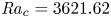 ${\textit {Ra}}_c=3621.62$) for
  $A=2000$ in a 2-D cavity with aspect ratio
  $A_y=10$ (
 $H_b=0.338$,
  $ {\textit {Pr}}=1$). In (a), the evolution is given during a period for the cycles at
  ${\textit {Ra}}=3630$ and 3640 corresponding to backward waves (blue solid curves) and the cycles at
  ${\textit {Ra}}=3720$, 3740 and 3800 corresponding to forward waves (green solid curves). In (b), the evolution corresponds to the very long period oscillatory solution obtained at
  ${\textit {Ra}}=3710$ (forward wave). The solution remains a long time close to the steady solutions with negative
  $u_1$ values, then evolves rapidly towards the other steady solutions with positive
  $u_1$ values where it remains for a long time, before returning rapidly close to the former steady solutions (see the cycle in the phase space in figure 21b).
Table 4. Period  $T_{osc}$ of the oscillatory solutions obtained at
  $A=2000$ for increasing values of
  ${\textit {Ra}}$ above
  ${\textit {Ra}}_c=3621.62$ for which the critical period is
  $T_{osc,c}=33.67$.


Figure 26. Variation of the period beyond the oscillatory instability thresholds (given as open circles) for two values of the acoustic streaming parameter,  $A=1000$ and 2000 (2-D cavity with
  $A_y=10$,
  $H_b=0.338$,
  $ {\textit {Pr}}=1$).
7.2. Dynamics in the neighbourhood of $\omega _c$ sign change

The study for  $A=2000$ has shown the existence of steady solutions in a certain
  ${\textit {Ra}}$ range, on a closed curve. The change of this curve when
  $A$ is decreased is shown in figure 27. For
  $A=1970$, the curve has evolved, but with a similar shape, and it appears in a lower
  ${\textit {Ra}}$ range. In contrast, for
  $A=1953.14$, there is a clear change of shape of the steady solutions curve, which accompanies the lowering of the
  ${\textit {Ra}}$ range. The change seems to be connected with the collision between two previous saddle-node points, which gives two new steady bifurcation points. If we now fix
  ${\textit {Ra}}$, the steady solutions also belong to a closed curve, which is now limited in a
  $A$ range, as it is illustrated in figure 27 for
  ${\textit {Ra}}=3650$ with the green curve.

Figure 27. Loci in the parameter space (a) and in the phase space (b) for the intermediate steady solutions at fixed values of  $A$ (
$A$ ( $A=1953.14$, 1970 and 2000, red curves) or fixed value of
  ${\textit {Ra}}$ (
 ${\textit {Ra}}=3650$, green curve) in a 2-D cavity with aspect ratio
  $A_y=10$ (
 $H_b=0.338, {\textit {Pr}}=1$).
To better characterize the changes that affect the steady solutions range, we have followed the characteristic points of the closed curves by continuation, more precisely the upper and lower saddle-node points obtained for example for  $A=2000$ and 1970 and the steady bifurcation points appearing after collision for
  $A=1953.14$. The stability diagram thus obtained for
  $1910 \leq {\textit {Ra}} \leq 2010$ is shown in figure 28. On this diagram, the oscillatory instability threshold (corresponding to the curve given in figure 8) is plotted as a dashed line, the saddle-node points appear along the solid, almost straight, lines
  $SN_L$ and
  $SN_{U_1}$, and the two bifurcation points belong to the solid ellipse. The loci of the steady solutions presented in figure 27 are also given as coloured lines. We first see that the critical curve of the oscillatory instability thresholds is not continuous with
  $A$, but is interrupted in the interval
  $1941.25 \leq A \leq 1961.62$ by steady thresholds. At both extremities
  $A_{c_1}$ and
  $A_{c_2}$ of this interval, the critical complex conjugate eigenvalues collide on the real axis and give two real eigenvalues, which will split and give two different steady thresholds. At the lower threshold (lower part of the ellipse) corresponding to a first primary pitchfork bifurcation on the basic solution branch, two branches of stable steady solutions are created (see the curve for
  $A=1953.14$ in figure 27a). These branches reverse direction and become unstable at saddle-node points belonging to the solid line
  $SN_{U_1}$ above the ellipse, and finally meet at a second primary pitchfork bifurcation point (upper part of the ellipse). These saddle-node points
  $SN_{U_1}$ are secondary points which have appeared at the first collision point at
  $A_{c_1}=1941.25$. At the second collision point (
 $A_{c_2}=1961.62$), the two primary bifurcation points merge and give birth to saddle-node points
  $SN_{L}$ (belonging to the lower solid straight line in figure 28), which are now the lower bounds of the steady solutions curve, now disconnected from the basic solution branch (see the curves for
  $A=1970$ and 2000 in figure 27a). Beyond this second collision point, the steady solutions then exist between the two solid straight lines
  $SN_{L}$ and
  $SN_{U_1}$ which feature the lower and upper saddle-node points on the steady solutions curve.

Figure 28. Stability diagram giving the critical Rayleigh number  ${\textit {Ra}}_c$ for the oscillatory instability threshold (black dashed line) and the steady instability thresholds (black solid lines) for values of the acoustic streaming parameter
  $A$ close to the change of wave travelling direction (2-D cavity with
  $A_y=10$,
  $H_b=0.338$,
  $ {\textit {Pr}}=1$). The steady thresholds include pitchfork bifurcation points (points on the ellipse) and saddle-node points
  $SN_L$ and
  $SN_{U_1}$ (points on the two other solid curves) which delimit the domain of the intermediate steady solutions. The coloured curves give the loci of the steady solutions obtained at constant
  $A$ (red curves) or
  ${\textit {Ra}}$ (green curve) and shown in figure 27.
7.3. Global dynamics description
Figure 28 only shows the dynamics in the close neighbourhood of the sign change of  $\omega _c$. To obtain the global dynamics shown in figure 20 in large ranges of
  $A$ and
  ${\textit {Ra}}$, we have first followed the lower and upper saddle-node points in figure 28 by continuation. The variation of the corresponding critical Rayleigh numbers with
  $A$ is shown as black solid lines in figure 20, together with the oscillatory instability threshold given as a dashed line. In this larger range of
  $A$ from 0 to 5000, the steady bifurcation points along the ellipse observed in figure 28 are almost not visible. We see that the lower saddle-node points
  $SN_{L}$ can be followed over a large range of values of
  $A$, at least up to
  $A=5000$, and that their threshold increases almost linearly with
  $A$ up to
  $A=3000$ and then with a slowly increasing slope, in any case more quickly than the oscillatory instability thresholds. In contrast, the thresholds for the upper saddle-node points
  $SN_{U_1}$ strongly increase, with an increasing slope which even becomes very large for
  $A \approx 2296$ with
  ${\textit {Ra}}_c \approx 5721$. In fact, additional calculations showed us that this point, denoted as
  $P_{SN}$, is a limit point for the upper saddle-node curve, which can then be followed back for decreasing
  $A$ by continuation. The curve, now denoted as
  $SN_{U_2}$, then first increases for decreasing
  $A$, reaches a maximum at
  ${\textit {Ra}} \approx 8515$ for
  $A \approx 1520$, and then decreases down to
  ${\textit {Ra}}=2630.63$ for
  $A=0$.
From figures 28 and 20, we can infer different conclusions. Backward waves are observed for  $A > A_{c_2}$, but in a limited
  ${\textit {Ra}}$ range between the Hopf bifurcation curve and the lower saddle-node curve
  $SN_{L}$. This range, however, increases in size with the increase of
  $A$. Steady solutions as the one shown in figure 23 (belonging to the loci shown in figure 27a) are observed for
  $A > A_{c_1}$, and they appear for
  ${\textit {Ra}}$ values above the lower saddle-node curve
  $SN_{L}$, i.e. after the backward waves when
  ${\textit {Ra}}$ is increased. The corresponding
  ${\textit {Ra}}$ range increases with the increase of
  $A$, and seems to have no upper limit when
  $A > 2296$. To clarify this point, we have computed the loci of the steady solutions for
  $A=2320$ and they are presented in figure 29(a). We see that the steady solutions belong to curves with complex shapes exhibiting new saddle-node points depicted, for some of them, with blue and green solid circles. For
  ${\textit {Ra}}$ values above the lower limit at
  ${\textit {Ra}}_c=4551.70$, two stable steady solutions related by the up–down symmetry can be found, and even four for
  ${\textit {Ra}}$ values between the values associated with the green saddle points. These stable solutions exist in a very large
  ${\textit {Ra}}$ range, as they are still found beyond
  ${\textit {Ra}}=30000$, where we stopped following them. The corresponding flow structures are shown in figure 30 for three values of
  ${\textit {Ra}}$. For
  ${\textit {Ra}}=4700$, the flow has evolved with respect to what was obtained for
  $A=2000$ and
  ${\textit {Ra}}=3650$ in figure 23: the wavy shape of the jet is more pronounced on the whole cavity length and is connected with the presence of 10 main cells along its sides. The wavy shape is still increased for larger
  ${\textit {Ra}}$, but it is connected with 9 cells for
  ${\textit {Ra}}=6000$ and 8 cells for
  ${\textit {Ra}}=10\,000$. For
  ${\textit {Ra}}=10\,000$, the roll structure is more visible than the jet, which rather sinuates between the rolls. For larger values of
  $A$ as
  $A=3000$ and 5000, we have verified that the loci of the steady solutions begin at the lower saddle-node curve
  $SN_{L}$ given in figure 20 and that they extend up to very large values of
  ${\textit {Ra}}$. These loci are still more complex and are not studied in detail here.

Figure 29. Loci in the parameter space for the steady solutions at  $A=2320$ (a) and
  $A=2280$ (b) in a 2-D cavity with aspect ratio
  $A_y=10$ (
 $H_b=0.338, {\textit {Pr}}=1$). The solid circles along the curves (black in (a), red or black in (b)) indicate the stable parts of these curves, delimited either by two saddle nodes or by a saddle node and the upper limit of the curve. The saddle nodes indicated by blue or green solid circles in (a) (which also exist in (b)) are those followed in figure 20.

Figure 30. Velocity vectors plots for the stable steady flows obtained for  $A=2320$ at
  ${\textit {Ra}}=4700$ (a), 6000 (b) and 10 000 (c). These stable solutions belong to the loci presented in figure 29(a), as well as the stable solutions obtained by up–down symmetry from these ones (2-D cavity with
  $A_y=10$,
  $H_b=0.338$,
  $ {\textit {Pr}}=1$).
To understand what occurs at the limit point  $P_{SN}$ at
  $A \approx 2296$ (figure 20), we have calculated the loci of the steady solutions just before this limit point, for
  $A=2280$. In figure 29(b), we can see that the steady solutions belong to two different loci corresponding to different ranges of
  ${\textit {Ra}}$. These loci appear to result from the splitting of the steady solutions curves obtained for
  $A=2320$ (figure 29a), with the creation of saddle-node points (in fact
  $SN_{U_1}$ and
  $SN_{U_2}$), which appear at the limit point
  $P_{SN}$ and now limit these loci. We first find a closed curve, which extends between the lower saddle-node curve
  $SN_{L}$ and the upper saddle-node curve
  $SN_{U_1}$ (figure 20). This closed curve is the continuation of the closed curves found for
  $A=1970$ and 2000 (figure 21), but it extends on a larger
  ${\textit {Ra}}$ range (approximately 1000) and has a very sharp evolution at the upper saddle nodes, due to the proximity to the splitting. The second set of steady solutions exists above the saddle-node curve
  $SN_{U_2}$ and extends over a very large
  ${\textit {Ra}}$ range. Finally, in between these two sets of steady solutions (i.e. between
  $SN_{U_1}$ and
  $SN_{U_2}$), is the domain of the forward waves (figure 20).
The study of the steady solutions initiated at  $SN_{U_2}$ for smaller values of
  $A$ necessitates catching the evolution of the green and blue saddle-node points mentioned in figure 29(a). These points have been followed as a function of
  $A$ and the corresponding variations of their thresholds are given in figure 20. The loci of the steady solutions initiated at
  $SN_{U_2}$ have also been determined for different values of
  $A$, and the results obtained for
  $A=2280$, 2200, 2000 and 1000 are plotted in figure 31. Note that, as we have two loci corresponding to solutions related by up–down symmetry, we only focus on one of them. The lower blue and green saddle-node points first collapse together with the saddle-node curve
  $SN_{U_2}$ at
  $A \approx 2220$ (figure 20). As shown in figure 31 for
  $A=2200$, two different loci appear beyond this collapse. One of them (in red) is a closed curve limited by two new lower saddle-node points initiated at the collapse and by the former upper blue and green saddle-node points. The other locus is the main curve initiated at
  $SN_{U_2}$ and extending towards large
  ${\textit {Ra}}$. Both loci contain stable parts mentioned by a solid circle on the plot. The thresholds for the new saddle-node points on the red curve are very close to that of
  $SN_{U_2}$ and are then not plotted in figure 20. When
  $A$ is further decreased, the red closed curve shrinks and finally disappears at
  $A \approx 2170$, when the upper blue and green saddle-node points collapse together with the new lower saddle-node points (figure 20). As a consequence, for
  $A < 2170$, only the main curve initiated at
  $SN_{U_2}$ exists, as shown in figure 31 for
  $A=2000$ and 1000.

Figure 31. Loci in the parameter space for the upper steady solutions (above  $SN_{U_2}$) at
  $A=1000$ (magenta), 2000 (blue), 2200 (green and red) and 2280 (black). For each value of
  $A$, as we have two loci corresponding to solutions related by up–down symmetry, we here focus on the lower locus, as can be seen in figure 29 for
  $A=2280$. The solid circles along the curves indicate the stable parts of these curves, delimited either by two saddle nodes or by a saddle node and the upper limit of the curve (2-D cavity with
  $A_y=10$,
  $H_b=0.338$,
  $ {\textit {Pr}}=1$).
Examples of flow structures on the stable part of the steady solutions curves initiated at  $SN_{U_2}$ are shown in figure 32 for three values of
  $A$. For
  $A=2000$ and
  ${\textit {Ra}}=9000$ (
 ${\textit {Ra}}_c=7639$ at
  $SN_{U_2}$), the flow structure looks similar to that presented for
  $A=2320$ and
  ${\textit {Ra}}=10\,000$ in figure 30 with the streaming flow sinuating between 8 quite regular rolls. The isotherms, also given in figure 32 for this case, appear to be strongly deformed by the rolls. For
  $A=1000$ and
  ${\textit {Ra}}=9000$ (
 ${\textit {Ra}}_c=7721$ at
  $SN_{U_2}$), the streaming is still less visible. The 8 rolls are also not regular with a size decreasing from the left endwall to the right endwall. Finally for
  $A=0$ and
  ${\textit {Ra}}=4000$ (
 ${\textit {Ra}}_c=2631$ at
  $SN_{U_2}$), there is no more streaming and the rolls are regular. Such 8 rolls solution of the Rayleigh–Bénard problem (
 $A=0$) appears at a saddle-node point and is then not directly connected to a primary bifurcation, in contrast with the 10 rolls solution that appears at the first primary bifurcation point (
 ${\textit {Ra}}_c=1728.83$).

Figure 32. Velocity vector plots for the stable steady flows initiated at the upper saddle-nodes curve  $SN_{U_2}$ in figure 20 for
  $A=2000$ and
  ${\textit {Ra}}=9000$ (a),
  $A=1000$ and
  ${\textit {Ra}}=9000$ (b),
  $A=0$ and
  ${\textit {Ra}}=4000$ (c). For
  $A=2000$ (a), the isotherms are also given. The steady flows obtained by up–down symmetry from these ones are also stable solutions (2-D cavity with
  $A_y=10$,
  $H_b=0.338$,
  $ {\textit {Pr}}=1$).
It is interesting to come back to the oscillatory solutions. As already mentioned, the backward waves (denoted as BW in figure 20) are observed for  $A > A_{c_2}$, between their initiation thresholds at the Hopf bifurcation curve and the saddle-node curve
  $SN_L$. Their domain of existence is very thin close to
  $A_{c_2}$ but increases in size with the increase of
  $A$. If a very strong increase of the period is found for these waves for
  $A=2000$ at the approach of
  $SN_L$ (figure 26), this increase becomes more and more limited when
  $A$ is increased (figure 15). Moreover, before reaching
  $SN_L$, bifurcation of cycles can sometimes be found. For example, for
  $A=3000$, a steady bifurcation of cycle occurs at
  ${\textit {Ra}} \approx 5850$, leading to a new periodic cycle, whereas for
  $A=5000$, a Naimark–Sacker bifurcation occurs at
  ${\textit {Ra}} \approx 7600$, leading to a quasi-periodic solution. In contrast, the forward waves (denoted as FW in figure 20) are observed for
  $0 < A < 2296$, in a domain limited by the Hopf bifurcation curve and the saddle-node curves
  $SN_{U_1}$ and
  $SN_{U_2}$. As shown for
  $A=1000$ and 2000 in figure 26, there is a very strong increase of the periods for the cycles in this domain at the approach of
  $SN_{U_1}$ and
  $SN_{U_2}$, indicating the presence of heteroclinic bifurcations. We can note that there is a domain of
  $A$ where both backward and forward waves can be observed. This domain extends between
  $A_{c_2}$ and
  $P_{SN}$, i.e. for
  $1961.62 < A < 2296$. In this domain, as observed for
  $A=2000$, we get successively forward waves, steady solutions on closed curves, backward waves and steady solutions again, when increasing the Rayleigh number.
Finally, while looking for the closed curve at  $A=2280$ (red curve in figure 29b), we found another set of steady solutions along closed curves, which evolves with
  $A$ similarly to the set shown in figure 27(a). This new set of solutions, shown in figure 33, is now associated with the second Hopf bifurcation, which has its critical thresholds
  ${\textit {Ra}}_c$ slightly above those shown in figure 8 for the first Hopf bifurcation. The closed curve for
  $A=2100$ (which needs a zoom to be seen clearly) includes two primary pitchfork bifurcations, which are found in the domain of
  $A$ where the angular frequency sign change occurs for this second Hopf bifurcation (as the ellipse domain shown in figure 28 for the first Hopf bifurcation). The other closed curves give solutions for values of
  $A$ close above this domain. The shape of the curves is modified when
  $A$ is increased, in particular at the upper saddle node, where it is a sign of further changes in the dynamics, such as those shown in figure 29. In any case, all these steady solutions are unstable as they all have at least an unstable complex conjugate pair of eigenvalues, which is due to the previously occurred first Hopf transition.

Figure 33. Loci in the parameter space for a set of unstable steady solutions found for fixed values of  $A$ (
$A$ ( $A=2100$, 2150, 2220, 2280, 2350 and 2500, from left to right) in a 2-D cavity with aspect ratio
  $A_y=10$ (
 $H_b=0.338, {\textit {Pr}}=1$). These unstable steady solutions are associated with the second Hopf bifurcation, as those in figure 27(a) were associated with the first Hopf bifurcation.
8. Conclusion
Thanks to performing spectral element codes allowing the continuation of steady solutions, bifurcation points and periodic cycles, we were able to perform a detailed analysis of the flows induced in a 2-D Rayleigh–Bénard configuration when Eckart streaming is applied. The 2-D cavity, heated from below with a hot plate at the bottom and a cold plate at the top, has a horizontal aspect ratio  $A_y=10$. It contains a fluid with a Prandtl number
  $ {\textit {Pr}}=1$. The streaming is induced by a uniform acoustic force applied in a centred acoustic beam, of fixed size, which occupies approximately the third of the cavity height (
 $H_b=0.338$). The intensity of the acoustic force is modulated by the acoustic streaming parameter
  $A$.
$A$.
The streaming flow simulated in such long cavity has particular properties. It goes to the right along the central horizontal axis, in the zone affected by the acoustic force, and returns along the lower and upper boundaries. The flow is almost parallel in a large part of the cavity, except close to the endwalls where its change of direction occurs on a length of approximately the height of the cavity. As a consequence, the vertical profiles of the horizontal velocity compare very well with those obtained analytically in an extended cavity, with the parallel flow approximation. Such a flow is almost not modified when the Rayleigh number  ${\textit {Ra}}$ is non-zero, as long as
  ${\textit {Ra}}$ remains below the critical value
  ${\textit {Ra}}_c$ corresponding to the development of instabilities. Only very slight changes occur in the end parts due to buoyancy effects.
We first studied the instabilities that develop in such a configuration. For the pure streaming flow, an oscillatory instability, corresponding to a perturbation localized close to the right endwall, occurs at  $A_c=7051.36$. This instability generates a backward wave, i.e. in the direction opposite to the beam propagation. For the pure Rayleigh–Bénard situation, the steady instability threshold is at
  ${\textit {Ra}}_0=1728.83$, a value slightly larger than for an extended cavity, and the perturbation corresponds to 10 rolls inside the cavity. The introduction of streaming increases the thresholds, with a maximum at
  ${\textit {Ra}}_c \approx 7346$ obtained for
  $A \approx 4800$. The thresholds further decrease and reach the pure acoustic streaming threshold
  $A_c$ at
  ${\textit {Ra}}=0$. Four different instabilities are involved at the thresholds: the instability
  $I_1$ from
  $A=0$ to values above 4000, the instability
  $I_4$ in the decreasing part of the thresholds, just below
  $A_c$, and the instabilities
  $I_2$ and
  $I_3$ in between. Finally, these instabilities are associated with complex conjugate perturbations and a critical angular frequency. The perturbations are more intense in the right part of the cavity. For
  $I_1$, they, however, extend in a large part of the cavity. In contrast, for
  $I_2$,
  $I_3$ and
  $I_4$, they are really localized near the right endwall. These perturbations are expected to generate forward waves for small
  $A$ values, up to
  $A \approx 1950$, and backward waves for larger
  $A$ values.
We then tried to characterize the flows which exist beyond these instability thresholds. As expected, periodic flows corresponding to forward waves are obtained for moderate values of  $A$, as
  $A=1000$, whereas periodic flows corresponding to backward waves are obtained for larger values of
  $A$, as
  $A=3000$, 4000, 5000, 6000, 6500. The forward waves, which appear at thresholds with a small angular frequency, evolve on large time periods
  $T_{osc}$, whereas the backward waves evolve on smaller time periods, at least for
  $A \geq 3000$.
More interesting is the behaviour observed close to the domain of  $A$ where the transition from forward to backward waves occurs. For
  $A=2000$, a backward wave is obtained close to the threshold, as expected, but it quickly disappears, when
  ${\textit {Ra}}$ is increased, and is replaced by steady solutions on a closed curve, and then by forward waves. A deeper analysis of the primary thresholds curve then reveals that the transition from forward to backward waves occurs through steady thresholds in the range
  $1941.25 \leq A \leq 1961.62$ and that a domain of steady solutions on closed curves is initiated at these steady thresholds. This domain extends towards larger values of
  $A$, limited in
  ${\textit {Ra}}$ by a lower limit at
  $SN_L$ (lower saddle-node points) and an upper limit at
  $SN_{U_1}$ (upper saddle-node points), above the backward waves domain and below the forward waves domain. If the lower limit
  $SN_L$ increases regularly with
  $A$, up to high values of
  $A$, the upper limit
  $SN_{U_1}$ increases very quickly in
  ${\textit {Ra}}$ for
  $A \approx 2296$, at a limit point
  $P_{SN}$ where it finally returns towards smaller values of
  $A$, down to
  $A=0$, along the limit curve
  $SN_{U_2}$.
As a result, the forward waves only exist above the Hopf thresholds, in a domain limited in  $A$ and
  ${\textit {Ra}}$ by the curves
  $SN_{U_1}$ and
  $SN_{U_2}$, and they are replaced by steady solutions beyond these curves. The limit values of this domain are
  $A \approx 2296$ at
  $P_{SN}$ and
  ${\textit {Ra}} \approx 8515$ at the maximum of
  $SN_{U_2}$. The steady solutions correspond to rather strong convective rolls between which the streaming flow sinuates. At
  $A=0$, this steady solution, which appears for
  ${\textit {Ra}} \geq 2631$, is still on a disconnected curve and corresponds to 8 rolls in the cavity.
In contrast, the backward waves are observed for  $A > A_{c_2}=1961.62$ in a domain limited in
  ${\textit {Ra}}$ by the saddle-node curve
  $SN_L$, beyond which steady solutions are found. For Rayleigh numbers close above
  $SN_L$, the structure of the jet is still well visible in the steady solutions, although with a wavy shape, but for larger
  ${\textit {Ra}}$, the roll structure dominates.
All this indicates also that there is a domain of  $A$ where both backward and forward waves can be observed. This domain extends between
  $A_{c_2}$ and
  $P_{SN}$, i.e. for
  $1961.62 < A < 2296$. In this domain, as observed for
  $A=2000$, we get successively forward waves, steady solutions on closed curves, backward waves and steady solutions again, when increasing the Rayleigh number. Note finally that the transition between the periodic wave solutions and the steady solutions often occurs through a very strong increase of the wave period, indicating that the cycles might disappear at heteroclinic bifurcations. This is observed for the transitions at
  $SN_{U_1}$ and
  $SN_{U_2}$, and for the transitions at
  $SN_L$ below
  $P_{SN}$.
All these results indicate a very rich flow dynamics, with the possibility of forward and backward waves and the competition between these waves and steady solutions. If the waves can be observed above the critical Hopf thresholds, in a domain where the perturbations remain relatively weak and can be transported by the streaming flow, it was found that a sufficient increase of the Rayleigh number can lead to steady flows corresponding to strong convective rolls, weakly influenced by the streaming flow which can only sinuate between the rolls.
Such a situation involving both Eckart streaming and Rayleigh–Bénard instability seems not to have been studied experimentally. The interesting phenomena highlighted in this study give us the motivation to perform such an experiment. One possibility is to try to mimic the configuration presented in this study. Another possibility is to consider a really 3-D configuration. In this case, it would require further 3-D numerical simulations, which could also include a more realistic acoustic force field obtained through the Rayleigh integral (Moudjed et al. Reference Moudjed, Botton, Henry, Millet, Garandet and Ben Hadid2015). The calculation of this force field, however, will necessitate the precise knowledge of the source characteristics (geometry, frequency) and the fluid properties (acoustic attenuation coefficient).
Funding
The support from the PMCS2I of Ecole Centrale de Lyon for the numerical calculations is gratefully acknowledged. We particularly thank L. Pouilloux for advice and great availability at any stage of our project. We also thank B. Pier for fruitful discussions.
Declaration of interests
The authors report no conflict of interest.
For the purpose of Open Access, a CC-BY public copyright licence has been applied by the authors to the present document and will be applied to all subsequent versions up to the Author Accepted Manuscript arising from this submission.


 Open access