


INTRODUCTION
The interaction between the ocean and the Greenland ice sheet has received increased attention in recent years as ice-sheet mass loss accelerates, and appreciation for the two-way connection between ocean and ice dynamics grows (Straneo and Heimbach, Reference Straneo and Heimbach2013). Increasing fresh water discharge from the Greenland ice sheet has the potential to impact coastal ecosystems (Bhatia and others, Reference Bhatia2013) and alter large-scale ocean circulation and climate through its effect on North Atlantic stratification and the Meridional Overturning Circulation (for a review see Frajka-Williams and others, Reference Frajka-Williams, Bamber and Våge2016). The impact of increased ice-sheet melting on ocean circulation will be related to the spreading of meltwaters around the convective regions of the subpolar North Atlantic (Böning and others, Reference Böning, Behrens, Biastoch, Getzlaff and Bamber2016). High resolution models suggest that the fate of meltwater is sensitive to the details of the meltwater source distribution around Greenland (Gillard and others, Reference Gillard, Hu, Myers and Bamber2016; Luo and others, Reference Luo2016). Determining the vertical and horizontal distribution of glacial meltwater is therefore important to better understand the impact of ice-sheet mass loss on the ocean. However, quantitative observations of meltwater distribution in and around proglacial fjords are very sparse (Azetsu-Scott and Tan, Reference Azetsu-Scott and Tan1997; Beaird and others, Reference Beaird, Straneo and Jenkins2015; Heuzé and others, Reference Heuzé, Wåhlin, Johnson and Münchow2017).
Meltwater enters the ocean via proglacial rivers formed at land-terminating glaciers and via iceberg calving, submarine melting and subglacial discharge at marine-terminating glaciers. At marine-terminating glaciers two types of glacial meltwater enter the ocean below the surface: subglacial discharge – the liquid fresh water melted at the surface of the ice sheet that is routed to, and injected at, the glacier's marine terminus (Chu, Reference Chu2014); and submarine meltwater – ice melted directly from the glacier terminus by relatively warm ocean waters (Jenkins, Reference Jenkins1999). The production of submarine meltwater requires that the latent heat for melting be extracted from the ocean, and thus submarine meltwater has an effective temperature ~− 87°C (Jenkins, Reference Jenkins1999). Both types of fresh water are buoyant relative to seawater, and both are injected below the surface in stratified proglacial fjords. The subsurface buoyancy forcing from these meltwater sources drives entraining convective plumes that rise along the ice-ocean interface. The entraining plumes produce a mixture of stratified ambient seawater, subglacial discharge and submarine meltwater, which spreads into the ocean (Straneo and Cenedese, Reference Straneo and Cenedese2015). We call this mixed water mass glacially modified water, and its properties reflect the integrated impact of small-scale processes at the ice/ocean interface. These glacially modified waters are the form in which Greenland meltwater is carried into the ocean, and therefore their properties will influence the ocean's response to enhanced ice-sheet melt.
Knowledge of the properties, spreading pathways, timing and transport of glacially modified water is critical to fully understanding the impact of the Greenland ice sheet on the ocean. Recently, questions about the effectiveness of some traditional methods used to quantitatively describe glacially modified waters have arisen (Beaird and others, Reference Beaird, Straneo and Jenkins2015). Traditional methods often suffer a lack of sufficient tracers, resulting in an under-constrained water mass analysis. Here we use observations of geochemical tracers and the method outlined in Beaird and others (Reference Beaird, Straneo and Jenkins2015) to quantitatively describe the glacially modified waters derived from Jakobshavn Isbræ and iceberg melt around Ilulissat Icefjord. The results provide a description of the spreading and characteristics of glacier derived fresh water as it enters the ocean where it may impact circulation and ecosystems.
Jakobshavn Isbræ and Ilulissat Icefjord
Jakobshavn Isbræ, which terminates in the 750–800 m deep Ilulissat Icefjord, is the largest contributor to mass loss in Greenland among the ice sheet's marine terminating glaciers (Enderlin and others, Reference Enderlin, Howat and Jeong2014). The glacier retreated rapidly in the late 1990s in a hypothesized response to warming ocean temperatures (Holland and others, Reference Holland, Thomas, de Young, Ribergaard and Lyberth2008; Motyka and others, Reference Motyka2011; Myers and Ribergaard, Reference Myers and Ribergaard2013). Previous studies have focused on waters flowing into Ilulissat Icefjord that drive melting at Jakobshavn (Holland and others, Reference Holland, Thomas, de Young, Ribergaard and Lyberth2008; Motyka and others, Reference Motyka2011; Gladish and others, Reference Gladish, Holland and Lee2015a, Reference Gladish, Holland, Rosing-Asvid, Behrens and Bojeb), and on changes in salinity in the fjord associated with runoff (Mernild and others, Reference Mernild2015). However, as far as we are aware this is the first study to investigate the properties of the glacially modified waters exported from the glacier/fjord system.
At the mouth of Ilulissat Icefjord is a shallow sill (often called the Iceberg Bank) on which large icebergs calved from Jakobshavn ground (Fig. 1a). The sill topography forms a wide bank with an average depth of 200 m. The deepest point (245 m) is a saddle on the northern edge of the sill. A shallow (≤100 m) ridge forms the southern side of the sill (Schumann and others, Reference Schumann, Völker and Weinrebe2012). Inland of the sill, the fjord deepens to 750–800 m. The density of icebergs in the fjord is often extremely high (Fig. 1b), and a thick mélange covers the innermost 15–20 km of the fjord (Amundson and others, Reference Amundson2010). Recent work suggests that the melting of these icebergs may contribute substantially to the total submarine meltwater flux into the fjord, dominating over direct melting of the glacier terminus (Enderlin and others, Reference Enderlin, Hamilton, Straneo and Sutherland2016).

Fig. 1. (a) and (b) Observation locations from Ilulissat Icefjord on a Landsat image from 11 August 2014. (a) Ship based CTD profiles (16 August 2014) in colored dots. Crosses mark the ship stations where noble gas samples were taken. The sill depth (m) contoured in color at the Icefjord mouth (Schumann and others, Reference Schumann, Völker and Weinrebe2012). (b) Helicopter-based XCTD profiles (15 August 2014) in the ice-choked fjord indicated by the colored stars. Colors of the station markers correspond to the distance from the Icefjord sill. (c) Potential temperature (°C) – salinity (psu) diagram showing the profile closest to the glacier (magenta, from helicopter) and farthest offshore (green, from ship). The ambient ocean water masses Atlantic Water (AW), Polar Water (PW) and Warm Polar Water (WPW) are shown, and mixing lines between AW and subglacial discharge (SGD) and submarine meltwater (SMW) are indicated.
Gladish and others (Reference Gladish, Holland, Rosing-Asvid, Behrens and Boje2015b) show that the sill plays an important role in controlling the circulation, water masses and variability inside the fjord. Because it forms a physical barrier between the deep basins of the fjord and Disko Bay, the sill inhibits modes of circulation driven by pycnocline heaving outside the fjord that have been shown to dominate the dynamics and water property variability of some deep-silled fjords (Jackson and others, Reference Jackson, Straneo and Sutherland2014; Gladish and others, Reference Gladish, Holland, Rosing-Asvid, Behrens and Boje2015b; Jackson and Straneo, Reference Jackson and Straneo2016). Temperature-salinity curves suggest that three ambient ocean water types are found in the vicinity of the fjord: a warm, salty Atlantic Water of subtropical origin; a cool, fresher, Polar Water of Arctic origin; and a warm, fresh, Warm Polar Water resulting from solar insolation at the surface (Fig. 1c, Table 1). The cold, fresh, Polar Water overlying warm, salty, Atlantic Water is a commonly observed stratification in Greenland's proglacial fjords (Straneo and others, Reference Straneo2012).
Table 1. Endmember property values
All gases in units cm3 STP g–1, multiplicative order of magnitude indicated in the first row. ${\rm \varepsilon} _j^{max} $
is the maximum uncertainty of all endmember values for each property. Errors listed are the analytical error as a percent. Weights for each tracer are given by Eqn (3), the variance of the endmember values divided by the square of the maximum uncertainty,
${\rm \varepsilon} _j^{max} $
is the maximum uncertainty of all endmember values for each property. Errors listed are the analytical error as a percent. Weights for each tracer are given by Eqn (3), the variance of the endmember values divided by the square of the maximum uncertainty, ${\rm \varepsilon} _j^{max} $
(Beaird and others, Reference Beaird, Straneo and Jenkins2015).
${\rm \varepsilon} _j^{max} $
(Beaird and others, Reference Beaird, Straneo and Jenkins2015).
The observations presented here come from a hydrographic section oriented in the cross-shore direction situated just north of the deepest part of the sill, and from expendable profilers deployed by helicopter along the axis of the fjord (Fig. 1). A combination of temperature, salinity, turbidity and geochemical tracer (noble gas) data collected north of the sill reveal a buoyant wedge of glacially modified waters against the coast, which dynamically suggests a buoyant coastal current flowing to the north. Gladish and others (Reference Gladish, Holland, Rosing-Asvid, Behrens and Boje2015b) note that such a fresh surface current is known by Ilulissat locals to flow north past the town.
DATA
Data used in this study were collected on 15 and 16 August 2014 inside Ilulissat Icefjord and along a line perpendicular to the coast just north of the Icefjord sill (Fig. 1). Observations in the fjord were made on the first day by helicopter. On the second day observations were made outside the fjord from a ship. Ship-based potential temperature (ITS-90), practical salinity (PSS-78) and turbidity profiles were collected with a conductivity-temperature-depth (CTD) instrument (RBR XR-620) at seven stations, forming a cross-shore section (Fig. 1a, dots). At both the nearshore and offshore end of this section water samples were collected (using 5 l Niskin bottles) at seven depths spanning the water column. The concentrations of five noble gases and helium isotopes (3helium, helium, neon, argon, krypton and xenon) were measured from the water samples. To determine noble gas concentrations, water samples were sealed in copper tubes following the method of Young and Lupton (Reference Young and Lupton1983). Sealed samples were then analyzed at the Isotope Geochemistry Facility at the Woods Hole Oceanographic Institution (http://www.whoi.edu/sites/IGF – for details of the chemical analysis procedure see Jenkins and others (Reference Jenkins, Lott, Longworth, Curtice and Cahill2014), and the supporting information in Beaird and others, Reference Beaird, Straneo and Jenkins2015). Sample collection is fairly straightforward with equipment provided by a lab capable of noble gas analysis. Because analysis is done in the lab, limited training is required to collect samples. Inside the fjord, potential temperature and practical salinity profiles were collected from a Bell 212 helicopter using eXpendable CTDs (XCTD) (Fig. 1b, stars). Two XCTD profiles were made outside the fjord (Fig. 1a, stars), where the deep water mass properties (temperature and salinity) from the XCTD could be compared with the RBR CTD. The RBR CTD temperature accuracy is 0.002°C, and conductivity is 0.003 mS cm−1 (salinity accuracy ≈ 0.002). The XCTD temperature accuracy is 0.02°C, and conductivity is 0.03 mS cm−1 (salinity accuracy ≈ 0.02). Water mass properties measured by the CTD and XCTD outside the sill and below 150 m (yellow and blue profiles in Fig. 2b) agree to within the stated accuracy of the XCTD, suggesting the data from each instrument is comparable.

Fig. 2. (a) Potential temperature-salinity diagram from the XCTD and CTDs with subglacial discharge mixing lines (dashed) and submarine meltwater mixing lines (dotted). In situ freezing point is shown in thick black. (b) A closeup of the deep properties, showing the warm anomalies near the glacier associated with upwelling. Potential density anomaly is contoured in the background. In both panels color corresponds to the station locations on the map in Figure 1 – pinker colors are closest to the glacier, and green is farthest offshore.
METHODS
The region around Ilulissat Icefjord contains the ambient ocean waters mentioned above (Atlantic Water, Polar Water and Warm Polar Water) and the glacial meltwater types (submarine meltwater and subglacial discharge). Our goal is to quantify the concentration of all the water masses and understand what their distribution and mixture tells us about glacier-driven water mass transformation and meltwater spreading in the ocean. To quantify the distribution of each water mass, a classical water mass analysis approach is to solve a system of linear mixing equations that relates each observed property (e.g. temperature, salinity, etc.) to a linear combination of pure ‘endmember’ water types (e.g. Atlantic Water, submarine meltwater, subglacial discharge, etc.) with known, or defined, properties. For each of m observed properties, a linear mixing equation can be written that equates the jth observed property (d obs,j ) to the sum of the fractions (f i ) of each of the n water type endmembers multiplied by the value of the jth property for each endmember (A ij ):
 $$\sum\limits_{i = 1}^n f_i A_{ij} = d_{obs,j}. $$
This equation expresses the amount each pure endmember water mass has contributed to the observed properties at a particular location. An additional constraint can be included, which requires that the sum of the fractions must equal one ( $\sum\nolimits_{i = 1}^n f_i = 1$
). The full system of linear equations for all the observed properties can be written in matrix form:
$\sum\nolimits_{i = 1}^n f_i = 1$
). The full system of linear equations for all the observed properties can be written in matrix form:
 $${\bf Ax} - {\bf d = r},$$
where ${\bf A}$
is the (m + 1) × n matrix of all the endmember property values (and the mass conservation equation),
${\bf A}$
is the (m + 1) × n matrix of all the endmember property values (and the mass conservation equation), ${\bf x}$
is the n × 1 vector of unknown fractions of endmember water types present in the mixture, and
${\bf x}$
is the n × 1 vector of unknown fractions of endmember water types present in the mixture, and ${\bf d}$
is a (m + 1) × 1 vector of the observed properties at a particular location, and
${\bf d}$
is a (m + 1) × 1 vector of the observed properties at a particular location, and ${\bf r}$
is the (m + 1) × 1 residual misfit between the observed properties and the linear combination of endmembers. The solution to this system of equations,
${\bf r}$
is the (m + 1) × 1 residual misfit between the observed properties and the linear combination of endmembers. The solution to this system of equations, ${\bf x}$
, is a set of mixing ratios that define the fraction of each endmember water mass present at each observation point. To obtain reliable solutions there must be at least as many constraints (observed properties like temperature, salinity etc) as unknowns (endmember water masses), i.e. m + 1 ≥ n.
${\bf x}$
, is a set of mixing ratios that define the fraction of each endmember water mass present at each observation point. To obtain reliable solutions there must be at least as many constraints (observed properties like temperature, salinity etc) as unknowns (endmember water masses), i.e. m + 1 ≥ n.
Potential temperature and salinity (hereafter θ/S) are the most commonly measured parameters in Greenland's proglacial fjords. Beaird and others (Reference Beaird, Straneo and Jenkins2015) note that the classical method outlined above provides ambiguous results when only temperature and salinity measurements are used. This is because the system of linear mixing equations is underdetermined if more than a single ambient ocean water mass is mixed with submarine meltwater and subglacial discharge (i.e. m + 1 <n). Thus, additional tracers are required to formally constrain the linear mixing equations that underlie the identification of glacial fresh water/seawater mixtures. Tracers such as oxygen (Wåhlin and others, Reference Wåhlin, Yuan, Bjørk and Nohr2010; Heuzé and others, Reference Heuzé, Wåhlin, Johnson and Münchow2017), oxygen isotopes (Azetsu-Scott and Tan, Reference Azetsu-Scott and Tan1997) and noble gases (Loose and Jenkins, Reference Loose and Jenkins2014; Beaird and others, Reference Beaird, Straneo and Jenkins2015) have been effective in constraining the linear mixing equations.
Noble gases, which are biologically and chemically inert, have physical properties that make them excellent tracers of ocean/glacier interactions (Schlosser, Reference Schlosser1986; Hohmann and others, Reference Hohmann, Schlosser, Jacobs, Ludin and Weppernig2002; Loose and others, Reference Loose, Schlosser, Smethie and Jacobs2009; Loose and Jenkins, Reference Loose and Jenkins2014; Beaird and others, Reference Beaird, Straneo and Jenkins2015). The ability of the set of noble gases to differentiate the components of a glacial meltwater/seawater mixture stems from the different solubilities of the gases and the sensitivity of those solubilities to changes in temperature (Loose and Jenkins, Reference Loose and Jenkins2014). For example, helium serves as an excellent tracer of submarine meltwater because it has a low solubility in seawater (and weak temperature dependance of that solubility). Thus when parcels of ice melt below the sea surface (at high hydrostatic pressure) the tiny bubbles of air trapped in the ice (Martinerie and others, Reference Martinerie, Raynaud, Etheridge, Barnola and Mazaudier1992) are dissolved into the meltwater mixture releasing helium in quantities far above the equilibrium values. Pure meltwater is ~1400% supersaturated in helium (Hohmann and others, Reference Hohmann, Schlosser, Jacobs, Ludin and Weppernig2002). Therefore high helium acts as a dye-tracer indicating the presence of submarine meltwater (see the nearshore helium profile in Fig. 3).
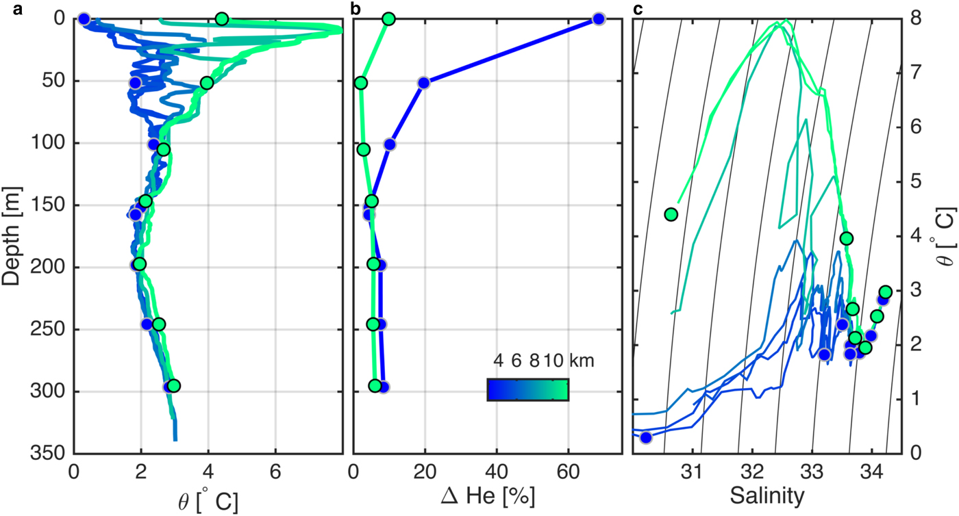
Fig. 3. Ship-based measurements along the cross-shore line north of the sill. (a) Vertical profiles of potential temperature. (b) Profiles of helium from the nearshore and offshore station expressed as the percent difference from equilibrium saturation. (c) Potential temperature-salinity curves from the section. In each panel colored dots indicate the location of the noble gas measurements, and color indicates offshore distance in km and corresponds to the location on the map in Figure 1 – blue is near the coast, green is farthest offshore.
This paper follows the methods outlined in Beaird and others (Reference Beaird, Straneo and Jenkins2015) who use temperature and salinity along with the noble gases in an Optimum Multiparameter Method (OMP, Tomczak and Large, Reference Tomczak and Large1989) to evaluate the submarine meltwater and subglacial discharge content of the proglacial waters. Briefly, the OMP uses a weighted non-negative least squares optimization routine to solve a formally overdetermined set of linear mixing equations. This is an extension of Eqn (2) that weights the properties in the matrix ${\bf A}$
according to a measure of each property's utility. Following Tomczak and Large (Reference Tomczak and Large1989), the measure of utility is taken to be the variance of the endmember tracer values (
${\bf A}$
according to a measure of each property's utility. Following Tomczak and Large (Reference Tomczak and Large1989), the measure of utility is taken to be the variance of the endmember tracer values ( $\sigma _j^2 = 1/n\sum\nolimits_{i = 1}^n (A_{ij} - A_j )^2 $
) divided by the square of the largest uncertainty of that tracer across all endmembers (ε
j,max
):
$\sigma _j^2 = 1/n\sum\nolimits_{i = 1}^n (A_{ij} - A_j )^2 $
) divided by the square of the largest uncertainty of that tracer across all endmembers (ε
j,max
):
 $$W_j = \displaystyle{{\sigma _j^2} \over {{\rm \varepsilon} _{\,j,max}^2}}. $$
The OMP solves the weighted system
 $${\bf (Ax} - {\bf d)}^{\bf T} {\bf W}^{\bf T} {\bf W(Ax} - {\bf d) = r}^{\bf T} {\bf r}$$
by minimizing the norm of the residual ( $\Vert{\bf r}\Vert^2 = {\bf r}^{\bf T} {\bf r}$
) in a non-negative least squares sense.
$\Vert{\bf r}\Vert^2 = {\bf r}^{\bf T} {\bf r}$
) in a non-negative least squares sense.
The water masses used in the OMP, the properties that define them, and the weights for the parameters, are given in Table 1. The three ambient oceanic water masses used are the Atlantic Water, Polar Water and Warm Polar Water. Because of the observed curvature of the deep portion of the θ/S curve (i.e. departure from linear mixing), two values of Polar Water are defined to better represent the observations. Helium and temperature profiles (Figs 3a, b) suggest that a layer of meltwater extends over the surface of all our observations, meaning we have not observed pure Warm Polar Water. We take the Warm Polar Water to be a linear fit in θ/S space from the Polar Water value to the point where the offshore θ/S curve bends over (green curve, Fig. 1c). Also following Beaird and others (Reference Beaird, Straneo and Jenkins2015), we define two types of submarine meltwater. These types reflect a signal of enhanced helium isotope concentrations related to basal ice. In the results we sum both types of submarine meltwater, and both types of Polar Water. Following the Monte Carlo-like methods in Beaird and others (Reference Beaird, Straneo and Jenkins2015), the spread of solutions derived from many perturbed OMP realizations is taken to be representative of the uncertainty in our estimates of the water mass fractions.
We are primarily interested in the distribution of subglacial discharge and submarine meltwater. It is important to note that our methods cannot differentiate iceberg-derived submarine meltwater from glacier terminus-derived submarine meltwater. This is because the noble gas, temperature and salinity signature of the terminus and a submerged iceberg are the same, and both types of melting can occur at high hydrostatic pressures. This ambiguity is particularly important in the Jakobshavn/Icefjord region where iceberg coverage is extensive (Fig. 1), with submerged iceberg area being at least an order of magnitude larger than the face of the glacier terminus (Enderlin and others, Reference Enderlin, Hamilton, Straneo and Sutherland2016). Similarly, subglacial discharge has properties, which are the same as cold river runoff and subaerial melt of icebergs, and cannot be distinguished from these other fresh water sources. Hydrological modeling indicates that the majority of ice-sheet meltwater in the region is routed to marine terminating glaciers (see Fig. 6 in Mernild and others, Reference Mernild2015), and thus subglacial discharge probably far exceeds river input.
The comprehensive noble gas observations are only available at discrete depths on two of the seven ship-based profiles (Fig. 3). These two profiles are the innermost and outermost of the cross-shore section. The cross-shore water mass structure suggests that the middle stations (CTD only) are a mixture of the innermost and outermost (CTD and noble gas) stations (Figs 3a, c). Therefore we extend the results of the OMP solution obtained with the noble gas data to the five intermediate CTD stations along the section north of the fjord mouth. We do not make this extension to the XCTD stations in the fjord.
One way to extend the OMP would be to statistically interpolate the noble gas data or the OMP solutions in physical space. Alternatively, the extension can be done in water mass (θ/S) space, which is well resolved by the noble gas observations. In addition, the θ/S curves from the extra CTD data provide information about mixing between regions of this space. We chose to work in θ/S space. The extension is made by defining a series of small triangular elements in θ/S space whose vertices are at noble gas observation points, and using a traditional water mass analysis in these regions. Details of the method are outlined in the Appendix.
The heavy iceberg cover inside Ilulissat Icefjord makes the fjord impenetrable by boat (Fig. 1b), thus no water samples were collected in the fjord for noble gas measurements. Without the additional tracers we cannot use the quantitative OMP methods outlined above to assess the composition of glacially modified water inside the fjord. It is common practice to identify the distribution of submarine meltwater by matching the slope of the θ/S curve to the theoretical Gade slope (Gade, Reference Gade1979), or to quantify meltwater content using a three endmember variation of Eqn (2) outlined in Jenkins (Reference Jenkins1999). We avoid that method here because the presence of subglacial discharge and multiple entrained water masses make this method ill-posed (i.e. m + 1 < n in Eqn (2)). As is frequently the case in Greenland's fjords, the ambient θ/S slope between Polar Water and Atlantic Water in this region is very close to the Gade slope (Fig. 1c), providing an illustration of the degeneracy of the θ/S-only three endmember mixing model.
However, it is possible to investigate the way in which θ/S properties differ relative to ambient waters offshore and make inferences about glacier driven water mass transformation. The assumptions used here are that both subglacial discharge and submarine meltwater cool and freshen ambient ocean waters and decrease their density such that they move vertically in the water column. We assume that inside the closed fjord changes in water mass properties relative to the waters outside are dominated by glacial modification (not temporal variability or solar insolation). To evaluate the water mass transformation in the fjord we calculated temperature anomalies on isopycnals (θ′) relative to the offshore-most CTD cast. This is simply the temperature difference between each station and the offshore station at each density: θ′ obs (σ i ) = θ obs (σ i ) − θ offshore (σ i ). The quantity θ′ is not defined for regions in the fjord near the surface where the density is lower than the surface density at the offshore station. Isopycnal temperature anomalies are a convenient way to contrast water mass characteristics because they correspond to differences in temperature and salinity through the equation of state. Comparing properties on isopycnals, rather than pressure surfaces, also reduces internal wave and temporal aliasing, and is consistent with the fact that ocean circulation is largely along, rather than across, density surfaces.
RESULTS
Glacial modification inside Icefjord
The helicopter-deployed XCTDs produce a temperature and salinity section along the axis of the fjord from the Iceberg Bank to within 3 km of the terminus of Jakobshavn Isbræ (Figs 1, 4). The fjord bathymetry is not highly resolved, but point measurements suggest that it is uniformly deep, ~800 m, inland of the bank (Holland and others, Reference Holland, Thomas, de Young, Ribergaard and Lyberth2008). Two of the XCTDs collected in this study, at 41 and 57 km from the glacier terminus, did not profile to the bottom (presumably at 800 m), but only to 300 m due to probe failure.

Fig. 4. Depth vs distance from Jakobshavn Glacier terminus sections of: (a) Surface (0–10 m) average density (black) and temperature above freezing (red); (b) potential temperature with salinity contours; and (c) isopycnal potential temperature anomaly relative to the offshore-most CTD station, with potential density contoured (not defined near the surface in the fjord where density is lower than offshore). The cross-shore ship section is plotted at the left – this section was occupied one day after the XCTD survey. Note the expanded vertical scale between the surface and 100 m in b and c. Colored triangles at the top correspond to the station location in Figure 1. Regions of no data are hatched.
The densest (σ θ ≥ 27.25 kg m−3) water mass properties in the fjord match those measured outside the fjord (Fig. 2b), consistent with the renewal of deep fjord basin by waters at sill depth, as posited by Gladish and others (Reference Gladish, Holland, Rosing-Asvid, Behrens and Boje2015b). However, much of the rest of the fjord water column properties (all but the densest waters) differ from those found offshore. The observed water mass modification suggests interaction with submarine meltwater and subglacial discharge. The θ/S properties in the fjord are within the range of possible properties described by mixing lines connecting the densest unmodified waters with the subglacial discharge and submarine meltwater (Figs 1c, 2a). The quantitative composition of these waters cannot be determined because of the possibility that up to five water masses are contained in the mixture (submarine meltwater, subglacial discharge, Atlantic Water, Polar Water and Warm Polar Water). Thus there are more unknowns (n ≤ 5) than can be formally constrained by the analysis of Eqn (2) with only temperature and salinity (m + 1 = 3). However the observed modification is consistent with the input of submarine meltwater and subglacial discharge. In many places the θ/S curves observed in the fjord match mixing lines expected to result from the addition of submarine meltwater and subglacial discharge to the ambient ocean waters (Fig. 2a).
The addition of subglacial discharge and submarine melt alters the properties of a substantial portion of the fjord water column. From the surface to 25 m depth the fjord is significantly fresher than surface waters offshore (Fig. 4b). This fresh layer creates a strong surface density gradient where the upper 10 m average density changes by 4.5 kg m–3 in 10 km across the Iceberg Bank (Fig. 4a). The fresh surface waters of the fjord are also extremely cold. Within 30 km of the terminus the upper 10 m of the fjord are at, or very near, the in situ freezing point (Figs 2a, 4a). Down to 150 m, fjord waters remain colder than waters offshore. Comparison with offshore waters of the same density indicates isopycnal temperature anomalies reaching − 8°C relative to the offshore-most ship station (Figs 4b, c). Deeper in the fjord, from 225 to 600 m (in the density range 27.05 ≤ σ θ ≤ 27.25 kg m−3) potential temperatures are warm relative to equally dense waters offshore (Figs 2b, 4c). All this evidence points to a deep-reaching modification of fjord waters by glacial buoyancy forcing.
Glacially modified water north of Icefjord
The cross-shore section is located just north of the deepest part of the sill at the fjord mouth (Fig. 1a). Fresh coastal plumes in geostrophic balance should flow with the coast to the right – northward in this case (Münchow and Garvine, Reference Münchow and Garvine1993). The Icefjord Bank is very shallow on its southern edge (50 m), inhibiting flow in that direction. Therefore, one would expect to observe the outflow of any glacially modified waters from the fjord at the occupied section. The ship survey did not include stations to the south of the fjord, so we cannot preclude some spreading of glacially modified waters in that direction. However, buoyant current dynamics suggest that flow should be to the north past the occupied section. Indeed, isopycnals tilt down toward shore, setting up a baroclinic pressure gradient consistent with northward along-shore flow of a buoyant coastal current (Fig. 5a). The upper 100 m are cold and fresh near the coast and warm progressively offshore (Figs 3a, 5a). Substantial nearly-isopycnal interleaving between cold and (relatively) fresh, and warm and (relatively) salty waters is seen along the section (Fig. 3c). Temperature and salinity in the interleaved intrusions are nearly density compensated, so that isopycnal slopes in the cross-shore direction are less steep than isohaline slopes (Fig. 5). The cold, fresh waters near shore with the lowest isopycnal temperature anomalies have relatively high turbidity (Figs 5b, c). Both the turbidity and isopycnal temperature anomaly concentrations decrease in the offshore direction. Elevated turbidity is often associated with sediments suspended in glacially modified waters providing qualitative evidence of subglacial discharge content in the shallow nearshore waters.
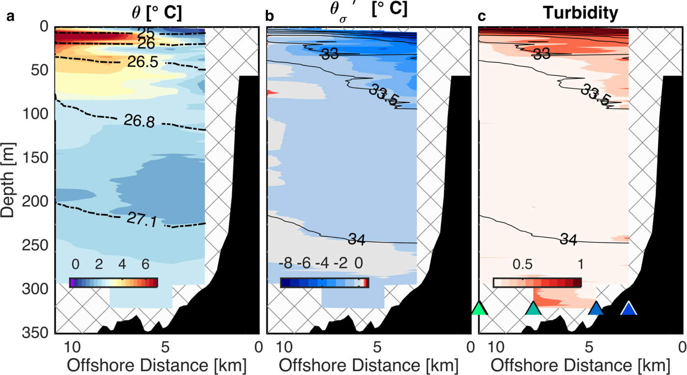
Fig. 5. Depth vs cross-shore distance sections of: (a) potential temperature with density contours; (b) potential temperature anomaly along isopycnals relative to the offshore profile with salinity contours in black; (c) water column turbidity with salinity contoured in black. The locations of the stations are indicated by the triangles in c, where the colors correspond to the map in Figure 1. Bathymetry from Schumann and others (Reference Schumann, Völker and Weinrebe2012) along the teal line in Figure 1a. Regions of no data are hatched.
These density, turbidity, salinity and temperature fields are consistent with a wedge of buoyant glacially modified water near the coast flowing north from the Icefjord Bank. More quantitative confirmation comes from the helium concentration profiles, which show supersaturations in the nearshore profile, increasing from 100 m up to the surface (Fig. 3b, blue line). Helium measurements are elevated up to 70% above equilibrium – clear evidence for submarine meltwater as a constituent of the cold fresh waters near the coast. Helium saturation anomalies are relatively low in the offshore profile, except at the surface where higher supersaturations suggest submarine meltwater is present.
Unlike the fjord XCTD stations, we took noble gas samples along the line outside the fjord. Thus, we have additional constraints on the mixing equations (Eqns (2) and (4)) and can solve for the amount of submarine meltwater and subglacial discharge present at the section. Using the OMP (Eqn (4)) with the temperature, salinity and noble gas data produces the distribution of submarine meltwater and subglacial discharge at the section (Fig. 6). At the nearshore end of the section submarine meltwater concentrations extend to 100 m depth, and reach concentrations as high as $2.5 \pm 0.12\% $
near the surface. At the same station subglacial discharge is found in the upper 80 m, reaching concentrations of
$2.5 \pm 0.12\% $
near the surface. At the same station subglacial discharge is found in the upper 80 m, reaching concentrations of $6 \pm 0.37\% $
at the surface. The submarine meltwater and subglacial discharge distributions that define the glacially modified water have a similar distribution to the independently measured turbidity signal. High concentrations of both submarine meltwater and subglacial discharge near the surface extend seaward at least 10 km to the offshore station, although the concentrations decrease offshore. The layer of submarine meltwater and subglacial discharge shoals to just 35 m depth at the offshore end of the section.
$6 \pm 0.37\% $
at the surface. The submarine meltwater and subglacial discharge distributions that define the glacially modified water have a similar distribution to the independently measured turbidity signal. High concentrations of both submarine meltwater and subglacial discharge near the surface extend seaward at least 10 km to the offshore station, although the concentrations decrease offshore. The layer of submarine meltwater and subglacial discharge shoals to just 35 m depth at the offshore end of the section.
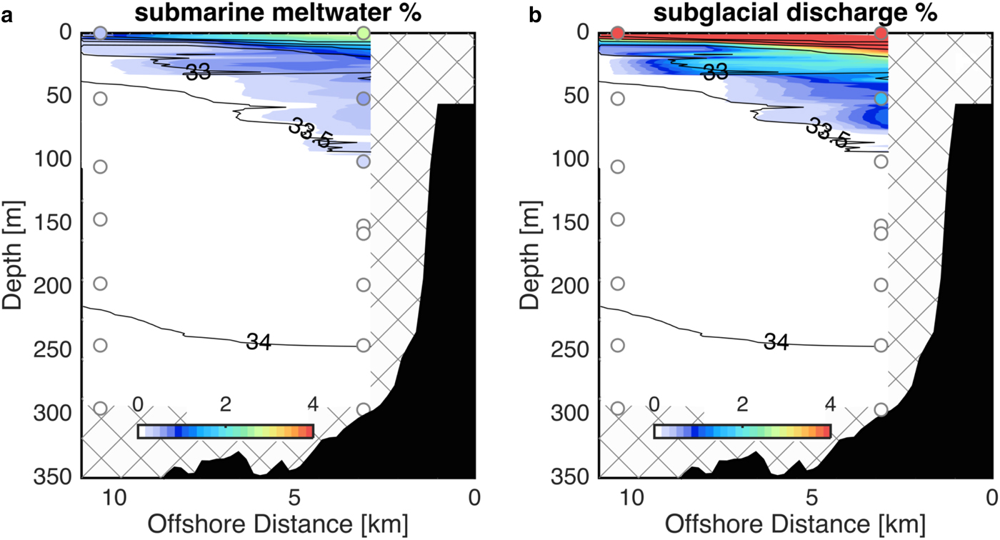
Fig. 6. Depth vs cross-shore distance sections of: (a) percent of submarine meltwater with salinity contoured in black; (b) percent of subglacial discharge with salinity contoured in black. Colored circles show the OMP solution at the locations of the noble gas observations. The color contoured field show the triangular element extension to the θ/S data. Bathymetry from Schumann and others (Reference Schumann, Völker and Weinrebe2012) along the teal line in Figure 1a. Regions of no data are hatched.
SUMMARY AND DISCUSSION
This study presents the first detailed look at the properties and distribution of meltwaters exported from Jakobshavn Isbræ and Ilulissat Icefjord. These meltwaters are derived from the runoff of ice-sheet surface ablation, of submarine melting of the glacier terminus, and submarine and subaerial melting of icebergs. The glacial meltwaters entrain and mix with ambient ocean water masses, creating a mixed, glacially modified, water mass. Characterizing and tracing glacially modified water is important because its properties and distribution determine the ice sheet's impact on the ocean.
Inside the Icefjord water mass properties are altered in ways that are consistent with fresh water forcing from melting of the glacier terminus, icebergs and runoff. The upper 150 m of the fjord are substantially colder than waters offshore, by as much as 8°C, reflecting losses to latent heat required to melt ice and to advective fluxes associated with the input of cold fresh meltwater (Figs 4b, c). The uppermost 10 m in particular are cooled to the in situ freezing point within 30 km of the ice edge (Fig. 4a). All heat available for melting has been extracted from these waters, making them incapable of contributing to further melting of icebergs. Below the surface however, substantial melting potential remains with temperatures up to 6°C above the in situ freezing point (Fig. 2a).
In the deep part of the fjord warm isopycnal temperature anomalies are found (Fig. 4c). These anomalies are consistent with the upwelling of warm dense water by buoyancy forcing at the glacier terminus (Straneo and others, Reference Straneo2011; Carroll and others, Reference Carroll2016). Assuming that these signals are the result of the glacially-driven overturning circulation, and not temporal variability, they indicate glacial modification extending to 600 m depth – deeper than has previously been shown in other large glacier/fjord systems (Johnson and others, Reference Johnson, Münchow, Falkner and Melling2011; Straneo and others, Reference Straneo2011; Heuzé and others, Reference Heuzé, Wåhlin, Johnson and Münchow2017). Without additional tracers beyond temperature and salinity, we cannot be more quantitative about the composition of the modified waters inside the fjord. Instead, we only point out that the anomalies are consistent with a deep reaching overturning circulation driven by subglacial discharge and submarine melting at depth. Gladish and others (Reference Gladish, Holland, Rosing-Asvid, Behrens and Boje2015b) suggest that this type of glacier-driven circulation could renew fjord waters over the course of a single summer, and dominates the fjord circulation over remote forcing from outside the sill.
Above 250 m in the fjord, the temperature anomalies switch from positive to negative and fjord waters become cool relative to unmodified waters offshore (Fig. 4c). These observations contrast with plume theory modeling results that predict positive temperature anomalies associated with the glacially modified waters produced by Jakobshavn Isbræ (Carroll and others, Reference Carroll2016). Carroll and others (Reference Carroll2016) find that upwelling plumes equilibrate below the surface of the fjord (in the range 50–350 m), carrying entrained warm Atlantic Waters into the cold Polar Water depth range. However, the plume model does not incorporate the impact of melting of icebergs that cover Ilulissat Icefjord (Fig. 1b). The melting of submerged iceberg keels would create a distributed network of small upwelling plumes along the icebergs throughout the fjord, and could easily explain the cold anomalies observed in the upper 150 m of the fjord (Fig. 4c). This suggests that the characteristics of the glacially modified waters exiting the proglacial fjord are not only set by processes at the glacier terminus, but also by interactions between fjord waters and the extensive iceberg cover.
Sharp gradients in properties are seen across the Iceberg Bank at the mouth of the fjord (Fig. 4a). Surface temperatures rise across the bank, though the surface temperature gradient is stronger on the offshore side of the sill. The surface density (and salinity) gradient is extremely large over the sill, setting up a pressure gradient that must drive complex circulation at the iceberg-congested sill. These changes in properties across the sill, along with observations of glacially modified waters outside of the fjord, suggest that substantial mixing must take place as glacially modified waters cross the sill and enter Disko Bay.
North of the fjord mouth, glacially modified water is found in a thick, stratified layer reaching down to 100 m near the coast (Fig. 6). The hydrographic properties of the glacially modified water vary, with salinities between 29.38 and 33.58, density in the range 1023.54–1026.77 kg m–3, and temperatures between 0.29 and 8°C. This thick layer of glacially modified water is more than 100 m above the sill depth. The maximum combined concentration of submarine meltwater and subglacial discharge is $8.5 \pm 0.5\% $
, implying that the minimum entrained ambient ocean water content is
$8.5 \pm 0.5\% $
, implying that the minimum entrained ambient ocean water content is $91.5 \pm 0.5\% $
. Thus the properties of the outflowing modified waters, including their temperature, salinity and nutrient content, are largely set by the ambient ocean waters entrained. In the case of the waters flowing out of Ilulissat Icefjord, these entrained waters are ~50% Polar Water and 40% Atlantic Water, with a varying degree of Warm Polar Water further offshore (fields not shown). The thickness of the layer, 100 m, emphasizes that the high levels of entrainment cause some portion of the vertical, meltwater-driven plumes to equilibrate below the sea surface – contributing to potential vorticity (isopycnal thickness) anomalies, but not to increased surface stratification. The modified waters form a buoyant gravity current that has turned anticyclonicly with respect to the fjord mouth. The density structure of the glacially modified waters is such that they should propagate northwards once geostrophic adjustment is complete.
$91.5 \pm 0.5\% $
. Thus the properties of the outflowing modified waters, including their temperature, salinity and nutrient content, are largely set by the ambient ocean waters entrained. In the case of the waters flowing out of Ilulissat Icefjord, these entrained waters are ~50% Polar Water and 40% Atlantic Water, with a varying degree of Warm Polar Water further offshore (fields not shown). The thickness of the layer, 100 m, emphasizes that the high levels of entrainment cause some portion of the vertical, meltwater-driven plumes to equilibrate below the sea surface – contributing to potential vorticity (isopycnal thickness) anomalies, but not to increased surface stratification. The modified waters form a buoyant gravity current that has turned anticyclonicly with respect to the fjord mouth. The density structure of the glacially modified waters is such that they should propagate northwards once geostrophic adjustment is complete.
We lack velocity observations from the 2014 cruise, therefore estimating the transport of submarine meltwater and subglacial discharge is not possible. However, we can make an approximate statement about the relative export of subglacial discharge and submarine meltwater for this summertime survey. The observed ratio of subglacial discharge content to submarine meltwater content in Figure 6 varies from 0 to 3, with an average value of 2. Assuming that the mean ratio of subglacial discharge content to submarine meltwater content in the glacially modified water is also representative of the mean ratio of the transports of those two water types, then roughly two times more subglacial discharge is exported from the fjord than submarine meltwater. We can compare this estimate to published estimates of submarine meltwater and subglacial discharge input to Ilulissat Icefjord. Enderlin and others (Reference Enderlin, Hamilton, Straneo and Sutherland2016) recently estimated the iceberg meltwater flux of the mélange in the Icefjord to be 678–1346 m3 s–1. Using a submarine melt rate of 3.5 m d–1 applied across the full terminus of Jakobshavn they estimated an additional 400 m3 s–1 of submarine meltwater production from the terminus. From the perspective of the noble gas tracers these two indistinguishable forms of submarine meltwater would amount to a total flux of submarine meltwater of 1078–1746 m3 s–1. The submarine meltwater flux can be compared with an estimated peak summer liquid fresh water runoff into all of Icefjord of ~1700 m3 s–1 from Mernild and others (Reference Mernild2015). Not all of this runoff exits below the terminus of marine terminating glaciers (i.e. as subglacial discharge), but based on hydrodynamic modeling of the region (Mernild and others, Reference Mernild2015), it is likely that much of it does. Assuming that the 1700 m3 s–1 of runoff into Icefjord is all injected as subglacial discharge, these estimates give a ratio of subglacial discharge to submarine meltwater transport in the range 1–1.6. It should be noted that there is a strong seasonality in the production of subglacial discharge, and our measurements were taken during the summer melt season. The relative impact of submarine melt and subglacial discharge should change throughout the year. While our rough estimate results in a somewhat higher ratio of subglacial discharge to submarine meltwater, it emphasizes the significant contribution of submarine meltwater even in summer to the total fresh water discharge from Greenland's glaciers – much of which is likely derived from icebergs melting in the fjord. This observation adds to a growing body of evidence that submarine meltwater, and in particular iceberg meltwater, is a large component of the fresh water budget of proglacial fjords (Enderlin and others, Reference Enderlin, Hamilton, Straneo and Sutherland2016; Jackson and Straneo, Reference Jackson and Straneo2016). Icebergs have variable keel depths and are spread horizontally throughout the fjord. The impact of this distributed buoyancy forcing on fjord circulation has not yet been investigated, but may play an important role in the buoyancy-forced fjord circulation.
The observations presented here are the first quantitative description of the characteristics of meltwaters exported from Jakobshavn Isbræ and Ilulissat Icefjord. Inside the fjord we lack the full suite of measurements, but see modification consistent with a deep overturning cell driven by buoyancy forcing at depth. Outside the fjord we find a thick, meltwater-laden, wedge of glacially modified water north of the fjord mouth with the form of a buoyant coastal current. Noble gas tracers fully determine a system of linear equations that describe the mixture of waters that produce the glacial outflow. Subglacial discharge and submarine meltwater are found in a ratio of roughly two to one. The vast majority of the glacially modified waters are made of entrained ambient ocean water types. Glacial-origin fresh water is found at depth where it contributes to isopycnal thickness anomalies, rather than increased surface stratification. The observations are first steps toward an observational understanding of the fate of Greenland's meltwater and its interaction with regional and large-scale ocean circulation.
SUPPLEMENTARY MATERIAL
The supplementary material for this article can be found at https://doi.org/10.1017/aog.2017.19.
ACKNOWLEDGEMENTS
We appreciate the helpful comments of the editor and three reviewers who contributed to an improved manuscript. We thank Dempsey Lott and Kevin Cahill their laboratory expertise, Rebecca Jackson for expertise in the field and helpful analysis discussions. We gratefully acknowledge support from WHOI's Ocean and Climate Change Institute, the WHOI Doherty Postdoctoral Scholarship, the US National Science Foundation grant NSF OCE-1536856, and the leaders and participants of the Advanced Climate Dynamics Summer School (SiU grant NNA-2012/10151). Ship-based CTD data are freely available from the NOAA National Centers for Environmental Information, discoverable with Accession Number 0162649. Expendable CTD data are included in the Supplementary Material. Noble gas data are freely available at the Biological and Chemical Oceanography Data Management Office (BCO-DMO, http://www.bco-dmo.org/).
APPENDIX
EXTENSION OF NOBLE GAS OMP SOLUTIONS TO CTD DATA
The noble gas data are only available at discrete locations (Fig. 3c), though these locations span the range of water mass space. We therefore attempt to extend the OMP analysis to all the ship-based CTD data. We use a traditional three-endmember water mass analysis in local regions to fill in the gaps in θ/S space. The extension is made by defining a series of non-overlapping triangular elements in θ/S space whose vertices are at noble gas observation points (Fig. 7). We assume that within these regions local mixing sets properties and therefore points inside each bounded region can be written as a combination of the properties at the vertices – as in classical water mass analysis. We can then use temperature and salinity in Eqn (2) to solve for the fraction, p k (with k = 1,2,3), of each vertex, v k (equivalent to a local endmember with properties θ k and S k ), contained in the mixture observed at each interior point (θ obs , S obs ):
 $$1 = p_1 + p_2 + p_3$$
 $$\theta _{obs} = p_1 \theta _1 + p_2 \theta _2 + p_3 \theta _3$$
 $$S_{obs} = p_1 S_1 + p_2 S_2 + p_3 S_3$$
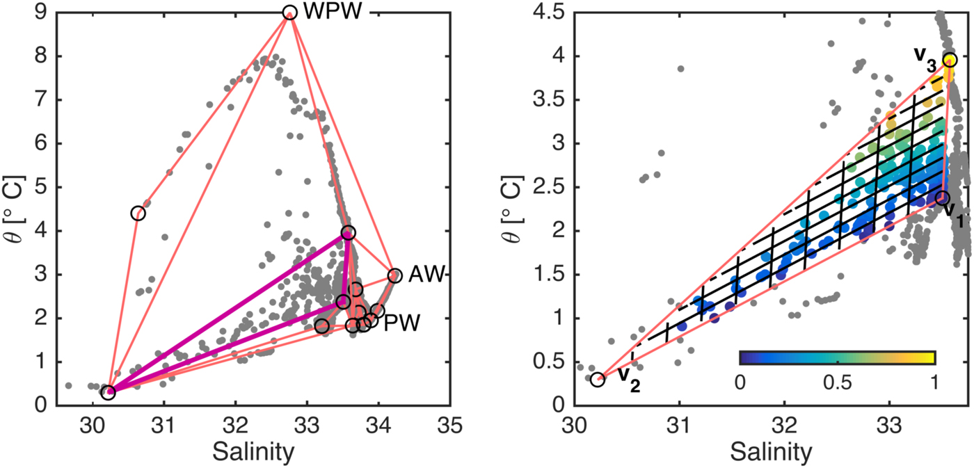
Fig. 7. Left: Potential temperature vs salinity plot of ship-based CTD observations (gray dots), noble gas sample points (black circles) and triangular elements (pink lines) for the three-endmember method to extend noble gas OMP solutions to all CTD data. Right: an example of a single triangular element (magenta in left panel). Black lines show the composition grid for the concentration of vertices v 2 and v 3 from Eqns (A1)–(A3). Colored dots show the concentration of vertex v 3 at each CTD observation.
The solution to the equations above gives a set p k for each observation in the bounded region. This method assumes that the water mass analysis is evenly determined by temperature and salinity (i.e. m + 1 = n) within each bounded region. The set of 15 bounding regions used are shown in Figure 7, along with a geometric representation of Eqns (A1)–(A3) in a sample region. The defined Warm Polar Water endmember has been added as a vertex to enclose the warm surface waters offshore.
Next, because the water mass fractions (f i , Eqn (1)) at each of the vertices (v 1, v 2, v 3) are known (from the noble gas OMP solution, Eqn (4)), we can reconstruct the water mass fractions at each interior point:
 $$f_i^{obs} = p_1 f_i (v_1 ) + p_2 f_i (v_2 ) + p_3 f_i (v_3 )$$
In summary: first we find the relative contribution of each vertex to a given observation point in θ/S space (a three-endmember mixing model), then we use the fact that we know the water mass content of those vertices (from the noble gas OMP) to derive the water mass content at the observation location. A few points cannot be bounded by the noble gas defined vertices. For those few points 2-D linear interpolation is used.
This three-endmember method is subject to the same caveats that are discussed in the text: it will fail if points in a triangular element are the product of the interaction of more endmembers than just the three vertices that define the element. In that case the system is underdetermined by temperature and salinity observations and errors in interpretation could arise. In the limited use described here – ‘interpolating’ from the noble gas samples only onto CTD data points on the section north of the fjord mouth – we believe the assumptions are justified. The section is away from the glacier, and thus glacier-driven water mass transformation. We assume that local mixing between water masses sets properties on the section.


 Open access