


INTRODUCTION
Many countries producing food from animals are recording the spatial location of farms. This information is of great use for disease surveillance and control and in the event of outbreaks of infectious diseases (e.g. avian influenza and foot-and-mouth disease). Spatial information (e.g. herd location) along with details of the animal population (e.g. herd type, herd size, etc.) can be used to develop models that quantify the effects of factors influencing the presence or absence of disease at a given location (e.g. endemic diseases such as salmonellosis).
Median polish is a general procedure used to remove trends and reduce large-scale variation in (regular) lattice data [Reference Cressie1–Reference Cressie and Glonek3]. Median-based residuals are calculated by removing column and row medians. In the original formulation by Tukey [Reference Tukey2] this was done repeatedly until convergence. In geostatistics, trends lead to a steadily increasing semivariogram. Large-scale variations often cause a large non-spatial variation (nugget effect) and a small spatial variation (partial sill). Such a procedure is commonly used in the field of time-series analysis before fitting stationary models to the data. There are also resemblances between median polish and the so-called lowess or loess (robust locally weighted) regression model suggested by Cleveland [Reference Cleveland4].
For irregularly spaced data, Cressie [Reference Cressie1] suggested drawing a low-resolution map of the spatial locations. In practice, this can be done by overlaying a grid onto the high-resolution map and assigning data locations to the nearest grid node. If large-scale variation and trends are considered to be in columns and rows, this procedure can be used to calculate median polish residuals for irregularly spaced data. However, in many cases removing row and column effects is unnatural. Often the nuisance effects tend to be more regional in nature. For instance they might be the result of soil properties or regional practices such as manure handling or veterinary practice effects. Such effects are not always easy to model or estimate in traditional ways.
Ersbøll & Nielsen [Reference Ersbøll and Nielsen5] estimated the range of influence between cattle herds of relevance for local spread of Salmonella Dublin in Denmark. S. Dublin herd status was a binary variable of high/low antibody levels to S. Dublin in bulk-tank milk and blood samples collected from all cattle herds in Denmark. Deviance residuals were calculated based on a generalized linear model. The range of influence was estimated based on the deviance residuals using an exponential semivariogram. Due to large regional differences the range of influence was estimated for each region separately. Furthermore, a large non-spatial variation (nugget effect in the semivariogram) was obtained compared to the spatial variation. Non-spatial variation could be due to, e.g. veterinary practice, herd type and herd size.
The aim of the current study was to develop a generic detrending procedure for irregularly spaced locations in order to remove large-scale variation. A regional polish procedure was therefore developed.
An application to S. Dublin in Denmark is described. Regional polish was used to eliminate regional effects in order to improve the estimate of the range of influence. Hereby, the range of influence was estimated for a large region as a whole with less variation compared to the estimates obtained without prior use of the regional polish procedure.
METHODS
Regional polish
Procedure
As an example we considered analysis of variance (ANOVA) which basically consists of assessing an expected value in a cell and a random error. Analysis consists of estimating these expected values, usually by estimating parameters in the model by least squares and assigning any remaning variance to random error. Tukey [Reference Tukey2] introduced the method of median polish as an alternative method to estimate the expected values. Equivalent to a two-way ANOVA row medians and column medians are removed. This process is often repeated until convergence.
In geostatistics we considered data in a spatial layout where the data are expected to display some kind of spatial dependency. Data at a certain geographical position is often considered as having an expected value and a random error. Both these components may be spatially dependent in which case the expected values would constitute a trend surface which could be removed before further analysis on the random component. A very common type of spatial analysis is estimation of the so-called (semi)variogram.
Unless other precautions are taken the semivariogram is sensitive to trends in data (non-stationarity). The semivariogram will not reach a stable value and it may become difficult or impossible to estimate and interpret. Trends are therefore often removed before further analysis. This can be done in a large number of ways. An especially simple geographical layout is for the data to be on a lattice grid. The traditional example is data from a field experiment, but the spatial layout of experimental rats in cages could be another. In that case median polish could be one such possibility of trend removal.
Regional polish is developed as an alternative to remove large-scale variation and trends in irregularly spaced data. Regional polish residuals are obtained by calculating weighted medians based on observations in the neighbourhood. For each herd location, an inverse distance weighted median was calculated for observations from herds in the neighbourhood. The regional polish residuals were obtained as the difference between the observed value and the weighted median value for each herd. The size of the neighbourhood used to calculate medians should be large enough for it to be still possible to estimate small-scale spatial variation within the distance. The weighting scheme introduces the spatial element into the procedure. Intuitively, the weights should be high close to the location in question and drop-off for increasing distances. This can be elaborated in a large number of ways. In our case a simple inverse distance weight function was used to estimate the median within the neighbourhood. Moreover, we only performed one pass of the regional polish procedure. In line with the proposal by Tukey [Reference Tukey2] it is possible to iterate the procedure a number of times.
Weighted median
A weighted median is the median value of the observations when taking into account the weights of the observations. Consider five observations with values 1, 2, 3, 4, 5. The ordinary median is 3.
The weighted median of the values 1, 2, 3, 4, 5 with the corresponding weights 1, 2, 1, 2, 4 can be illustrated intuitively by duplicating the values according to the weights giving 1, 2, 2, 3, 4, 4, 5, 5, 5, 5.
The usual definition of the median would then give the value 4.
However, rather than duplicating values it is more efficient to look at the weights themselves. First we normalize the weights to sum to 1 as 0·1, 0·2, 0·1, 0·2, 0·4.
The weighted median is now found by cumulating the weights from the lowest value (1) until the cumulated weight equals or exceeds 0·5.
The corresponding number is the weighted median. In the case above this happens at the value 4, where the cumulative weight is 0·6.
The direct (unweighted) median of the values 1, 2, 3, 4, 5 may be seen as a special case of a weighted median simply by using equal weights 0·2, 0·2, 0·2, 0·2, 0·2.
Further considerations concerning the weighted median can be found in Yin et al. [Reference Yin6].
Regional polish procedure
As an example consider a herd (herd V) with four neighbouring herds (herds I–IV) (Table 1). In order to find the weighted median value of herd V an inverse distance weight function is used [1/(1+d), where d is a unit of distance]. The cumulated weight equals or exceeds 0·5 corresponding to the value 4 which is the weighted median. An ordinary (unweighted) median would give the value 3.
Table 1. Illustration of the algorithm used to calculate the weighted median of herd V
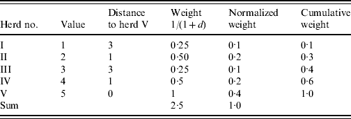
d represents a unit of distance.
We note that the weighted median in this case favours the spatially closer-lying value. When applying the regional polish procedure to real datasets different sizes of the neighbourhood for estimating the weighted median (maximum distance) should be evaluated. Furthermore, different weighting functions could be considered [e.g. 1/(1+d) and 1/(1+d)2, where d is a unit of distance]. The size of the neighbourhood and the weighting functions should be evaluated in relation to the estimate and standard error of the parameter in question.
Application: S. Dublin in cattle herds
All registered cattle herds in the Jutland peninsula in 2003 (n=20 099) were included in the study. S. Dublin herd status was either positive (having a high serological response using blood and bulk-tank milk samples) or negative. In total, 10% of the herds had a positive S. Dublin herd status (Fig. 1). (For more details, see Ersbøll & Nielsen [Reference Ersbøll and Nielsen5].) The aim of the study was to estimate the range of influence between cattle herds with a positive S. Dublin herd status. The range of influence is the average distance between herds where locations are no longer correlated regarding S. Dublin herd status. The range of influence is of interest for control and eradication programmes, e.g. for the determination of the radius of protective zones around infected herds. Ersbøll & Nielsen [Reference Ersbøll and Nielsen5] used deviance residuals obtained from a generalized linear model with a binomial distribution. Herd size and herd density were included in the model. A semivariogram for Jutland was modelled based on the deviance residuals. However, the semivariogram based on the deviance residuals for Jutland increased steadily and the range of influence could not be estimated. Due to large differences between the six different regions in Jutland, deviance residuals and semivariogram parameter estimates were obtained for each region, separately (Fig. 2, Table 2). The range of influence estimated for three of the six regions were not significantly different from zero due to a large standard error.

Fig. 1. Geographical distribution of Salmonella Dublin-seropositive herds in the Jutland peninsula, Denmark, 4th quarter 2003. (For abbreviations see Table 2.)
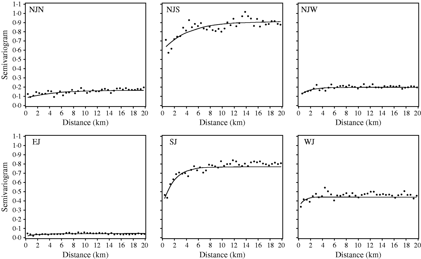
Fig. 2. Empirical (•) and fitted (—) robust semivariograms for Salmonella Dublin herd status using deviance residuals in six regions. (For abbreviations see Table 2.)
Table 2. Estimates of the range of influence (km) between cattle herds with positive Salmonella Dublin herd status
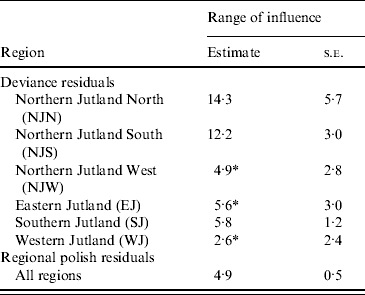
* The range of influence is not significantly different from 0.
In order to estimate the range of influence for Jutland with less variation the regional polish procedure was applied to reduce the effect of the large-scale variation.
The range of influence between cattle herds with a positive S. Dublin herd status was estimated in the current study based on regional polish residuals. The robust semivariogram estimator suggested by Cressie & Hawkins [Reference Cressie and Hawkins7] was used
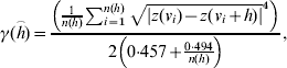
where γ(h) is the semivariogram, h is the distance between herd location, z(v) is the residual value (deviance residual or regional polished residual) at location, v and n(h) is the number of pairs of herds in distance h.
An exponential semivariogram model was fitted given as
where c 0 and c are the nugget effect and partial sill and a′=3 a is the practical range of influence.
Regional polish residuals were obtained using the procedure as described with the further restriction of a maximum distance of 10 km (corresponding to weight 0 at greater distances). The restriction has the practical consequence of reducing the computational burden. A semivariogram was estimated based on the regional polish residuals (Fig. 3). The semivariogram model based on the regional polish residuals resulted in a range of influence estimated at 4·9 km (s.e.=0·5 km) (Table 2, Fig. 4).

Fig. 3. Maps (inverse distance weighted) of (a) deviance residuals, (b) trends and (c) regional polish residuals.
Different sizes of the neighbourhood (maximum distance) for estimating the weighted median were evaluated ranging from 5 km to 40 km. With a maximum distance of 5 km the range of influence was estimated at 3·9 km. This maximum distance is considered too short, as the range of influence is of the same size as the maximum distance. When increasing the maximum distance to 10, 20 and 40 km the range of influence was estimated at 4·9–5·5 km.
The regional polish residuals effectively reduce the large-scale variation. A semivariogram can be estimated for all six regions in Jutland together (Fig. 4). This was not possible when using the deviance residuals without regional polish. The standard error of the range of influence parameter estimate was small (0·5 km) compared to the similar standard errors for the range of influence parameter estimates for each of the six regions separately (min–max: 1·2–5·7 km).
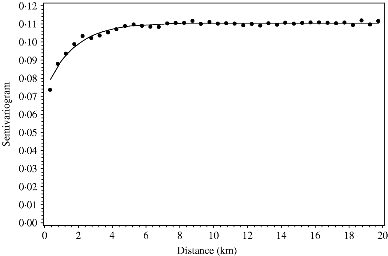
Fig. 4. Empirical (•) and fitted (—) robust semivariogram for Salmonella Dublin herd status using regional polish residuals for all herd locations in all regions in Jutland.
DISCUSSION AND CONCLUSION
For regularly spaced (gridded) data the well-known median polish algorithm is traditionally used. Here we have developed an alternative for irregularly spaced data called the regional polish algorithm. It is performed by calculating a weighted median of each data-point in turn. The original data-point is adjusted by subtracting the weighted median value. The result is called the regional polished residual.
The following issues should be considered when using the above-mentioned procedure. First, the size of the neighbourhood should be large enough to retain the small-scale variation in the regional polished residuals, but small enough to remove the large-scale trends. This is implemented through the weighting scheme. In our case we used a simple inverse distance weighting scheme. In order to reduce the computational burden we placed a further restriction of not including data-points further away than the selected maximum distance (in the example we chose 10 km). This is equivalent to weight 0 at larger distances. Second, the number of iterations performed needs to be determined. In the original formulation by Tukey [Reference Tukey2] it is suggested to continue the median polish procedure alternating over rows and columns until small or no further changes are observed. This is also possible for the regional polish scheme simply passing over the residuals from the previous iteration until small or no further change occurs. However, in our case we achieved very satisfactory results with only one iteration.
When comparing the original formulation of the median polish algorithm with regional polish the first is obviously not isotropic since it is used on specific directions, i.e. rows and columns. Depending on the weighting scheme and the actual spatial layout of data-points, the regional polish algorithm can more closely approximate isotropy.
The algorithm has successfully been applied to S. Dublin data containing large-scale trends. In previous work by Ersbøll & Nielsen [Reference Ersbøll and Nielsen5] the data were analysed in several different regions in order to avoid problems with large-scale trends. By using regional polish this was circumvented and stable estimates of the geostatistical parameters were achieved.
DECLARATION OF INTEREST
None.


