


INTRODUCTION
The glaciers in the Himalaya constitute the third largest ice mass in the world after the Arctic and Antarctic regions. Rivers originating from these glaciers are the primary source of water to the population downstream. The amount and timing of melt from these glaciers are strongly related to local precipitation and temperature (Barnett and others, Reference Barnett, Adam and Lettenmaier2005). Recent studies in the Himalaya suggest that glacier melting could accelerate in the future due to climate change (Immerzeel and others, Reference Immerzeel, van Beek, Konz, Shrestha and Bierkens2012; Chaturvedi and others, Reference Chaturvedi, Kulkarni, Karyakarte, Joshi and Bala2014; Lutz and others, Reference Lutz, Immerzeel, Shrestha and Bierkens2014; Shea and others, Reference Shea, Immerzeel, Wagnon, Vincent and Bajracharya2015). The persistent mass loss of the glaciers could lead to retreat in glacier area until a new equilibrium with climate is achieved. It will further affect runoff from the glaciers, i.e. runoff may increase during the initial decades of climate warming and then decline near the end of the century (Huss and others, Reference Huss, Farinotti, Bauder and Funk2008; Immerzeel and others, Reference Immerzeel, van Beek, Konz, Shrestha and Bierkens2012). In addition to changing climate, the growing population of the region also demands a proper management of water resources. Therefore, knowledge of annual variations in glacier-stored water is important for planning water resource management in this region. Trends and variability in glacier-stored water can be inferred by monitoring glacier mass balance at basin scale in conjunction with local climate.
Mass balance is a measure of difference between the input and output of water stored in a glacier over a balance year (Paterson, Reference Paterson2000). Hence, mass-balance information on multiple spatial and temporal scales can provide a perspective on glacier interactions with hydrology and climatology in mountainous terrain. There are direct and indirect methods of estimating glacier mass balance. Direct measurements of mass balance are glacier-specific. Indirect measurement methods such as geodetic, gravimetric and accumulation-area ratio (AAR) are widely used to analyse mass balance at larger scales in the Himalaya (Kulkarni and others, Reference Kulkarni, Rathore and Alex2004; Berthier and others, Reference Berthier2007; Matsuo and Heki, Reference Matsuo and Heki2010; Brahmbhatt and others, Reference Brahmbhatt2011; Gardelle and others, Reference Gardelle, Berthier, Arnaud and Kääb2013; Vincent and others, Reference Vincent2013; Mir and others, Reference Mir, Jain, Arun and Goswami2014). Among these, the geodetic method is often used to estimate region-wide long-term mass balance (Berthier and others, Reference Berthier2007; Gardelle and others, Reference Gardelle, Berthier, Arnaud and Kääb2013; Vincent and others, Reference Vincent2013; Vijay and Braun, Reference Vijay and Braun2016). However, the geodetic method has limitations: it may not produce annual variations in mass balance due to uncertainties and availability of digital elevation models (DEMs). The satellite-based gravitational method can provide annual mass balance for a large area but with coarser spatial resolution (~400 km). The AAR method provides an option to calculate mass balance with a higher temporal resolution at individual glaciers, which can then be scaled up to provide basin-wide mass budget. However, cloud cover, sporadic snowfalls and data gaps in satellite images hamper the mass-balance estimates using the AAR method (Kulkarni, Reference Kulkarni1996; Rabatel and others, Reference Rabatel, Dedieu and Vincent2005; Tawde and others, Reference Tawde, Kulkarni and Bala2016).
To circumvent the challenge of locating equilibrium line altitude (ELA) in the AAR method, Tawde and others (Reference Tawde, Kulkarni and Bala2016) have suggested a new approach. The improved AAR method discussed by Tawde and others (Reference Tawde, Kulkarni and Bala2016) models annual changes in ELA (altitude where the total melt and accumulation over a balance year are equal) using snowfall measurements and a temperature-index (TI) model. The model-derived annual ELA and AAR are then used to estimate specific mass balances of glaciers by employing the AAR/mass-balance relationship for the basin. Compared with the traditional AAR method, the method discussed by Tawde and others (Reference Tawde, Kulkarni and Bala2016) reduces the bias between modelled and field mass-balance estimates by up to 50.44%.
In Tawde and others (Reference Tawde, Kulkarni and Bala2016), we have applied and tested the improved AAR method for a few glaciers in the Chandra basin. In the present analysis, we extend the method to the entire basin. One can use the more complex enhanced temperature-index (ETI) or energy-balance (EB) models instead of the TI model to estimate snowmelt (Hock, Reference Hock1999; Pellicciotti and others, Reference Pellicciotti2005; Favier and others, Reference Favier2011; Carenzo, Reference Carenzo2012). However, previous studies have found that the improvement in melt estimates using ETI models is not significant and both ETI and EB models need more in situ input data and parameters from glaciers to estimate melt (Blard and others, Reference Blard2011; Gabbi and others, Reference Gabbi, Carenzo, Pellicciotti, Bauder and Funk2014). Therefore, the TI model is preferred in the present study because of its efficiency in estimating melt with simple computations and minimal input requirements. The main goal of this study is to use the improved AAR method and estimate mass balance at larger spatial scale over a period of 28 years. We compare our model-derived mass balance with the geodetic method at basin scale and with the regional–global glacier mass-balance trends. The sensitivity of basin-wide mass balance to climate is also discussed. Further, we estimate the glacier ice volume to examine glacier-stored water in the basin.
STUDY AREA
The Chandra basin is located in the Lahaul–Spiti district, western Himalaya, India. The basin covers an area of 2.44 × 10³ km2 with elevation extending from 2800 to 6600 m a.s.l. The glaciated area of the basin is 703.64 km2, i.e. ~30% of the total basin area (Sangewar and Shukla, Reference Sangewar and Shukla2009). There are 201 glaciers in the basin, only five of which have an area >20 km2 (Fig. 1). The basin consists of valley- and mountain-type glaciers. Most of the glaciers in the basin face north, northeast and northwest. The mean slope of glaciers in the basin is ~21°. The meteorological station near the basin suggests that the basin climate is influenced by both western disturbances in the winter and monsoon circulation in the summer (see Supplementary information). However, glaciers in the basin predominantly receive accumulation in the form of snow in the winter (October to April) (Azam and others, Reference Azam2014b; Tawde and others, Reference Tawde, Kulkarni and Bala2016).

Fig. 1. Geographical location of the Chandra basin, Lahual–Spiti district, Himachal Pradesh. The triangle represents meteorological stations, i.e. Kaza and Patseo (Snow Avalanche and Study Establishment) station. The selected glaciers (area >0.5 km2) are shown with black borders. The glaciers selected for calculation of precipitation gradient by Tawde and others (Reference Tawde, Kulkarni and Bala2016) are shown in the orange boundary.
DATA
The implementation of the mass-balance model described by Tawde and others (Reference Tawde, Kulkarni and Bala2016) requires daily/monthly measurements of temperature and precipitation at a nearby station. In the present study, daily minimum, maximum air temperature and snowfall from 1984 to 2012 are obtained from Kaza weather station (3600 m a.s.l.). Both the Chandra basin and Kaza station are located in the orogenic interior of the Himalaya. The station is ~25 km from the basin boundary (Fig. 1). Climatologically averaged annual temperature at Kaza is 3.2 °C and precipitation is 1.34 mm d−1. Other variables, such as temperature lapse rates and snow densities for calculating melt factors, are obtained from observations made at the Patseo (Snow Avalanche and Study Establishment, SASE) observatory in the same valley (Table 1). Estimated lapse rates (7.7–9.1 °C km−1) are higher than the moist adiabatic lapse rate (~6.5 °C km−1) because there is likely less water vapour at high altitudes in the orogenic interior of the Himalaya. The precipitation gradient is taken from Tawde and others (Reference Tawde, Kulkarni and Bala2016) and is derived using data on 12 glaciers in the basin (Fig. 1).
Table 1. List of input parameters used for the Chandra basin
The parameters are adopted from Tawde and others (Reference Tawde, Kulkarni and Bala2016).
The glacier boundaries used in the present analysis are from the Randolph Glacier Inventory version 5 (RGI v5). According to the inventory, the area of polygons in the basin ranges from 0.05 to 112.36 km2. However, to reduce uncertainty in discrimination of glaciers and perennial snow, only polygons with an area >0.5 km2 (146 glaciers out of 201) are selected. These glaciers account for 93% of the total glaciated area in the basin, so the exclusion of remaining polygons (area <0.5 km2) in our analysis is unlikely to alter the basin-wide mass balance. The topographic information on the selected glaciers is calculated from the Advanced Spaceborne Thermal Emission and Reflection Radiometer (ASTER) Global DEM.
METHODOLOGY
In the present analysis, we estimate (1) the glacier mass balance of the Chandra basin from balance year 1984/85 to 2011/12 (hereafter referred as 1984–2012), (2) the sensitivity of basin-wide mass balance to climate variables and (3) the volume of water stored in the basin.
Model description
We estimate basin-wide mass balance using the improved AAR method discussed in detail in Tawde and others (Reference Tawde, Kulkarni and Bala2016). Here we provide only a brief description of the method. The approach involves two major steps: (i) estimation of ELA using climate data and (ii) estimation of glacier mass balance using the AAR/mass-balance relationship.
The position of the ELA is estimated by monitoring the position of transient snowlines throughout the ablation season. To model the movement of the snowline, we need the altitudinal distribution of snowmelt and accumulation during the balance year. The altitudinal distribution of ablation at every 50 m elevation interval on glaciers is estimated using the TI model. At any altitude j, the cumulative snow ablation M j (mm) is given by
 $$M_j = \mathop \sum \limits_{i{\rm = 1}}^{{\rm \;} n} F_{{\rm snow,}i{\rm,} j} \times {\rm PD}{\rm D}_{i{\rm,} j},$$
where PDD i,j is positive degree-days (°C) and F snow,i,j is snowmelt factor (mm °C−1 d−1) on the ith day at the jth elevation zone. Snowmelt factors increase as temperatures increase above freezing point at respective elevation zones (Table 1). The summation in Eqn (1) is over all days (1 to n) in summer (May to September). May is included in the summer season because, occasionally, disappearances of snow at glacier tongues are observed in the basin at the end of May.
The altitudinal accumulation (Acc j ) of snow at different elevation zones (j) is simulated using snowfall observations and vertical precipitation gradient as follows:
 $${\rm Ac}{\rm c}_j = \mathop \sum \limits_{i = 1}^m \left( {P_{{\rm STN,}i} + \left( {P_{{\rm STN,}i} \times \displaystyle{{P_{{\rm grad}}} \over {100}} \times \Delta z} \right)} \right),$$
where P STN, i is daily snowfall recorded at the meteorological station (mm), P grad is precipitation gradient (% m−1) and Δz is the elevation difference between the particular band (j) and the meteorological station. The summation is over all days (1 to m) in winter (October to April). Here we use the mean P grad value derived from 12 glaciers (Table 1). The detailed methodology to calculate precipitation gradient is described in Tawde and others (Reference Tawde, Kulkarni and Bala2016).
The elevation at which the estimated snowmelt during the summer equals the winter snow accumulation at the end of the balance year is considered as the ELA. Based on the position of the ELA and the hypsometry of glaciers, the AAR is calculated. Further, the mass balance is calculated using the regression between AAR and mass balance. The regression relationship between model-derived AAR and field-derived mass balance over Chhota Shigri Glacier obtained by Tawde and others (Reference Tawde, Kulkarni and Bala2016) is modified here since data are now available for a longer period. The station data are now available up to 2012 and were available only up to 2009 in our previous study. The modified regression (r 2 = 0.84) using mass-balance estimates for the periods 1987–89 and 2002–12 is:
 $$ B= 186{\rm. 3} \times {\rm AAR - 122}{\rm. 8,}$$
where B is the annual specific mass balance (cm w.e.) of the glacier. As Chhota Shigri Glacier is found to represent the entire basin (Vincent and others, Reference Vincent2013; Pandey and others, Reference Pandey, Ali, Ramanathan, Champati ray and Venkataraman2016), the same regression is applied to all glaciers for the estimation of basin-wide mass balance.
The uncertainty in modelled mass balance is calculated considering two main components: uncertainty in (i) ELA and (ii) AAR. Uncertainty in modelled ELA is due to the independent uncertainties in temperature (±0.1 °C), snowfall (±2%), temperature lapse rates (±0.5 °C km−1), precipitation gradient (50% of the value, i.e. ±0.10% m−1), snowmelt factor (±0.3 mm °C−1 d−1) and DEM (±11 m). One parameter at a time is changed, keeping others constant to calculate the uncertainty due to that parameter. Uncertainty in AAR estimate depends on independent uncertainties in model-derived ELA, glacier boundaries (±5%, Pfeffer and others, Reference Pfeffer2014) and changes in glacier area over the study period (±2.5%, Pandey and others, Reference Pandey and Venkataraman2013a). Besides the uncertainty in the estimation of ELA and AAR, uncertainty in the modelled mass balance also depends on the uncertainty in glaciological observations used to derive the AAR/mass-balance regression (±0.4 m w.e. a−1, Azam and others, Reference Azam2012) and the usage of the same regression for other glaciers (±0.01 m w.e. a−1, Tawde and others, Reference Tawde, Kulkarni and Bala2016). In the present analysis, uncertainty in mass balance is given by running the model for all years and glaciers in the basin.
Volume estimation
The volume of the basin is estimated using the slope-dependent method described by Haeberli and Hoelzle (Reference Haeberli and Hoelzle1995). The reasons for preferring the slope-dependent method are the simplicity of the parameterisation scheme and the comparability of the results from this method with other ice-thickness distribution models over the western Himalaya (Frey and others, Reference Frey2014). The geometric parameters needed for the slope-dependent method are calculated from the DEM (Frey and others, Reference Frey2014). The average ice depth along the central flowline (h t) in metres is estimated as
 $$h_{\rm t} = \displaystyle{\tau \over {\,f\rho g\;\sin (\alpha )}} $$
where τ is the mean basal shear stress along the central flowline, f is the shape factor for valley glaciers (0.8), ρ is ice density, α is slope and g is the gravitational acceleration. The average thickness of glaciers (h t) is estimated assuming semi-elliptical cross-section geometry. The volume is determined by multiplying h t by the total surface area of the glacier. The uncertainty in volume is estimated using fractional uncertainty for Eqn (4) (Taylor, Reference Taylor1982). The uncertainties in f, ρ and τ are taken as ±0.1, ±10% (90 kg m−3) and ±28 kPa (SD considering all glaciers), respectively. The uncertainty in slope α is taken as the RMSE between DEM-derived-corrected slopes (Frey and others, Reference Frey2014) and slope using arctan (ΔH/l), where ΔH is the difference between the maximum and minimum elevation of the glacier and l is the glacier length along the longest flowline. The basin-wide volume is represented in gigatonne w.e. (Gt w.e.).
RESULTS
Mean ELA and mass balance
As the climate data are available from 1984 to 2012, we assess the variations in ELA and mass balance of the basin for this 28-year period. ELA of the basin varies interannually from 4825 to 6425 m a.s.l., with a model uncertainty of ±130 m (Fig. 2). The mean ELA of the basin is estimated at 5460 ± 130 m a.s.l., with an SD of ±420 m. The trend in ELA suggests that it is increasing at a rate of 113 m decade−1 (significant at 73%) (Fig. 2). The mean AAR of the basin during 1984–2012 is calculated as 34 ± 10%.
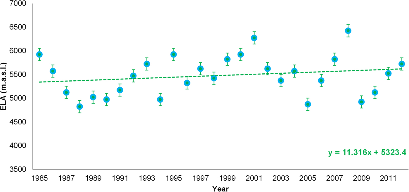
Fig. 2. Annual variations in modelled ELA of the Chandra basin from 1984 to 2012. Filled circles represent annual mean ELA (m a.s.l.) averaged over all glaciers in the basin. The uncertainty in model-derived ELA is ±130 m. The dashed line indicates the trend in ELA, i.e. +113 m decade−1 (significant at 73%).
Mean mass balance of the Chandra basin is expressed for individual glaciers, years and in terms of area-weighted value during 1984–2012. The area-weighted mean mass balance of the basin is −0.61 ± 0.46 m w.e. a−1. The mean mass balance of an individual glacier varies from −1.22 ± 0.46 to 0.01 ± 0.46 m w.e. a−1 (Fig. 3). The most negative mass balance is calculated for glaciers in the mean altitudinal range 4172–4746 m a.s.l., while the range is between 5565 and 5650 m a.s.l for glaciers with the least negative mass balance.

Fig. 3. Spatial distribution of modelled mean mass balance (m w.e. a−1) of glaciers in the Chandra basin from 1984 to 2012.
Interannual variations in area-weighted mass balance of the basin range from −1.22 ± 0.46 to +0.28 ± 0.46 m w.e. a−1 (Fig. 4). A decreasing mass-balance trend of 0.11 m w.e. a−1 decade−1 (significant at 75%) is observed. The time-series analysis of glacier mass balance suggests a mass-balance rate of −0.37 ± 0.46 m w.e. a−1 during the first decade of the study period (1984–94). In the second decade (1994–2004), a mean mass balance of −0.95 ± 0.46 m w.e. a−1 is observed, indicating acceleration in mass loss. In the third period (2004–12), the mass loss continues at a rate of −0.46 ± 0.46 m w.e. a−1. However, for a few years, i.e. 1988–90, 1994, 2005 and 2009, we find basin-wide positive mass balance which is mostly associated with a positive anomaly in winter snowfall and a negative anomaly in summer temperatures (Fig. 4). After de-trending the data, we find correlation coefficients of +0.80 and −0.66 (at 99% confidence interval) between mass balance and winter snowfall and between mass balance and summer temperatures, respectively.
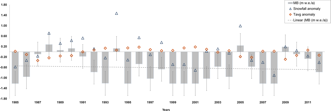
Fig. 4. Modelled annual specific mass-balance estimates of Chandra basin from 1984 to 2012. Bar plot represents area-weighted mean mass balance (m w.e. a−1) for the basin. The uncertainty in model-derived mass balance is shown as vertical lines on the boxes, i.e. ±0.46 m w.e. The grey dashed line is the linear regression line for the mass balance and indicates a mass-balance trend of −0.11 m w.e. a−1 decade−1. Orange diamonds represent normalised (by mean) anomaly in summer temperature, and blue triangles represent normalised anomaly in winter snowfall. It is found that almost all the positive mass-balance years are accompanied by positive anomaly in snowfall and negative anomaly in temperature.
Sensitivity of mass balance to climate variables
We evaluate the sensitivity of mass balance for three cases: ±1 °C change in temperature, ±10 and ±20% change in precipitation. The sensitivity of mass balance to climate variables is calculated following Oerlemans and others (Reference Oerlemans1998). For a 1 °C change in temperature, a change of 85 m in ELA is estimated. This translates to an area-weighted mean sensitivity of 0.16 m w.e. °C−1 in basin-wide mass balance. For individual glaciers, the sensitivity to temperature varies between 0.01 and 0.59 m w.e. °C−1 (Fig. 5). If precipitation is changed by 10 and 20%, then ELA shifts by 47 and 114 m, respectively. In terms of mass balance, a change of 0.09 m w.e. for a 10% change in precipitation is estimated, with a range of 0.01–0.33 m w.e. (10%)−1. This indicates that a +20% change in winter snowfall would offset the effect of a +1 °C change in summer temperature of the basin.
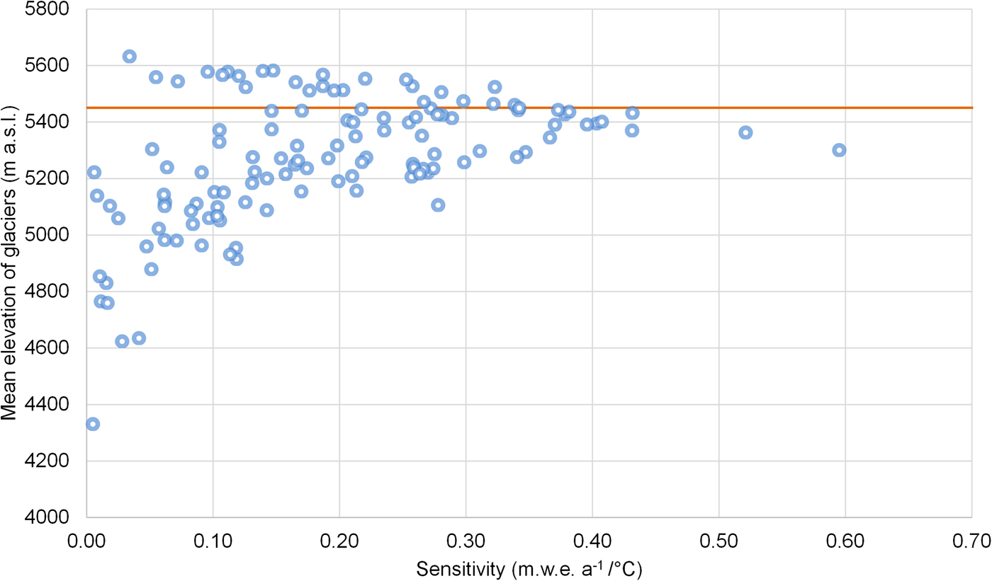
Fig. 5. Sensitivity of mass balance to temperature change versus mean elevation of individual glacier in the basin. The red line indicates the mean ELA of the basin from 1984 to 2012.
We have estimated specific mass balance of individual glaciers, so the altitude-wise mass balance on each glacier is not available. Hence, the altitudinal variations in sensitivity at glacier scale could not be directly estimated. However, we have estimated the mass balance for 146 glaciers with mean altitude ranging from 4175 to 5650 m a.s.l. Therefore, to evaluate the influence of altitude on mass-balance sensitivity, we can use the mean altitude of individual glaciers (Fig. 5). Here we analyse mass-balance sensitivity to temperature, as this is the most commonly discussed quantity in the context of climate change. Sensitivity of mass balance is found to be at a maximum when the mean altitude of the glacier is near the ELA (Fig. 5). This may be because the model-derived mass balance depends on the glacier hypsometry. Therefore, we have grouped glaciers into three categories: top heavy, equidimensional and bottom heavy. The hypsometry index defined by Jiskoot and others (Reference Jiskoot, Curran, Tessler and Shenton2009) is used to classify glaciers based on the area–altitude distributions. We find that 16% of the total glaciers are in the ‘top heavy’ category and they have the highest mass-balance sensitivity of 0.20 m w.e. °C−1. Nearly 34% of the glaciers in the ‘equidimensional’ and 50% in the ‘bottom heavy’ category have mass-balance sensitivities of 0.17 and 0.15 m w.e. °C−1, respectively. The category-wise sensitivity suggests that the ‘bottom heavy’ glaciers are least sensitive, which is in agreement with the results of Jiskoot and others (Reference Jiskoot, Curran, Tessler and Shenton2009).
Volume of the basin
To analyse the proportion of mass loss in the total glacier-stored water, we investigate the glacier volume of the basin. The total surface area of the selected glaciers is 654.29 km2. The total ice volume estimated for these glaciers is 62.10 ± 16 Gt w.e. The ice thickness along the central flowline (h f) of glaciers ranges between 17 ± 4 and 268 ± 56 m. The volume of individual glaciers in the basin varies between 0.06 ± 0.02 and 21.32 ± 6 Gt w.e. (Fig. 6). The uncertainty in the volume is calculated as ±26%. The highest volume is estimated for Bara Shigri Glacier, and only 8% of the total number of glaciers have a volume of >1 Gt w.e. Hypsometric information on the volume indicates that nearly 99% of the total water volume in the basin is located at mean glacier elevations of 4600–5600 m a.s.l (Fig. 7).

Fig. 6. Spatial distribution of water stored in individual glaciers of the Chandra basin. The highest volume is estimated for Bara Shigri (21.32 ± 6 Gt w.e.) and Samudra Tapu Glacier (12.33 ± 3 Gt w.e.). The box represents selected glaciers in low-altitude regions of the basin, where 67% of loss in glacier-stored water is estimated.
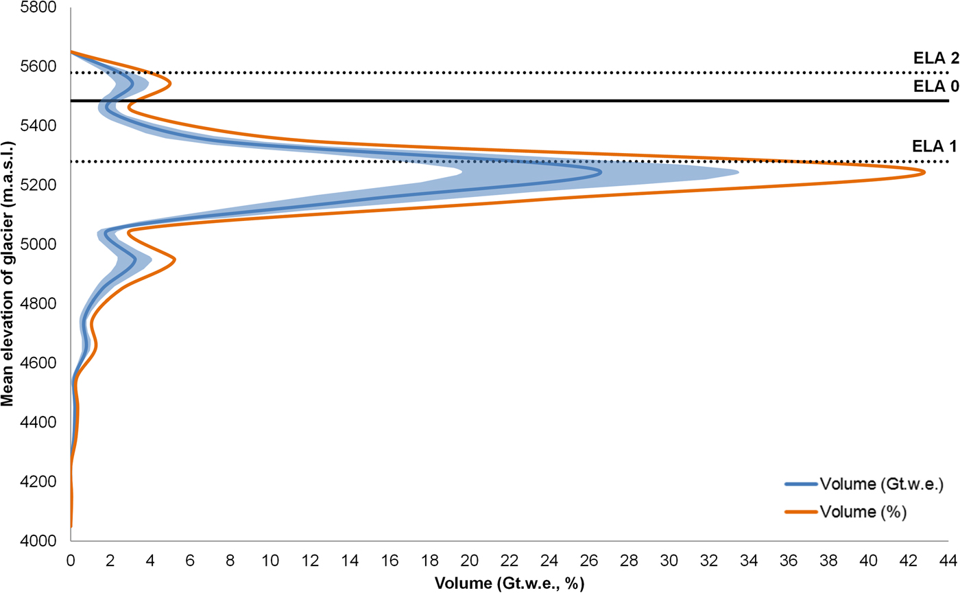
Fig. 7. Hypsometric distribution of volume with respect to the mean glacier elevation in the Chandra basin. Blue line represents volume in Gt w.e., with shaded area as uncertainty. Orange line represents fractional (%) volume stored at each elevation band. ELA0 is the mean ELA of the basin from 1984 to 2012. ELA1 and ELA2 are the mean ELAs of the decades 1985–95 and 1995–2005, respectively.
Cumulative volume loss
Cumulative mass loss of the basin indicates acceleration from the 1990s and especially after 1995 (Fig. 8). In total, the Chandra basin has experienced a water loss of 11.1 ± 8 Gt from 1984 to 2012, which is approximately one-fifth of the total estimated volume. Out of this, the basin has lost 1.17 ± 2 Gt w.e. in the 1980s, 5.03 ± 3 Gt w.e. in 1990s and 4.20 ± 3 Gt w.e. in the 2000s. This sharp reduction in glacier mass from the 1990s can partially be explained by temperature rises of +4 and +2 °C in the 1990s and 2000s, respectively, compared with temperatures in the 1980s.
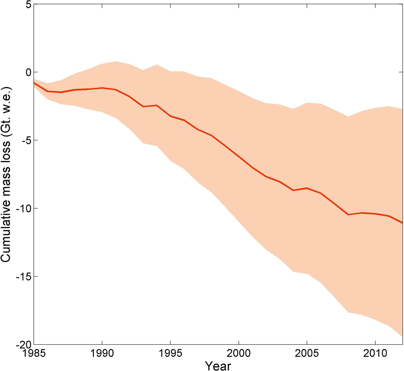
Fig. 8. Cumulative mass balance of the Chandra basin from 1984 to 2012 in Gt w.e. Uncertainty in the model-derived mass balance is shown by the shaded area. Mass loss of the basin is found to have accelerated from the 1990s, especially after 1995. It is found that the basin has lost 11.1 ± 8 Gt of water out of 62.10 ± 16 Gt of the total estimated water volume.
Hypsometry of volume suggests that 94.5% of the total volume of the glaciers is below the mean ELA of the basin (ELA0 in Fig. 7). Between 1985–95 and 1995–2005, the mean summer temperature and winter snowfall of the basin have changed approximately by +2 °C and −20%, respectively. This is equivalent to a rise in ELA by 300 m and a 44% decrease in the ice volume stored above the ELA of the glaciers (Fig. 7).
DISCUSSION
Comparison of mass-balance estimates
In Chandra–Bhaga and surrounding basins, numerous investigations have been carried out to estimate ELA (Kulkarni and others, Reference Kulkarni, Rathore and Alex2004; Pandey and others, Reference Pandey, Kulkarni and Venkataraman2013b, Reference Pandey, Ali, Ramanathan, Champati ray and Venkataraman2016; Guo and others, Reference Guo2014). These investigations are based on field- or satellite-derived snowlines at the end of summer (Kulkarni and others, Reference Kulkarni, Rathore and Alex2004; Pandey and others, Reference Pandey, Kulkarni and Venkataraman2013b; Guo and others, Reference Guo2014; Azam and others, Reference Azam2016). In addition, these investigations are available for different time frames, i.e. 1980–2009. Thus, we find a large variation in ELA (Table 2). For example, in Chandra–Bhaga basin, the mean ELA is estimated at 5009 ± 61 to 5401 ± 21 m a.s.l. for the period 1980–2007 (Pandey and others, Reference Pandey, Kulkarni and Venkataraman2013b). For the adjacent Baspa basin, the ELA varies between 4960 and 5560 m a.s.l. for the years 2000–02 (Kulkarni and others, Reference Kulkarni, Rathore and Alex2004), and for the western Himalaya, it varies between 4840 and 5770 m a.s.l. during 1998–2009 (Guo and others, Reference Guo2014). This is comparable with our mean ELA estimate of 5460 ± 130 m a.s.l. for the period 1984–2012. Though the model-derived ELA of the basin is comparable with snowline altitudes at a larger spatial scale, it is higher than the field-derived ELA of Chhota Shigri Glacier, i.e. 5056 m a.s.l. (Azam and others, Reference Azam2016). This is likely due to the different orientations of glaciers (Kulkarni and others, Reference Kulkarni, Rathore and Alex2004; Guo and others, Reference Guo2014) and the presence of several small glaciers in the basin. Model-derived mean AAR (0.34 ± 0.1) is also consistent with the satellite-derived AAR of 0.44 between 1980 and 2014 for the same basin (Pandey and others, Reference Pandey, Ali, Ramanathan, Champati ray and Venkataraman2016).
Table 2. Comparison of model-derived ELA (m a.s.l.) and AAR and mass-balance (m w.e. a−1) estimates with other studies at basin or larger spatial scales
* The present study covers the period 1984/85 to 2011/12 (here referred as 1984–2012).
† Modelled mass balance is restricted to the Chandra basin.
‡ The height change is converted to mass change using ice density of 850 kg m−3.
In order to validate modelled mass balance at basin scale, we compare it with the geodetic method. The geodetic mass-balance estimates covering the basin are available from 1999 to 2012 (Gardelle and others, Reference Gardelle, Berthier, Arnaud and Kääb2013; Vincent and others, Reference Vincent2013; Vijay and Braun, Reference Vijay and Braun2016). The original investigations were carried out for the entire Lahual–Spiti region in the western Himalaya. Therefore, we have extracted the Chandra basin from the published elevation change data by Gardelle and others (Reference Gardelle, Berthier, Arnaud and Kääb2013) and Vijay and Braun (Reference Vijay and Braun2016). The geodetic mass balance for the basin is −0.68 ± 0.15 and −0.65 ± 0.04 m w.e. a−1 for the periods 1999–2011 and 2000–12, respectively (Table 2). Our mass-balance estimates are −0.66 ± 0.46 m w.e. a−1 for 1999–2011 and −0.63 ± 0.46 m w.e. a−1 for 2000–12. Kääb and others (Reference Kääb, Berthier, Nuth, Gardelle and Arnaud2012) estimate elevation changes in a 2° × 2° cell around Chhota Shigri Glacier using the Ice, Cloud and land Elevation Satellite (ICESat) data and estimate a mass balance of −0.66 ± 0.07 m w.e. a−1 for 2003–08. The Chandra basin occupies 5% of the total area covered in Kääb and others (Reference Kääb, Berthier, Nuth, Gardelle and Arnaud2012), and our mass estimate for the same period is −0.74 ± 0.46 m w.e. a−1.
Mass-balance estimates in earlier studies on global, regional and individual glacier scales overlapping the same period have shown wide variation (Vincent, 2002; Zemp and others, Reference Zemp2008; Braithwaite, Reference Braithwaite2009; Cogley, Reference Cogley2009; Fujita and Nuimura, Reference Fujita and Nuimura2011; Bolch and others, Reference Bolch2012; Huss, Reference Huss2012; Azam and others, Reference Azam2014a). Mass-balance estimates on a global scale are available for the period 1860–2010, and show a sudden drop in glacier mass balance in the 1990s compared with the previous decades (Dyurgerov and Meier, Reference Dyurgerov and Meier2000; Zemp and others, Reference Zemp2008; Braithwaite, Reference Braithwaite2009; Cogley, Reference Cogley2009). For example, Zemp and others (Reference Zemp2008) found that the mass loss rate in 1995–2005 (−0.58 m w.e. a−1) is twice that in 1985–95 (−0.25 m w.e. a−1). Similar results are also observed at regional scales in the European Alps (Vincent, 2002; Huss, Reference Huss2012) as well as over the Himalaya (Fujita and Nuimura, Reference Fujita and Nuimura2011; Bolch and others, Reference Bolch2012). The value reported for the Alps in the 1980s is −0.40 m w.e. a−1 and is −0.84 m w.e. a−1 for 1990–2010 (Huss, Reference Huss2012). Our modelled mass-balance rate for the basin is in close agreement with the analysis of aforementioned studies (Table 2). The warming after 1990 in the Himalayan regions could partly explain the increase in model-derived mass loss (Bhutiyani and others, Reference Bhutiyani, Kale and Pawar2010; Banerjee and Azam, Reference Banerjee and Azam2016).
Our results also partly agree with the model estimates for Chhota Shigri Glacier, where a change in mass balance is observed after 1999. The reported mass balance for the glacier is between −0.018 and +0.09 m w.e. a−1 during 1988–99 (Vincent and others, Reference Vincent2013; Azam and others, Reference Azam2014a) and −0.56 m w.e. a−1 after 1999 (Azam and others, Reference Azam2014a). Our estimates suggest a basin-wide mass loss of −0.57 ± 0.46 and −0.69 ± 0.46 m w.e. a−1 in 1988–99 and 1999–2010, respectively. Our basin-wide results differ from those obtained over Chhota Shigri Glacier for the period 1988–99 because, though the AAR/mass-balance relation is based on field measurements at Chhota Shigri Glacier, the basin-wide modelled mass-balance estimates are also influenced by area–altitude distributions, which vary from glacier to glacier.
Comparison of sensitivity estimates
ELA and mass-balance sensitivity to climate variables at regional scale have been carried out in different parts of the globe, i.e. the Canadian Rockies, Swiss Alps, French Alps, Australian Alps, Norway, Arctic and Himalaya (Oerlemans and Fortuin, Reference Oerlemans and Fortuin1992; Braithwaite and Zhang, Reference Braithwaite and Zhang1999; Braithwaite and others, Reference Braithwaite, Zhang and Raper2002; Vincent, 2002; Oerlemans and others, Reference Oerlemans2005; Woul and Hock, Reference Woul and Hock2005; Zemp and others, Reference Zemp, Hoelzle and Haeberli2007; Rabatel and others, Reference Rabatel, Letréguilly, Dedieu and Eckert2013; Rasmussen, Reference Rasmussen2013; Thibert and others, Reference Thibert, Eckert and Vincent2013; Six and Vincent, Reference Six and Vincent2014; Shea and Immerzeel, Reference Shea and Immerzeel2016). ELA sensitivity reported in the European Alps varies between 50 and 115 m °C−1 (Kuhn, Reference Kuhn and Oerlemans1989; Vincent, 2002; Zemp and others, Reference Zemp, Hoelzle and Haeberli2007; Rabatel and others, Reference Rabatel, Letréguilly, Dedieu and Eckert2013; Thibert and others, Reference Thibert, Eckert and Vincent2013; Six and Vincent, Reference Six and Vincent2014). For Beas basin in the Himalaya, the estimated ELA response to temperature change is large (164 m °C−1, Shea and Immerzeel, Reference Shea and Immerzeel2016). However, this larger sensitivity for Beas basin is estimated by considering annual precipitation (of 1740 mm). According to the function derived by Shea and Immerzeel (Reference Shea and Immerzeel2016), the Chandra basin has a sensitivity of ~73 m °C−1 for the annual precipitation of ~461 mm at the lowest glacier altitude. Our modelled estimate of ELA sensitivity for the basin (85 m °C−1) agrees closely with this value.
The mass-balance sensitivity is reported in a range of 0.1–1.3 m w.e. °C−1 when glaciers around the world are considered (Oerlemans and Fortuin, Reference Oerlemans and Fortuin1992; Braithwaite and Zhang, Reference Braithwaite and Zhang1999; Braithwaite and others, Reference Braithwaite, Zhang and Raper2002). It varies from 0.2 to 2.0 m °C−1 for Arctic glaciers (Woul and Hock, Reference Woul and Hock2005) and between 0.2 and 0.5 m w.e. °C−1 for glaciers in high Asia (Rasmussen, Reference Rasmussen2013). The observed sensitivity to precipitation is in the range 0.03–0.36 m (10%)−1 for Arctic glaciers (Woul and Hock, Reference Woul and Hock2005). The sensitivity reported at glacier scale in the Himalaya is higher, varying from 0.47 to 0.52 m w.e. °C−1 for temperature and from 0.14 to 0.16 m w.e. (10%)−1 (Mölg and others, Reference Mölg, Maussion, Yang and Scherer2012; Azam and others, Reference Azam2014a) for precipitation. Our area-weighted mean sensitivity of the basin is 0.16 m w.e. °C−1 for temperature and 0.09 m w.e. (10%)−1 for precipitation.
From the above discussion, we find that our modelled ELA sensitivity is in agreement with available literature on glacier and regional scales but the mass-balance sensitivity is in agreement only at regional scale. This may be because the model-derived mass balance is controlled by the position of the ELA as well as the area–altitude distribution of individual glaciers. Therefore, for a change in ELA, the response in terms of mass balance will be divergent depending on the area above/below the ELA. This is further discussed in the Results subsection above on sensitivity of mass balance to climate variables.
CONCLUSION
We have analysed annual mass-balance estimates at basin scale using a simple model and limited inputs, in order to fill the gap in mass-balance series over the Himalaya. The present study is a sequel to Tawde and others (Reference Tawde, Kulkarni and Bala2016), where the improved AAR method to estimate mass balance was described using satellite-derived snowlines and the TI model. The method calculates the position of the ELA using temperature and precipitation data. Then the mass balance is derived using AAR/mass-balance regression developed for the basin. The performance of the present approach is dependent on two main quantities: reliable climate data and AAR/mass-balance regression. A detailed discussion on uncertainty in the present approach is provided in Tawde and others (Reference Tawde, Kulkarni and Bala2016).
In the present study, for the first time, we estimate annual mass balance of glaciers in the Chandra basin for almost three decades. We have modelled the annual specific mass balance of 146 glaciers in the basin from 1984 to 2012. Our model results yield a mean ELA of the basin of 5460 ± 130 m a.s.l. The area-weighted mean mass balance is estimated at −0.61 ± 0.46 m w.e. a−1, which is equivalent to 11.1 ± 8 Gt of water loss from the basin in 28 years. The results of the sensitivity analysis show that a 20% increase in winter precipitation can balance the basin-wide mass-balance changes for a 1 °C rise in summer temperature. According to our estimates, the total water volume of the basin is 62.1 ± 16 Gt, which is equivalent to 0.18 mm of mean sea-level rise. Approximately 94% of this is calculated to be in the ablation zone of glaciers. This suggests that future glacier wastage would continue even in the absence of global warming.
Even though, on a basin scale, only 18% of the total glacier-stored water has been lost during 1984–2012, the loss could be large for many small and low-altitude glaciers (Fig. 6). For example, 29 glaciers located in the lower altitudinal range have lost 67% of water. This substantial loss suggests that small villages located in this valley may experience water scarcity.
SUPPLEMENTARY MATERIAL
The supplementary material for this article can be found at https://doi.org/10.1017/aog.2017.18.
ACKNOWLEDGEMENT
We are grateful to the Divecha Centre for Climate Change and Centre for Atmospheric and Oceanic Sciences at the Indian Institute of Science, Bangalore, India, for providing laboratory facilities. We also thank the US Geological Survey for making ASTER GDEM data available. ASTER GDEM is a product of METI and NASA. We acknowledge Etienne Berthier and Saurabh Vijay for providing geodetic estimates for the Chandra basin. We also thank the Bhakra Beas Management Board (BBMB) for meteorological data of Kaza station. Reviews by F. Azam and an anonymous reviewer helped to improve an earlier version of the manuscript.


 Open access